How Does the Built Environment Affect Drunk-Driving Crashes? A Spatial Heterogeneity Analysis

Abstract

In this research, 3356 alcohol-related traffic crashes were obtained from blood-alcohol test reports in Tianjin, China. Population density, intersection density, road density, and alcohol outlet densities, including retail density, entertainment density, restaurant density, company density, hotel density, and residential density, were extracted from 2114 traffic analysis zones (TAZs). After a spatial autocorrelation test, the multiple linear regression model (MLR), geographically weighted Poisson regression model (GWPR), and semi-parametric geographically weighted Poisson regression model (SGWPR) were utilized to explore the spatial effects of the aforementioned variables on drunk-driving crash density. The result shows that the SGWPR model based on the adaptive Gaussian function had the smallest AICc value and the best-fitting accuracy. The residential density and the intersection density are global variables, and the others are local variables that have different influences in different regions. Furthermore, we found that the influence of local variables in the economic–technological development area shows significantly different characteristics compared with other districts. Thus, a comprehensive consideration of spatial heterogeneity would be able to improve the effectiveness of the programs formulated to decrease drunk driving crashes.

1. Introduction

Motor vehicle accidents cause both fatal injury and economic loss to individual households as well as cities all over the world. It is noteworthy that nearly 30% of serious crashes are related to alcohol [1]. In China, 2384 people were killed and 5616 were injured in alcohol-impaired driving crashes in 2014 [2]. Similarly, in Europe, driving under the influence of alcohol (DUI) was linked to around 25% of road deaths [3]. The severe consequences have driven efforts from many aspects to prevent drunk driving.

The primary objective of this study is to explore the spatial heterogeneity of the correlation between the built environment factors related to drunk-driving crashes and the risks of drunk-driving crashes by a case study. More specifically, this paper aims to answer the following research questions: (a) whether the spatial heterogeneity model is more suitable to describe the aforementioned spatial correlation than the traditional global regression models; (b) which spatial heterogeneity model is more suitable to describe this correlation; (c) which factors are global variables and which of them are local variables; (d) what are the distribution characteristics of the regression coefficients for the local variables in the urban area? In addition, we hope that the expected findings could contribute to predicting drunk-driving crashes more accurately and guide the planners to improve traffic safety planning.

The remainder of the paper is organized as follows. Section 2 mainly introduces the research status of related factors in drunk-driving crashes and the spatial models for traffic crash analysis. Section 3 describes the data sources, preprocessing, and methodology of this research, including the multiple linear regression (MLR) model, geographically weighted Poisson regression (GWPR) model, and semi-parametric geographically weighted Poisson regression (SGWPR) model. Section 4 shows the results of different models followed by the analysis. Section 5 compares the results and discusses the spatial heterogeneity of the explanatory variables. Finally, Section 6 concludes the major findings and the potential implications of this research.

2. Literature Review

Previous research has proven that the factors leading to traffic crashes can be divided into several groups, which are traffic participants, vehicles, roads, and the environment [4]. Unlike common traffic accidents, the main cause of drunk-driving crashes is that the driver drinks alcohol before driving, which leads to degradation in driving performance. Thus, a ratiocination can be gained that drunk drivers and alcohol availability-related factors, e.g., the alcohol outlet densities, are correlated with the local risk of traffic accidents [5].

2.1. The Influence of Drunk Driving Drivers

In order to support the refined management of drunk driving, researchers continuously explored the key factors which may lead to alcohol-related crashes. A few researchers summarized the regular patterns of drunk driving behaviors based on drivers’ specific attributes like age and gender and further evaluated drunk driving risks by different groups, e.g., older adults [6], adolescents [7], middle-aged, and mature-aged women [8]. Moreover, some studies showed that the distinctive alcohol consumption culture and patterns in different areas would result in the different local risks of drunk-driving crashes, e.g., United States [9], India [10], Cambodia [11], Spain [12], and France [13].

2.2. The Influence of Alcohol Outlets on Drunk Driving Crashes

Naturally, there has been increasing research attention paid to the relationships between alcohol outlet density and drunk driving crashes. Alcohol outlets generally refer to the sources where alcohol is sold or consumed, such as homes, retail stores, liquor stores, bars, restaurants, entertainment venues, hotels, and drive-up liquor windows [14]. Gruenewald et al. concluded that alcohol availability is significantly related to rates of single vehicle night-time crashes (SVNs) [15]. They also determined the positive correlation between restaurant density and SVNs as well as the negative correlation between bar density and SVNs. Curtis et al. found that the rates of drunk driving are very likely to be related to the density of bars [16]. In addition, 74% of drunk drivers were arrested at an average distance of 3.4 miles from the drinking place in New Mexico, and 17.3% of respondents expressed that alcohol consumption happened during meals, according to a case study in Spanish [17]. Furthermore, some studies found that there was a negative correlation between off-premise outlets and crashes, while a positive correlation exists between on-premise outlets and crashes [18]. Meanwhile, other research based on different case studies argued that the densities of off-premise establishments and local bars were positively correlated with the local alcohol-related crash rates [5]. After the close relationship between traffic crashes and the built environment factors associated with alcohol availability eventually demonstrated by numerous studies, more attention has been paid to spatial analysis in recent years [19].

2.3. Spatial Analysis for Traffic Crashes

Commonly used crash models in the existing studies include ordinary least squares regression models [20], Poisson and Poisson-extended models [21], negative binomial regression models [22], zero-inflated models [23], hurdle models [24], logistic regression models [1], Bayesian models [25], and the conditional autoregressive prior (CAR) model [26]. However, the above-mentioned studies assume that the influence of explanatory variables on the explained variable does not change with the spatial position, which means that the models used for analysis do not take spatial heterogeneity into consideration [19].

Tobler’s first law of geography laid the foundation of spatial analysis for traffic crashes. It indicates that the more adjacent things are, the more related they are to each other. Since the approaches of spatial analysis were introduced to the field of traffic safety, researchers kept working on uncovering the spatial autocorrelation and heterogeneity of traffic crashes and related variables. In this regard, the spatial lag model, spatial error model, and spatial Durbin model were applied to explore the spatial autocorrelation between residential and demographic factors as explanatory variables and the traffic crashes as the explained variable based on different spatial scales, including states, countries, segments, regions, traffic analysis zones (TAZ), zip codes, and census tracts [4]. However, compared with spatial autocorrelation, the spatial heterogeneity of alcohol-related crashes is rarely studied, whereas for megacities with complex and diverse build environments, spatial heterogeneity should not be excluded. Greene et al. proved that the social context, rural cultural values, and the legal and physical environment promote the frequency of drunk driving more significantly in rural areas rather than in the downtown [27]. Similarly, by analyzing breath-testing data, Armstrong et al. found that the detection rate in rural areas was higher than that in urban areas [28].

Regarding this matter, the geographically weighted regression (GWR) model has been employed to analyze traffic crashes to recognize the spatial heterogeneity of different explanatory variables. Bao et al. used the GWR model to examine the relationships between crash counts and various contributing factors based on Twitter-based human activity information data [29]. Huang et al. proposed a GWR model and revealed the spatially non-stationary between the built environment and traffic crashes [19]. Nevertheless, to our knowledge, little research has been conducted on the spatial heterogeneity of the built environment factors to the drunk driving crashes. This manuscript provides Chinese case studies for researchers from other countries and regions around the world.

3. Methods

Aiming at exploring the spatial heterogeneity of build environment factors on the drunk driving crashes, this study followed a three-step analysis framework. Firstly, a multiple regression model was used to explore the linear correlation between drunk-driving crashes and related influence factors without spatial heterogeneity. Secondly, the optimal GWR model was established to calculate the regression coefficients varying over space based on different bandwidth and spatial weight functions. Thirdly, the MGWR model was formulated to distinguish the global variables and local variables.

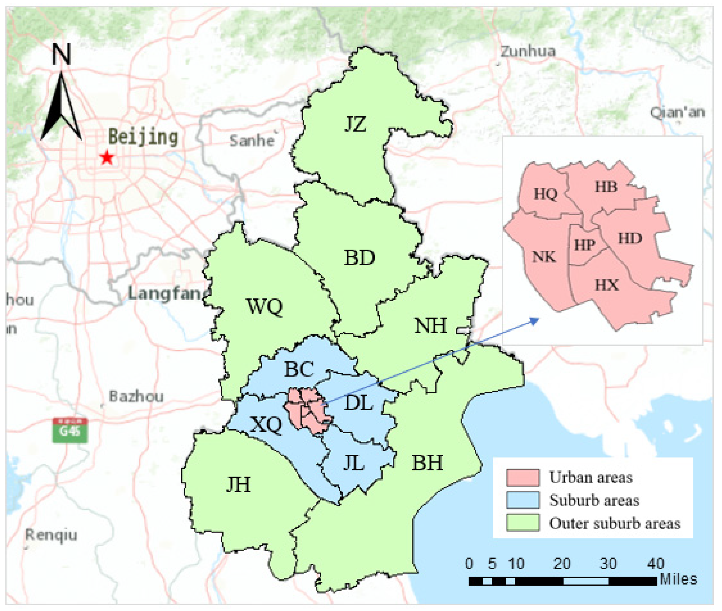
3.1. Data Preparation

Drivers with a blood-alcohol content of more than or equal to 0.02 g/dL are considered drunk drivers under the law of road traffic safety in China. In total, 3356 cases of drunk-driving crashes were obtained by extracting the driver’s blood-alcohol test report from 2011 to 2013 in Tianjin, China, a Chinese megacity with area of 11,966.45 square kilometers and a population of over 15.61 million. As shown in Figure 1, the whole city consists of 16 districts, which are divided into 2214 TAZs based on land use attributes, and 54.6% of TAZs have zero alcohol crashes. Built environment variables like population density, intersection density, and road density were extracted from the Transportation Planning and Design Institute of Tianjin. In addition, the points of interest (POI) data closely related to the source of alcohol were extracted based on a web crawler, based on the variables representing alcohol availability, including retail density, entertainment density, restaurant density, company density, hotel density, and residential density were generated [30]. All the explanatory variables were aggregated into TAZs, which were defined as the analysis unit in this research.

In order to narrow the range of the variables and avoid the model being over-sensitive to extreme values, a logarithm was taken for all variables. Meanwhile, the existence of multicollinearity between the explanatory variables may lead to the estimation deviation; thus, the variance inflation factor (VIF) was calculated to test the multicollinearity problems. As shown in

Table 1. Descriptive statistical table of variables.

Category	Variables	Definition	Mean	Minimum	Maximum	VIF
Explained variable	Crash_den	Number of alcohol-related crashes per square kilometer	0.36	0.00	4.41	-
Explanatory variables	Pop_den	People per square kilometer	7.02	−0.69	11.42	1.89
	Retail_den	Number of retail stores per square kilometer	1.35	−5.00	8.10	7.29
	Entertainment_den	Number of entertainment places per square kilometer	0.78	−4.85	5.82	6.56
	Restaurant_den	Number of restaurants per square kilometer	0.97	−4.88	6.89	8.72
	Company_den	Number of companies per square kilometer	1.68	−3.36	5.15	2.40
	Hotel_den	Number of hotels per square kilometer	0.22	−4.64	4.14	2.04
	Residential_den	Number of residences per square kilometer	0.78	−4.85	5.16	3.97
	Intersection_den	Number of Intersection per square kilometer	1.34	−4.33	4.64	4.50
	Road_den	Length of road per square kilometer	0.81	−6.75	3.10	3.70

, no variables with the VIF more than 10 could be found, which indicated all the explanatory variables passed the VIF test and could be reserved in the model.

3.2. Spatial Correlation Test

Moran’s I is widely used to measure the spatial autocorrelation of the variables [31]. The result indicates whether the spatial distribution of the variable is autocorrelation or random [32]. Thus, we calculated Moran’s I under the “rook” spatial weight matrix as Equation (1) to determine whether the null hypothesis could be rejected for the variables selected in this research.

$$Mora{n}^{\prime }s I=\frac{N}{{\sum }_i{\sum }_j{c}_{ij}}\frac{{\sum }_i{\sum }_j{c}_{ij}\left(E_i-\overline{E}\right)\left(E_j-\overline{E}\right)}{{\sum }_i\left(E_i-\overline{E}\right)},$$

(1)

where N is the number of TAZs; Ei and Ej represent the proportion of the variables in ith and jth TAZ; E denotes the average proportion of variables across different TAZs; c_ij is the element of the spatial weight matrix (rook in the present study). c_ij equals 1 if TAZ i and j have a common boundary, and 0 otherwise.

3.3. Multiple Linear Regression Model

The MLR model is widely used to estimate the model parameters in traffic safety research [33]. The traditional MLR model is a global model that assumes the correlations between the explained variable and explanatory variables are the same for the whole study area [34]. The model can be expressed as shown in Equation (2). The F-test of the regression equation can verify whether the MLR model has statistical significance, while the t-test of the regression coefficient determines whether the explanatory variables should be reserved in the model [20]. As to the regression results, the larger the adjusted R² is, the better the model can explain the correlation.

$$y_i={\beta }_0+{\sum }_{k=1}^P{\beta }_k{x}_{ik}+{\epsilon }_i,$$

(2)

where y_i stands for the drunk driving crashes density for TAZ i (i = 1, 2, …, 2114), β₀ is the regression constant, P is the number of explanatory variables, β_k (k = 1, 2, …, P) is the regression coefficient of the explanatory variable x_i, and ε_i is the random disturbance terms of independent and identical distribution.

3.4. Geographically Weighted Poisson Regression Model

Obviously, the MLR model cannot estimate the spatial heterogeneity of the correlation between explanatory variables and the explained variable. Thus, the GWPR model that allows the coefficients to vary over space was introduced to extend the MLR model. The GWPR model can be expressed as shown in Equation (3) [35]. The geographic spatial location, e.g., latitude and longitude, of the variables were embedded into the linear model, and therefore the spatial heterogeneity could be analyzed.

$$\begin{gathered} y_i\sim Poisson\left({\lambda }_i\right), \\ \mathit{ln}({\lambda }_i)={\beta }_0(u_i,v_i)+{\sum }_{k=1}^P{\beta }_k\left(u_i,v_i\right)x_{ik}+{\epsilon }_i, \end{gathered}$$

(3)

where λ_i is the parameter of the Poisson model (i.e., the expected number of crashes in TAZ i), (u_i, v_i) stands for the coordinate of the TAZ i (i = 1, 2, …, 2114), and β_k (u_i, v_i) represents the regression coefficient k of the TAZ _i.

3.5. Semi-Parametric Geographically Weighted Poisson Regression Model

Not all the correlations of regression parameters in the GWPR model vary over space. For some parameters, they are fixed, or the spatial heterogeneities are exceedingly small and can be ignored. The explanatory variables with geographically varying coefficients are called local variables, while the variables with coefficients that do not change with spatial location are called global variables. SGWPR considers the spatial effects for both global variables and local variables, which can be conducive to exploring the spatial heterogeneity of the factors related to drunk driving crashes. The framework of SGWPR is as follows [36]:

$$\begin{gathered} P_a+P_b=P, \\ \mathit{ln}({\lambda }_i)={\beta }_0\left(u_i,v_i\right)+{\sum }_{j=1}^{P_a}{\beta }_j{x}_{ij}+{\sum }_{k=1}^{P_b}{\beta }_k\left(u_i,v_i\right)x_{ik}+{\epsilon }_i, \end{gathered}$$

(4)

where Pa is the number of the global variables, β_j denotes the coefficient of the global variables j, P_b is the number of the local variables, and β_k represents the coefficient of the local variables k.

The result of the GWPR model is sensitive to the spatial kernel function and bandwidth size. In most research, the adaptive kernel function is more effective compared with the fixed kernel function because it permits the bandwidth to vary spatially [34]. However, the effect of kernel function and bandwidth is not clear for drunk-driving crashes and the related factors. Therefore, the spatial regression models with fixed bandwidth and adaptive bandwidth, as well as both types of commonly used kernel functions, including the Gaussian kernel function and the bi-square kernel function, as shown in Equation (5), were comprehensively tested in this research. The corrected Akaike information criterion (AICc) was used to compare the results and select the best spatial model [37].

$$\begin{gathered} \mathrm{Gaussian}: W_{ij}=e^{-{\left(\frac{d_{ij}}{b}\right)}^2}, \\ \mathrm{bi}-\mathrm{square}: W_{ij}={\left\{\begin{array}{c}\left[1-{\left(\frac{d_{ij}}{b_i}\right)}^2\right]\\ 0, d_{ij}>b_i\end{array}\right.}^2, d_{ij}\le b_i, \end{gathered}$$

(5)

where W_ij is the spatial weight function to describe the influence of TAZ j on TAZ i, d_ij is the European distance between TAZ i and TAZ j, b is the fixed bandwidth defined by the distance in the Gaussian function, and b_i is adaptive bandwidth defined as the number of the adjacent TAZs around the target TAZ.

In the GWPR model, the local percent deviance explained pdev instead of local R² are calculated to estimate the local goodness-of-fitness, which indicates how well the model fits the data. The local pdev is defined as follows:

$${pdev}_i=1-\frac{{dev}_i}{{nulldev}_i},$$

(6)

where dev_i is the locally weighted deviance of the fitted model, and nulldev_i is the locally weighted deviance of the null model having only a constant term at location i.

4. Results

4.1. Results of Moran’s I

Table 2. Moran’s I test results.

Variables	Moran’s I	Pattern	Z-Score	p-Value
Crash_den	0.331	Clustered	22.807	0.001
Pop_den	0.752	Clustered	51.732	0.001
Retail_den	0.718	Clustered	61.454	0.001
Entertainment_den	0.702	Clustered	48.280	0.001
Restaurant_den	0.722	Clustered	49.638	0.001
Company_den	0.880	Clustered	60.558	0.001
Hotel_den	0.487	Clustered	33.529	0.001
Residential_den	0.728	Clustered	50.105	0.001
Intersection_den	0.656	Clustered	45.090	0.001
Road_den	0.574	Clustered	39.512	0.001

shows the results of Moran’s I. The Z-scores of all the variables were positive and statistically significant at a 1% level, which indicated that the spatial distribution of both explained variables and explanatory variables are clustered. Therefore, the selected variables satisfied the prerequisite for analysis by the GWPR model.

4.2. Results of the MLR Model

The linear correlation between drunk-driving crashes and related influencing factors without spatial effect was first analyzed based on the MLR model. The adjusted R² of the model was 0.316, and the p-value of the F-test was less than 0.001, which indicated the statistical significance of the result. In total, the MLR model could explain 31.6% of the occurrence of drunk-driving crashes. As shown in

Table 3. Coefficient estimation of MLR model.

Variables	Coefficients	t-Statistic	p-Value
Pop_den	0.193	7.779	0.001
Retail_den	0.483	9.918	0.001
Entertainment_den	−0.018	−0.381	0.704
Restaurant_den	0.006	0.110	0.913
Company_den	−0.680	−24.348	0.001
Hotel_den	−0.108	−4.190	0.001
Residential_den	−0.105	−2.911	0.004
Intersection_den	0.074	1.927	0.048
Road_den	0.103	2.959	0.003

, the population density, retail density, restaurant density, intersection density, and road density were positively correlated with crash alcohol-related density, while the correlations between entertainment density, company density, hotel density, residential density, and crash density were negative. Similar to previous studies, the results of the t-test for entertainment density and restaurant density were not significant [3]. Moreover, the t-test of intersection density was significant at a 5% level, and the other explanatory variables were significant at a 1% level. Therefore, the entire variables except entertainment density and restaurant density were used to further estimate the effect of spatial heterogeneity.

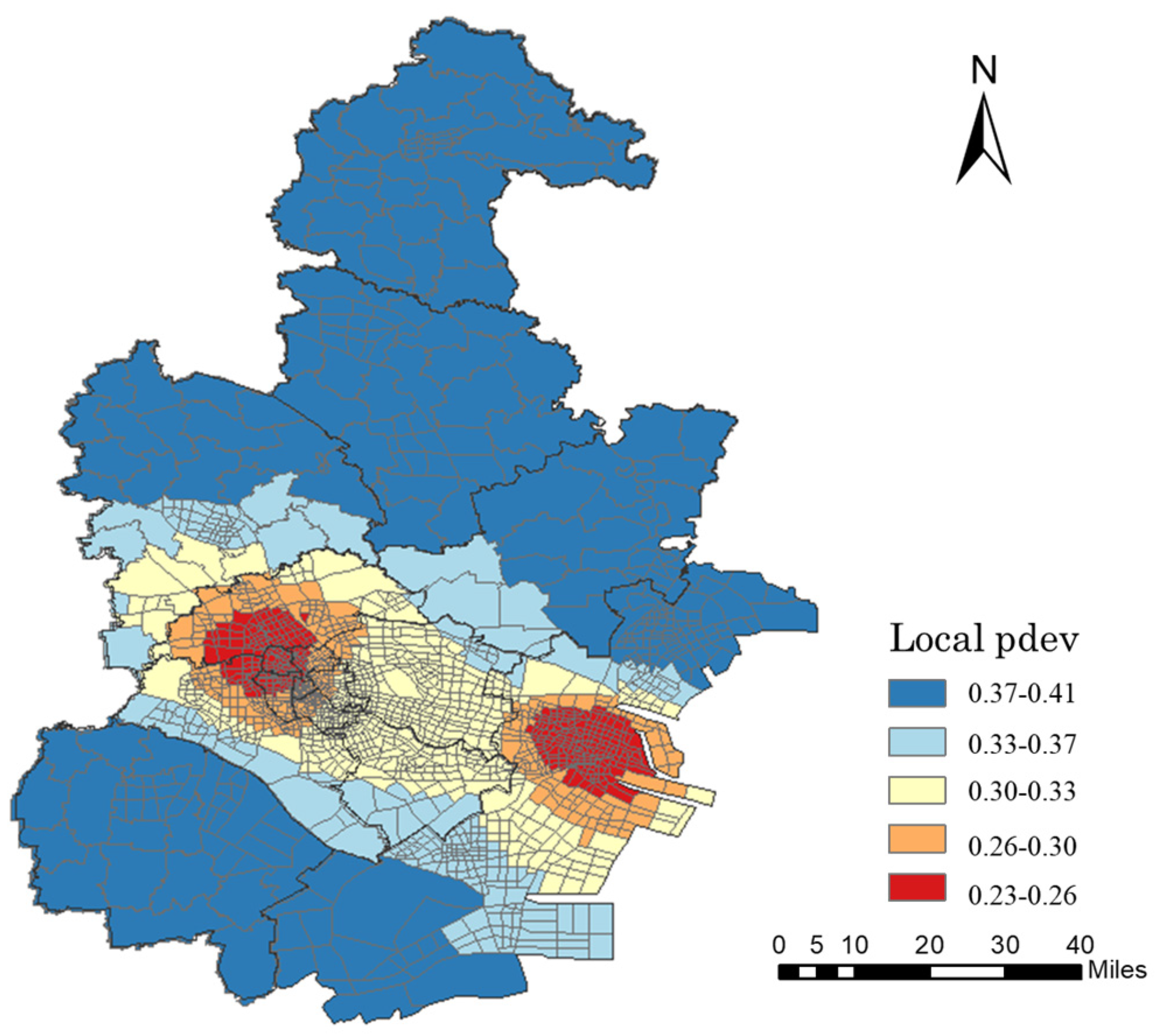
4.3. Results of the GWPR Model

As shown in

Table 4. Fitting results of GWPR model.

Model	MLR	GWPR		GWPR		SGWPR
Kernel Functions	-	Adaptive Bi-Square	Adaptive Gaussian	Adaptive Bi-Square	Adaptive Gaussian	Adaptive Bi-Square	Adaptive Gaussian
Best bandwidth size	-	1386	215	1172	147	303.14	237.62
AICc	1385.20	1355.79	1350.56	1348.00	1339.52	1312.80	1307.91
Number of variables	9	9	9	7	7	7	7
Global Variables	All variables	-		-		Other Explanatory variables	Residential_den Intersection_den
Local Variables		All Explanatory variables		All Explanatory variables except Entertainment_den and Restaurant_den		Company_den	Other Explanatory variables

, different spatial GWPR models were constructed based on the spatial kernel functions of the adaptive bi-square and adaptive Gaussian models. The AICc values in GWPR models were all smaller than those in the MLR model, which indicated that the crash models considering spatial heterogeneity had better fitting accuracy. Moreover, the AICc value of GWPR models dropped after removing the entertainment density and restaurant density. Among the GWPR models, the SGWPR model based on the adaptive Gaussian function had the smallest AICc value and the best fitting accuracy. The best bandwidth of the SGWPR model was 237.62. The global variables of the model were residential density and intersection density, and the local variables were population density, retail density, company density, hotel density, residential density, intersection density, and road density.

Table 5. Descriptive statistic for regression coefficients of local variables in SGWPR model.

Variable	Mean	Min	Max	Robust STD
Intercept	−1.549	−2.225	−1.073	0.256
Population_den	0.397	−0.048	0.606	0.099
Retail_den	0.516	0.129	0.894	0.141
Hotel_den	0.027	−0.190	0.576	0.060
Company_den	−1.421	−1.809	−0.677	0.222
Road_den	0.109	−0.080	0.308	0.128

lists the descriptive statistics of the regression coefficient of the local variables. The regression coefficients of population density, hotel density, and road density were positive in some areas but negative in other areas, indicating significant spatial heterogeneity. Retail density had a positive effect, while company density had a negative effect for all the TAZs. By comparing the standard deviations, it could be found that the value of company density had the most dispersed regression coefficient, which indicated that the difference in influence from company density in different regions was more significant than other variables.

Table 6. Descriptive Statistics for regression coefficient of global variables in SGPWR model.

Variable	Estimate	Standard Error	z(Estimate/SE)
Residential_den	0.094	3.036	0.031
Intersection_den	0.415	3.472	0.120

shows descriptive statistics for the regression coefficient of the global variables. The residential density and intersection density were positively correlated with the drunk driving crashes. The results were consistent with existing literature [13].

As shown in Figure 2, the local pdev values were all greater than 0.23. The spatial distribution of the local pdev indicated that the SGWPR model fitted to the data. It is noteworthy that the size and spatial distribution of the local pdev value in the urban area and the core area of the BH district were basically the same. A major reason for this phenomenon might be that the BH district is not an ordinary outer suburb area but an economic and technological development zone. Meanwhile, the local pdev value of the outer suburb area was especially high, which showed that the SGWPR model fitted the outer suburb area better than urban and suburban areas.

As shown in Figure 3, the spatial distribution of local variables revealed an obvious pattern of spatial heterogeneity. The population density was the “global” positive in the MLR model, while the regression coefficient fluctuated from negative to positive (−0.05 to 0.61) in the SGWPR model. All the coefficients of retail density in different TAZs were positive (0.13 to 0.89), indicating that the increase in retail density always increased the risk of drunk driving crashes. On the contrary, all the coefficients of company density were negative, indicating the common negative correlations between company density and crash density in all TAZs. Moreover, the hotel density was negatively correlated with the crash density in most TAZs but only positively correlated with crash density in very few TAZs along the east and west administrative city boundary. In addition, the coefficients of road density were positive in 80.37% of TAZs, but there were also some TAZs with negative correlations between road density and crash density clustered in the middle-west areas. Generally, the spatial distribution of the value for road density coefficients presented a pattern that decreased approximately from north to south.

5. Discussion

5.1. The Spatial Heterogeneity Characteristics of Variables

The results of this research substantiate that spatial heterogeneity exists in correlations between the density of drunk driving crashes and the related build environment factors. Meanwhile, the spatial heterogeneity shows different patterns for the correlations of different factors. The results of Moran’s I show that the spatial distribution of both explanatory variables and the explained variable are clustered. Compared with the MLR model and GWPR model, the SGWPR model with adaptive Gaussian kernel function and a bandwidth of 237.62 was proved to be the most suitable model to describe the effect of the factors on drunk-driving crashes. The residential density and intersection density are global variables and are positively correlated with the drunk driving crash density. Meanwhile, population density, retail density, hotel density, company density, and road density are local variables, and their correlations with alcohol-related crashes vary over space.

Moreover, an interesting finding is that the influence of local variables in the core area of the BH district shows different characteristics from those in other districts. The correlation between population density and drunk-driving crash density is negative in the core area of the BH district but positive in other districts. The retail density of the TAZs in other districts have a greater positive effect on the risk of drunk-driving crashes than those in the core area of the BH district. It is noteworthy that the distribution of spatial heterogeneity for hotel density and retail density is completely opposite. The reason for this phenomenon may be that the core area of the BH district has frequent traffic activities and business exchanges; people from other places in the BH district usually lodge their accommodation and banquet in hotels, which results in a more significant positive correlation of hotel density to the density of alcohol-involved crashes. The city center of Tianjin and the core area of the Binhai district are all concentration areas of companies. However, the company density of the TAZs in the city core negatively affects the crash density more significantly than that of the TAZs in the Binhai District. The spatial heterogeneity of company density indicates that the startups mainly located in the Binhai District may manage the employees in a different way compared with the large-sized companies in the city core, and the managers should also consider controlling the risk of DUI for employees by adjusting the management mechanism.

5.2. Policy Implications

Based on the results above, we suggest that the traffic police enforce the management of DUI from a new perspective. In common sense, local police assume that drunk-driving crashes are more likely to happen in areas with more people and restaurants. According to the result of this research, the occurrence of drunk-driving crashes is a joint result of global variables and local variables. Therefore, switching more attention to the local variables may help the police to arrange the force more properly. For instance, the police may implement different strategies for deploying checkpoints in various districts according to spatial heterogeneity.

We expect the results of this study could be helpful for the related traffic departments to take measures for eliminating drunk driving behaviors and reducing the occurrence of drunk-driving crashes. Firstly, the quantitative analysis of spatial heterogeneity may help policymakers to formulate different traffic safety countermeasures for different regions, which could improve management efficiency. Secondly, the correlations with spatial heterogeneity could be a reference for urban planners to integrate traffic safety planning into the planning framework of urban infrastructure and road networks, in which way a more precise and refined urban planning could be achieved. Thirdly, online hailing car companies, as well as the companies providing alternative driving services, could optimize their algorithm to gain larger commercial benefits and make efforts to reduce the occurrence of drunk driving crashes based on the results of this study.

5.3. Limitations and Future Directions

The major limitations of this study are as follows. First, the characteristics of the driver should not be ignored. Driving after drinking alcohol is a direct influencing factor that leads to drunk-driving crashes. Thus, demographic characteristics such as age, gender, race, and place of birth, as well as socioeconomic characteristics such as marriage, education, occupation, and income, even including norms and culture, should be used as the characteristics of the population “the drivers”. Second, the variables of alcohol availability are denoted by the density of POIs. Taking the company as an example, the building area, company type, and number of employees are not considered in this study, which may affect the accuracy of the result. Third, the temporal factor should also be integrated to establish the spatiotemporal weighted model for the accurate prediction of drunk-driving crash risk in the future.

6. Conclusions

This study takes the Chinese megacity Tianjin as the case study and utilized MLR, GWPR, and SGWPR models to explore the spatial heterogeneity of the correlations between the build environment factors and drunk-driving crashes. The SGWPR model with adaptive Gaussian kernel function explains the correlations with the spatial heterogeneity best among the selected models. The density of residential and intersections are global variables and have a positive effect on the increase of crashes in all TAZs. On the other hand, population density, retail density, hotel density, company density, and road density are local variables, and their correlations with crash density vary over space. The results prove that spatial heterogeneity is significant for the explanatory variables and cannot be neglected while analyzing the risk of drunk-driving crashes.

References

1. Stephens, A.N.; Bishop, C.A.; Liu, S.; Fitzharris, M. Alcohol Consumption Patterns and Attitudes toward Drink-Drive Behaviours and Road Safety Enforcement Strategies. Accid. Anal. Prev. 2017, 98, 241–251. [Google Scholar] [CrossRef] [PubMed]
2. Wang, S.; Chen, Y.; Huang, J.; Liu, Z.; Li, J.; Ma, J. Spatial Relationships between Alcohol Outlet Densities and Drunk Driving Crashes: An Empirical Study of Tianjin in China. J. Safety Res. 2020, 74, 17–25. [Google Scholar] [CrossRef]
3. Navas, J.F.; Martín-pérez, C.; Petrova, D.; Verdejo-garcía, A.; Cano, M.; Sagripanti-mazuquín, O.; Perandrés-gómez, A.; López-martín, Á.; Cordovilla-guardia, S.; Megías, A.; et al. Sex Differences in the Association between Impulsivity and Driving under the Influence of Alcohol in Young Adults: The Specific Role of Sensation Seeking. Accid. Anal. Prev. 2019, 124, 174–179. [Google Scholar] [CrossRef]
4. Wang, S.; Chen, Y.; Huang, J.; Chen, N.; Lu, Y. Macrolevel Traffic Crash Analysis: A Spatial Econometric Model Approach. Math. Probl. Eng. 2019, 2019, 5306247. [Google Scholar] [CrossRef]
5. Treno, A.J.; Johnson, F.W.; Remer, L.G.; Gruenewald, P.J. The Impact of Outlet Densities on Alcohol-Related Crashes: A Spatial Panel Approach. Accid. Anal. Prev. 2007, 39, 894–901. [Google Scholar] [CrossRef]
6. Kuerbis, A.; Sacco, P. The Impact of Retirement on the Drinking Patterns of Older Adults: A Review. Addict. Behav. 2012, 37, 587–595. [Google Scholar] [CrossRef] [PubMed]
7. Robbins, C.J.; Russell, S.; Chapman, P. Student Drivers the Morning after Drinking: A Willingness to Violate Road Rules despite Typical Visual Attention. Transp. Res. Part F Traffic Psychol. Behav. 2019, 62, 376–389. [Google Scholar] [CrossRef]
8. Armstrong, K.A.; Davey, J.D.; Freeman, J.E.; Young, S.J. A Qualitative Exploration of Apprehended Women’s Experience of Drink Driving Events. Transp. Res. Part F Psychol. Behav. 2020, 69, 49–60. [Google Scholar] [CrossRef]
9. Portman, M.; Penttilä, A.; Haukka, J.; Rajalin, S.; Eriksson, C.J.P.; Gunnar, T.; Koskimaa, H.; Kuoppasalmi, K. Profile of a Drunk Driver and Risk Factors for Drunk Driving. Findings in Roadside Testing in the Province of Uusimaa in Finland 1990–2008. Forensic Sci. Int. 2013, 231, 20–27. [Google Scholar] [CrossRef] [PubMed]
10. Kizhakke Veetil, D.; Ismail, D.M.; Roy, N.; Khajanchi, M.U. Drink-Driving: India Slow on Enforcement. Injury 2016, 47, 508–509. [Google Scholar] [CrossRef]
11. Bachani, A.M.; Risko, C.B.; Gnim, C.; Coelho, S.; Hyder, A.A. Knowledge, Attitudes, and Practices around Drinking and Driving in Cambodia: 2010–2012. Public Health 2017, 144, S32–S38. [Google Scholar] [CrossRef]
12. Alcañiz, M.; Santolino, M.; Ramon, L. Drinking Patterns and Drunk-Driving Behaviour in Catalonia, Spain: A Comparative Study. Transp. Res. Part F Traffic Psychol. Behav. 2016, 42, 522–531. [Google Scholar] [CrossRef]
13. Assailly, J.P.; Cestac, J. Alcohol Interlocks and Prevention of Drunk-Driving Recidivism. Rev. Eur. Psychol. Appl. 2014, 64, 141–149. [Google Scholar] [CrossRef]
14. Lee, J.A.; Jones-Webb, R.J.; Short, B.J.; Wagenaar, A.C. Drinking Location and Risk of Alcohol-Impaired Driving among High School Seniors. Addict. Behav. 1997, 22, 387–393. [Google Scholar] [CrossRef]
15. Gruenewald, P.J.; Millar, A.B.; Treno, A.J.; Yang, Z.; Ponicki, W.R.; Roeper, P. The Geography of Availability and Driving after Drinking. Addiction 1996, 91, 967–983. [Google Scholar] [CrossRef]
16. Curtis, A.; Coomber, K.; Hyder, S.; Droste, N.; Pennay, A.; Jenkinson, R.; Mayshak, R.; Miller, P.G. Prevalence and Correlates of Drink Driving within Patrons of Australian Night-Time Entertainment Precincts. Accid. Anal. Prev. 2016, 95, 187–191. [Google Scholar] [CrossRef] [PubMed]
17. Alonso, F.; Pastor, J.C.; Montoro, L.; Esteban, C. Driving under the Influence of Alcohol: Frequency, Reasons, Perceived Risk and Punishment. Subst. Abuse Treat. Prev. Policy 2015, 10, 11. [Google Scholar] [CrossRef]
18. Campbell, C.A.; Hahn, R.A.; Elder, R.; Brewer, R.; Chattopadhyay, S.; Fielding, J.; Naimi, T.S.; Toomey, T.; Lawrence, B.; Middleton, J.C. The Effectiveness of Limiting Alcohol Outlet Density as a Means of Reducing Excessive Alcohol Consumption and Alcohol-Related Harms. Am. J. Prev. Med. 2009, 37, 556–569. [Google Scholar] [CrossRef]
19. Huang, Y.; Wang, X.; Patton, D. Examining Spatial Relationships between Crashes and the Built Environment: A Geographically Weighted Regression Approach. J. Transp. Geogr. 2018, 69, 221–233. [Google Scholar] [CrossRef]
20. Niederdeppe, J.; Avery, R.; Miller, E.N. Alcohol-Control Public Service Announcements (PSAs) and Drunk-Driving Fatal Accidents in the United States, 1996–2010. Prev. Med. 2017, 99, 320–325. [Google Scholar] [CrossRef]
21. Hosseinpour, M.; Sahebi, S.; Hasanah, Z.; Shukri, A. Predicting Crash Frequency for Multi-Vehicle Collision Types Using Multivariate Poisson-Lognormal Spatial Model: A Comparative Analysis. Accid. Anal. Prev. 2018, 118, 277–288. [Google Scholar] [CrossRef]
22. Zeng, Q.; Huang, H.; Pei, X.; Wong, S.C.; Gao, M. Rule Extraction from an Optimized Neural Network for Traffic Crash Frequency Modeling. Accid. Anal. Prev. 2016, 97, 87–95. [Google Scholar] [CrossRef]
23. Huang, H.; Chin, H.C. Modeling Road Traffic Crashes with Zero-Inflation and Site-Specific Random Effects. Stat. Methods Appl. 2010, 19, 445–462. [Google Scholar] [CrossRef]
24. Cai, Q.; Lee, J.; Eluru, N.; Abdel-Aty, M. Macro-Level Pedestrian and Bicycle Crash Analysis: Incorporating Spatial Spillover Effects in Dual State Count Models. Accid. Anal. Prev. 2016, 93, 14–22. [Google Scholar] [CrossRef]
25. Li, Y.C.; Sze, N.N.; Wong, S.C. Spatial-Temporal Analysis of Drink-Driving Patterns in Hong Kong. Accid. Anal. Prev. 2013, 59, 415–424. [Google Scholar] [CrossRef] [PubMed]
26. Wang, X.; Wu, X.; Abdel-aty, M.; Tremont, P.J. Investigation of Road Network Features and Safety Performance. Accid. Anal. Prev. 2013, 56, 22–31. [Google Scholar] [CrossRef] [PubMed]
27. Greene, K.M.; Murphy, S.T.; Rossheim, M.E. Context and Culture: Reasons Young Adults Drink and Drive in Rural America. Accid. Anal. Prev. 2018, 121, 194–201. [Google Scholar] [CrossRef]
28. Armstrong, K.A.; Watling, H.; Watson, A.; Davey, J. Profile of Urban vs Rural Drivers Detected Drink Driving via Roadside Breath Testing (RBT) in Queensland, Australia, between 2000 and 2011. Transp. Res. Part F Traffic Psychol. Behav. 2017, 47, 114–121. [Google Scholar] [CrossRef]
29. Bao, J.; Liu, P.; Yu, H.; Xu, C. Incorporating Twitter-Based Human Activity Information in Spatial Analysis of Crashes in Urban Areas. Accid. Anal. Prev. 2017, 106, 358–369. [Google Scholar] [CrossRef] [PubMed]
30. Shen, X.; Zhou, Y.; Jin, S.; Wang, D. Spatiotemporal Influence of Land Use and Household Properties on Automobile Travel Demand. Transp. Res. Part D 2020, 84, 102359. [Google Scholar] [CrossRef]
31. Pan, Y.; Chen, S.; Li, T.; Niu, S.; Tang, K. Exploring Spatial Variation of the Bus Stop in Fl Uence Zone with Multi-Source Data: A Case Study in Zhenjiang, China. J. Transp. Geogr. 2019, 76, 166–177. [Google Scholar] [CrossRef]
32. Bai, X.; Zhai, W.; Steiner, R.L.; He, Z. Exploring Extreme Commuting and Its Relationship to Land Use and Socioeconomics in the Central Puget Sound. Transp. Res. Part D 2020, 88, 102574. [Google Scholar] [CrossRef]
33. Ibeas, Á.; Cordera, R.; Coppola, P.; Dominguez, A. Modelling Transport and Real-Estate Values Interactions in Urban Systems. J. Transp. Geogr. 2012, 24, 370–382. [Google Scholar] [CrossRef]
34. Hadayeghi, A.; Shalaby, A.S.; Persaud, B.N. Development of Planning Level Transportation Safety Tools Using Geographically Weighted Poisson Regression. Accid. Anal. Prev. 2010, 42, 676–688. [Google Scholar] [CrossRef] [PubMed]
35. Zhou, S.; Lin, R. Spatial-Temporal Heterogeneity of Air Pollution: The Relationship between Built Environment and on-Road PM2.5 at Micro Scale. Transp. Res. Part D 2019, 76, 305–322. [Google Scholar] [CrossRef]
36. Xu, P.; Huang, H. Modeling Crash Spatial Heterogeneity: Random Parameter versus Geographically Weighting. Accid. Anal. Prev. 2015, 75, 16–25. [Google Scholar] [CrossRef]
37. Calvo, F.; Eboli, L.; Forciniti, C.; Mazzulla, G. Factors in Fl Uencing Trip Generation on Metro System in Madrid. Transp. Res. Part D 2019, 67, 156–172. [Google Scholar] [CrossRef]
Figure 1. The administrative division of Tianjin city.
Applsci 13 11813 g001
Figure 2. Spatial distribution of local variables in SGWPR results.
Applsci 13 11813 g002
Figure 3. Spatial distribution of local variables in SGWPR results.
Applsci 13 11813 g003aApplsci 13 11813 g003b