Article

Research and Application of Semi-Supervised Category Dictionary Model Based on Transfer Learning

1
State Grid Shanghai Extra High Voltage Company, Shanghai 200063, China
2
Department of Testing Technology and Automation Equipment, School of Automation Science and Electrical Engineering, Beihang University, Beijing 100191, China
*
Authors to whom correspondence should be addressed.
Appl. Sci. 2023, 13(13), 7841; https://doi.org/10.3390/app13137841
Submission received: 25 May 2023 / Revised: 19 June 2023 / Accepted: 23 June 2023 / Published: 4 July 2023

Abstract

:
Classification tasks are pivotal across diverse applications, yet the burgeoning amount of data, coupled with complicating factors such as noise, exacerbates the challenge of classifying complex data. For algorithms that require a large amount of data, the annotation work for datasets is also exceptionally complex and tedious. Drawing upon existing research, this paper first introduces a novel semi-supervised category dictionary model based on transfer learning (SSDT). This model is designed to construct a more representative category dictionary and to delineate the associations of information across different domains, utilizing the lens of conditional probability distribution. This approach is particularly apt for semi-supervised transfer learning scenarios. Subsequently, the proposed method is applied to the domain of bearing fault diagnosis. This model is suitable for transfer scenarios; moreover, its semi-supervised characteristic eliminates the need for labeling the entire input dataset, significantly reducing manual workload. Experimental results attest to the model’s practical utility. When benchmarked against other 6 models, the SSDT model demonstrates enhanced generalization performance.

1. Introduction

With the swift progression of information science and its associated technologies, the acquisition of vast quantities of data has become increasingly facile. Concurrently, the rise in popularity and applications of artificial intelligence and machine learning reflects this data-centric trend. However, as the volume of data expands, it invariably presents more intricate characteristics. Consequently, to enhance and refine classification models, it is essential to thoroughly investigate and understand the multifaceted features inherent in these complex data sets [1] (pp. 361–368).
Sparse representation is a data processing methodology that leverages as few intrinsic features as possible to reduce data dimensionality. Transfer learning, on the other hand, seeks to identify related knowledge among sample data from multiple domains, each with different probability distributions, facilitating the transfer of inter-domain knowledge [2]. In order to utilize models trained across various domains, transfer learning methods are considered. However, the majority of classification approaches have not taken into account the potential for subsequent transfer. The augmented dictionary transfer model is inherently limited by its greedy data matrix updating strategy [3]. Consequently, target domain samples labeled in the previous iteration will not be updated in subsequent stages, resulting in insufficient domain transfer capabilities. The transfer sparse coding (TSC) model has garnered significant attention [4] (pp. 407–414). Despite TSC’s ability to migrate knowledge, it does not account for training category information during the dictionary learning process. To address this, Al-Shedivat et al. put forth a supervised transfer sparse coding (STCS) model [5]. This model, built upon the TSC framework, unifies dictionary updating, sparse coefficient resolution, and classifier training within its objective function, thereby effectively addressing the issues of transfer learning and classifier training inherent in the TSC approach.
Compared to unsupervised transfer learning, semi-supervised transfer learning offers the advantage of integrating multiple strategies to minimize differences among similar samples across different domains [5,6]. Semi-supervised models can effectively leverage a combination of labeled and unlabeled data, which reduces the need for manual labeling efforts [7]. By utilizing both labeled and unlabeled data, semi-supervised models can learn more about the underlying structure of the data and achieve better generalization performance than supervised models that use only labeled data. It also can be more robust to noise in the data, since it relies on the inherent structure of the data rather than solely on the labels. This approach tends to yield fewer adverse effects during the transfer process. However, research in semi-supervised transfer learning scenarios remains nascent and underserved. For instance, the literature [8] (pp. 1192–1198) does not optimally utilize the labeled sample category information, and the aspects of classifier training and cross-domain migration within the model are treated as separate entities. While the supervised transfer sparse coding (STCS) model acknowledges the semi-supervised transfer scenario, it neither deliberately designs the model for this context, nor effectively employs the labeled information within the target domain [9] (pp. 1187–1192).
Based on above research status, a novel semi-supervised dictionary learning model based on transfer learning (SSDT) is proposed in this paper. The model framework incorporates an augmentation strategy that updates the data matrix—composed of source domain tokens, target domain tokens, and pseudo-tagged samples—in each iteration, thereby generating a more representative series of sparse features from the category dictionary.
Concurrently, the model constructs sub-objective function terms from the vantage point of spatial distance and conditional probability distribution of samples within a category across domains, thereby rendering it highly applicable in semi-supervised transfer scenarios [10] (pp. 2066–2073). The proposed methodology judiciously incorporates target domain samples in each iteration to construct transfer sub-objective function terms. This strategic approach mitigates the potential adverse transfer effect that might be triggered by an over-reliance on pseudo-tagged samples from the target domain. It thus offers a balanced and effective strategy for leveraging target domain data, reducing the risk of negative impacts associated with excessive dependence on pseudo-labels. Furthermore, SSDT does not necessitate the introduction of additional classifiers; it solely requires the test set samples to recover the residuals on the category representation dictionary to obtain the predicted sample output.
Subsequently, this paper delineates the structure of the proposed model and the strategy employed to optimize the objective function. Additionally, this model is applied to the practical task of bearing fault diagnosis. Comparative experiments with established models, such as 1-nearest neighbor (1-NN), sparse representation-based classifier (SRC), transfer component analysis (TCA), and geodesic flow kernel (GFK), illustrate that SSDT model effectively amalgamates the strengths of existing methods.
To sum up, this paper proposed a new model SSDT to enhance the suitability of the sparse representation dictionary model within semi-supervised transfer learning contexts—particularly in addressing the labor-intensive task of manual labeling associated with large-scale data, and in managing intricate datasets. This model puts forward three strategies: utilizing semi-supervised learning methods to reduce the manual labor involved in labeling; employing transfer learning techniques to enhance the model’s generalization capabilities while shortening training time; and implementing sparse dictionary optimization approaches to tackle challenges such as noise and other intricate features inherent in the data. This model’s efficacy has been corroborated by applying it to both visual data and real production data, and by comparing its performance against other models. The SSDT showed promising results, thereby substantiating its practical potential and effective-ness. This method can a provide effective method for the classification of complex data in various fields.

2. Materials and Methods

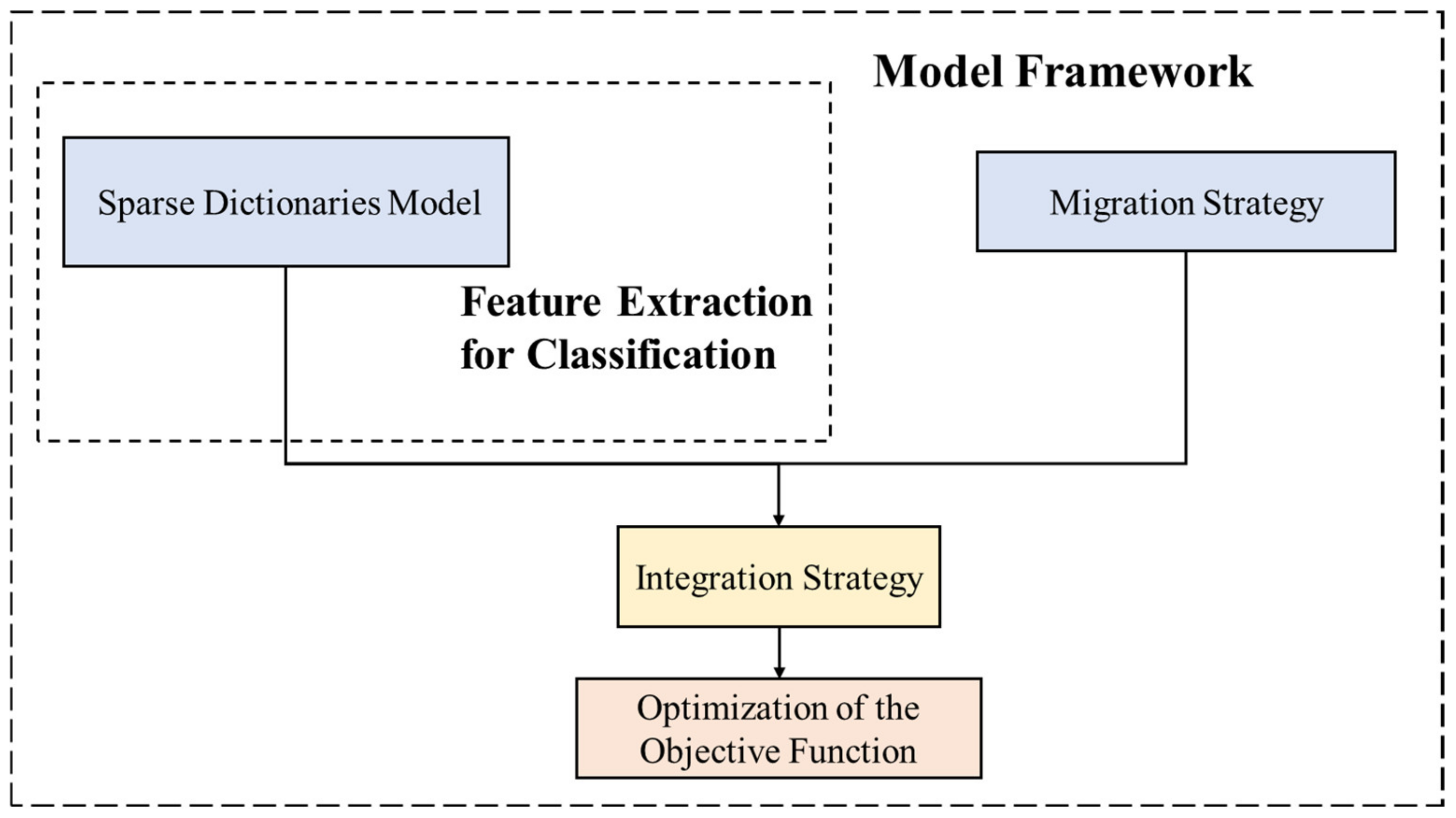
2.1. Model Principle

This study contemplates the amalgamation of the augmented dictionary transfer model and the transfer sparse coding (TSC) model, thereby enabling the transfer learning model to harness the strengths of both. It also takes into account the semi-supervised scenario, to discover the information pertaining to labeled sample categories and to establish a category dictionary augmented transfer learning model suitable for such a scenario. The implementation flow of the migration model is depicted in Figure 1.
Initially, an incremental dictionary model is constructed. Following that, sparse features are extracted from this dictionary model for classification. This extraction process serves to pave the way for future transfer learning operations.
Furthermore, a migration strategy is put forward. With the aim of minimizing the sum of distances, this strategy ensures strong connectivity between the source and target domains for the corresponding sparse coefficients of the labeled samples.
Following that, an integration strategy is designed to migrate the sparse feature coefficients to different data domains. Subsequently, optimization is carried out for the fused objective function.
The underlying principle of the method is illustrated in Figure 2, where the upper (light color) and lower (dark color) figures represent the original data space and the new space generated by the corresponding sparse coefficients, respectively. The different categories in the source domain (target domain) are depicted as triangles (pentagons) and circles (squares). Evidently, the aim of our model (SSDT) is to bring the labeled target domain samples closer to the source domain samples in the new space mapped by the category dictionary through distance constraints. Simultaneously, it introduces category means to mitigate the differences in conditional probability distributions between the original domain and the target domain.

2.2. Common Data Symbols

In alignment with the notation utilized in sparse classification of the relevant category dictionary, X s = [ X 1 s X m s X M s ] d × N s is employed to denote the source domain data matrix, where N s represents the total number of samples within the source domain. The term X m s = [ x 1 , m s , , x i , m s , , x N m s , M s ] d × N m s corresponds to the data matrix of class m in the source domain, with x i , m s denoting individual sample data. The notation X t , l = [ X 1 t , l X m t , l X M t , l ] d × N t , l is used to signify the data matrix composed of the labeled samples in the target domain. X m t , l = [ x 1 , m t , l x j , m t , l x N m t , l , m t , l ] d × N m t , l represents the data matrix of class m in the target domain, where x j , m t , l stands for individual sample data. The notation X t , u d × N t , u corresponds to the data matrix consisting of unlabeled samples in the target domain. I m is used to represent the number of dictionaries corresponding to each class of samples. For any given test sample, D m is employed in lieu of X m as the category dictionary.

2.3. Sparse Dictionaries Model

In the case of data matrices X m s and X m t , l , which are formed by the class m samples x i , m s , x j , m t , l in the source and target domains, the class m data constitution augmentation matrix is represented as X m = [ X m s   X m t , l ] . The representation model of X m in relation to the data matrix can be expressed as:
min D m , S m X m D m S m F 2 + λ 1 S k , m 1
Moreover, taking into account the augmentation strategy delineated in the literature [3], X k , m t , u d × N k , m t , u is employed to denote the data matrix composed of the pseudo-tagged samples selected in the target domain at the kth iteration and classified in class m. Here, N k , m t , u signifies the number of samples per class.
Subsequently, the data matrix X k , m = [ X m s   X m t , l   X k , m t , u ] , the category dictionary matrix D k , m d × I m and the sparse representation coefficients S k , m I m × ( N m s + N m t , l + N k , m t , u ) are defined, respectively. Thus, function (1) can be re-expressed as:
min D k , m , S k , m X k , m D k , m S k , m F 2 + λ 1 S k , m 1
At the k th iteration, the data matrix incremental expression is represented as X k , m t , u = [ X k 1 , m t , u   X ˜ k , m t , u ] , where X ˜ k , m t , u refers to the selected sample of the current iteration. This indicates that the current data matrix builds upon prior results. The matrix denoting class m samples remains unchanged during subsequent selection. The incremental model proposed in this study increases the number of selected target domain samples in each category after every iteration, i.e., N k , m t , u = k N ˜ m t , u , where N ˜ m t , u is a constant, obviating the need for inheritance relationships among the set of selected target domain samples.

2.4. Migration Strategy

In the context of the semi-supervised transfer learning scenario, given that the target domain contains a limited number of labeled samples, the disparity between the source and the target domain can be bridged in each category subspace. Aiming at minimizing the sum of distances, a strong connection is established for the corresponding sparse coefficients of labeled samples in the source and target domains.
Θ ^ m = 1 N m s N m t , l i = 1 N m s j = 1 N m t , l s i , m s s j , m t , l 2 2 = t r [ L i j 2 i = 1 N m s + N m t , l j = 1 N m s + N m t , l ( s i , m s j , m ) ( s i , m s j , m ) T ]
where,
L i j = { 1 ( N m s N m t , l ) , s i , m S m s , s j , m S m t , l 1 ( N m s N m t , l ) , s j , m S m s , s i , m S m t , l 0 ,                                                     o t h e r s
S m s and S m t , l denote the sparse representation coefficients generated from the source domain, target domain labeled samples, respectively.
For ease of mathematical computation, Equation (3) can be further simplified to:
Θ ^ m = 1 2 t r ( S ^ k , m ^ m ° S ^ k , m T )
^ m ° = L d , m L m , L d , m = d i a g ( l 1 , , l N m s + N m t , l ) is a diagonal matrix with diagonal elements equating to the sum of elements in each column of the L d , m matrix. ^ m ° can be considered a Laplacian matrix produced by a symmetric matrix, and S ^ k , m = [ S m s   S m t , l ] . When the value of Θ ^ m is small, it signifies that similar samples in the source and target domains are geometrically closer, thereby reducing the differences between domains.
However, this full linkage presents strong constraints, and when the selected pseudo-tagged samples in the target domain are incorrectly tagged, it can adversely impact the entire model. Further, it may be beneficial to search for information that aids domain migration from the augmented data matrix X ˜ k , m t , u within the target domain, to expand the range of sample applicability within the target domain. In this study, considering the sparse representation coefficients generated by aligning the source domain and target domain sample data in the conditional probability sense, the corresponding mathematical expressions are:
Θ ˘ k , m = 1 N m s i = 1 N m s s i , m s 1 N m t , l + N m t , u ( j = 1 N m t , l s j , m t , l + j = 1 N k , m t , u s j , k , m t , u ) 2 2 = t r [ 1 N m s i = 1 N m s s i , m s 1 N m t , l + N m t , u ( j = 1 N m t , l s j , m t , l + j = 1 N k , m t , u s j , k , m t , u ) ( 1 N m s i = 1 N m s s i , m s 1 N m t , l + N m t , u ( j = 1 N m t , l s j , m t , l + j = 1 N k , m t , u s j , k , m t , u ) ) T ]
To facilitate the calculation, it is defined that S k , m = [ S m s   S m t , l   S m t , u ] . With this definition, the aforementioned equation can be reformulated as follows:
Θ ˘ k , m = t r ( S k , m ˘ k , m S k , m T )
where,
˘ k , m = { 1 ( N m s ) 2 , s i , m , s j , m S m s 1 ( N m t , l + N m t , u ) 2 , s i , m , s j , m S m t , l S k , m t , u 1 N m s ( N m t , l + N m t , u ) , s i , m S m s , s j , m S m t , l S k , m t , u s j , m S m s , s i , m S m t , l S k , m t , u

2.5. Integration Strategy

Combining Equations (6)–(9) gives:
Θ k , m = λ 2 Θ ^ m + λ 3 Θ ˘ k , m = λ 2 2 t r ( S ^ k , m ^ m ° S ^ k , m T ) + λ 3 t r ( S k , m ˘ k , m S k , m T )
where λ 2 and λ 3 are the two given constants.
For convenience, consider expanding S ^ k , m to S k , m and use ˘ k , m to represent the rewritten ^ m ° . Specifically, the corresponding position elements of S m s and S m t , l are set to be zero after each iteration.
min D k , m , S k , m X k , m D k , m S k , m F 2 + λ 1 S k , m 1 + t r ( S k , m Θ k , m S k , m T )
s . t . d i , k , m 2 1 ,   i = 1 , , I m
where d i , k , m 2 1 is guaranteed to indicate that the sparse coefficients obtained by the model are within a reasonable range.

2.6. Optimization of the Objective Function

The optimization objective function shown in Equation (10) contains two variables. To solve this effectively, a distributed optimization solution strategy could be employed. This approach treats one variable as a constant while solving for the other, thereby simplifying the process.

2.6.1. Solve for the Variable S k , m

In solving for the variable D k , m while holding S k , m constant, Equation (10) can be reformulated as follows:
min S k , m X k , m D k , m S k , m F 2 + λ 1 S k , m 1 + t r ( S k , m Θ k , m S k , m T )
This equation consists of three functional terms related to the variable S k , m encompassing both 1 and Frobenius norm operations. Drawing an analogy with the method outlined in the literature [11] (pp. 850–863), the introduction of intermediate variables, denoted as W k , m , can be considered. This leads to the following expression:
min S k , m , W k , m X k , m D k , m S k , m F 2 + λ 1 W k , m 1 + t r ( S k , m Θ k , m S k , m T )
s . t .     S k , m = W k , m
Establishing the multiplicative Lagrange multiplier function on the above equation:
C 1 = X k , m D k , m S k , m F 2 + λ 1 W k , m 1 + t r ( S k , m Θ k , m S k , m T ) + Y 1 , S k , m W k , m + ρ 1 2 ( S k , m W k , m F 2 )
where Y 1 and ρ 1 > 0 are the additional Lagrange multipliers and penalty factors introduced, respectively.
Further using a distribution optimization strategy to solve for the variables in the above equation, first fixing W k , m , the expression with respect to S k , m is:
C 1 1 = X k , m D k , m S k , m F 2 + t r ( S k , m Θ k , m S k , m T ) + ρ 1 2 ( S k , m W k , m F 2 )
Taking the derivative of Equation (14) and making the derivative zero, the following result is obtained.
( 2 D k , m T D k , m + ρ 1 I ) S k , m + S k , m ( 2 Θ k , m ) = 2 D k , m T X k , m + ρ 1 ( W k , m Y 1 ρ 1 )
The above equation is a Sylvester equation [8] for the variable S k , m , and the parameters of the set of equations are: A = ( 2 D k , m T D k , m + ρ 1 I ) , B = 2 Θ k , m , and C = 2 D k , m T X k , m + ρ 1 ( W k , m Y 1 ρ 1 )
Solve the above parameters by matrix analysis (e.g., using the MATLAB integrated function lyap).
Then, fixing the variable S k , m , form the expression of the objective function with respect to the variable W k , m :
C 1 2 = λ 1 W k , m 1 + ρ 1 2 ( S k , m W k , m + Y 1 ρ 1 F 2 )
The optimization problem described by the above equation, i.e., min W k , m C 1 2 has a closed solution and the expression is shown below:
W k , m = s h r i n k ( S k , m + Y 1 ρ 1 , ρ 1 λ 1 )
Finally, update the auxiliary variables in Equation (14):
{ ρ 1 = min ( ρ 1 κ , ρ m a x ) Y 1 = Y 1 + κ ( S k , m W k , m )
where κ is a constant slightly greater than 1.
After that, repeat the process of executing Equations (14)–(18) continuously until the values of the variables to be solved satisfy the given convergence conditions. Then, the above algorithm process is executed separately for each class of samples and dictionaries to obtain the corresponding S k , m and W k , m .

2.6.2. Solve for the Variable D k , m

Fixing S k , m and removing the uncorrelated function term with the variable D k , m , Equation (10) can be rewritten as:
min D k , m X k , m D k , m S k , m F 2         s . t . d i , k , m 2 1 ,   i = 1 , , I m
The method in the literature [12] was chosen to solve for the variable D k , m . The specific process of the algorithm is shown in Algorithm 1.
Algorithm 1: Semi-Supervised Category Dictionary Model Based on Transfer Learning
Input: Dataset X s , X t , l , X t , u ; parameter λ 1 , λ 2 , λ 3 , κ
Output: X t , u corresponding labels
1.Build data matrix X s , X t , l , X t , u . Set k = 0 , Iter = 0 ;
2.For Iter Iter max do
3.    Initialize D 0 , m , ˘ 0 , m , ^ m ° , X m s , X m t , l , X t , u ;
4.    For k k max do
5.  Update S k , m ;
6.   m = 1 ;
7.  For m M do
8.   Initialize ρ 1 , κ , W k , m , Y 1 ;
9.   While 1 do
10.    Calculate the coefficient matrix A , B , C ;
11.    Update S k , m according to Equation (15);
12.    Update W k , m according to Equation (17);
13.    Update ρ 1 and Y 1 according to Equation (18);
14.    If meet the termination conditions then
15.     Break
16.    End if
17.   End
18.  End
19.  For m M do
20   Update D k , m according to Equation (19);
21.  End
22.   k = k + 1 ;
23.    End
24.    Based on the dictionary D k , m , X t , u corresponding expression coefficients and category residuals are obtained.;
25.    Transform X t , u into the corresponding discrete probability values for each category of residuals and obtain the pseudolabel;
26.    The N ˜ m t , u pseudo-labeled samples with larger probability values within the subcategory are selected to form X k , m t , u ;
27.    Update X k , m ;
28.    Iter = Iter + 1
29.End

3. Experiments and Results Analysis

3.1. Analysis Object

Two experiments were designed to test the accuracy of SSDT.

3.1.1. Data of Vision

For the first experiment, in line with the experimental setup proposed by reference [13], this study contemplates employing the three visual recognition repositories, namely SUN09 [14], VOC2007 [15], and LabelMe [16], as test datasets to establish a cross-domain learning task. It is noteworthy that these visual recognition datasets have been extensively adopted to validate the performance of various transfer learning models [17,18,19], encompassing five shared categories, such as people, cars, etc. In particular, the datasets of SUN09, VOC2007, and LabelMe comprise 3282, 3376, and 2656 samples, respectively.
Throughout the experiment, the preprocessed image features released by Fang et al. are utilized [13,20]. These features are extracted from the raw data through the application of multilayer convolutional neural networks (CNNs) [21,22]. For each sample, two distinct forms of features are incorporated, including the output of the sixth fully connected layer (fc6) and the output of the seventh fully connected layer (fc7).

3.1.2. Data of Bearing Fault Diagnosis

For the second experiment, the experimental data employed in this study were procured from the Bearing Data Center at Case Western Reserve University. As depicted in Figure 3, the bearing failure experimental platform comprises induction motors, torque sensors, linkage devices, and electronic controllers, among other components [23]. An acceleration sensor, attached to the housing, is used to capture vibration data at a sampling frequency of 12 kHz. The fan load can be adjusted to different horsepower (hp). Faults manifest in the inner ring, outer ring, and the rolling body, each with varying levels of degradation depth. Figure 4 presents the waveform of the vibration signal captured in the inner ring failure mode in the dataset, demonstrating irregular fluctuations. Due to the complex operational environment of rolling bearings, the data not only encapsulate intrinsic fault information, but also capture the vibration information generated by other rotating mechanical parts, along with their noise.
The bearing failure dataset from Case Western Reserve University was utilized for this study, where load magnitude served as a control parameter for constructing the source and target domain datasets. Data under no-load conditions, encompassing normal and fault states, were designated as the source domain. This domain includes four categories: normal, inner ring fault, rolling element fault, and outer ring fault, each featuring multiple degradation depths. Addressing the issue of ultra-long vibration data in fault diagnosis, the original data were segmented into multiple data blocks based on a specified length. In the conducted experiment, the sample length was set to 1100. To mitigate boundary effects caused by truncation, and ensuring an overlap between different data blocks [24], the overlap length was set to 60. Prior to these operations, the sample data underwent normalization.
In order to facilitate a comprehensive comparison of the performance of various models, mean, standard deviation, and maximum values were computed for the bearing fault diagnosis task. These measures, obtained by conducting 10 repetitions, served as the performance indices. Under no-load conditions, 200 samples from each category, amounting to a total of 800 labeled samples, were curated to generate the source domain dataset. Under a 3 horsepower load condition, 10 samples from each category, summing up to 40 labeled samples, were selected to constitute a small number of labeled samples in the semi-supervised target domain. The remaining 1477 samples were utilized as the test set in the target domain.

3.2. Model Settings

For the sake of convenience, and following the conventions in references [13], S, V, and L are used to represent the SUN09, VOC2007, and LabelMe datasets, respectively. Meanwhile, the symbol S→V denotes the cross-domain transfer learning task. Considering the characteristics of each dataset, the transfer learning tasks are established with the following settings:
  • When LabelMe is the source domain, 65 labeled samples are randomly selected per category, resulting in a total of 302 samples. Sun09 and VOC2007 serve as target domains where three labeled samples are chosen at random, constituting an aggregate of 15 samples. The remaining samples in the target domains are used as the test set, and the dictionary size for each category is Im = 35;
  • When Sun09 serves as the source domain, 30 labeled samples are randomly selected per category, totaling 140 samples. LabelMe and VOC2007 act as the target domains, with the allocation of labeled samples and test sets remaining identical to the aforementioned settings. The dictionary size for each category is Im = 20;
  • When VOC2007 is employed as the source domain, 65 labeled samples are randomly selected per category, amassing 325 samples in total. LabelMe and Sun09 function as target domains, maintaining the same configuration of labeled samples and test sets as previously described. The dictionary size for each category is Im = 35.
Utilize 1-NN [25], SRC [26], TSC [4] and LSDT [27] as the comparative models.
The 1-NN model is an example of supervised learning, while SRC models involving coefficient feature extraction, followed by supplementary classification strategies, also fall under the category of supervised learning. Additionally, LSDT, TSC, TCA, and GFK are all considered domain adaptation models. Due to their transfer learning nature, these models migrate models applicable to one data domain to a new data domain. Since some one-to-one correspondence needs to be confirmed during the migration process, these models are considered to be semi-supervised during the migration process.
For our model (SSDT), λ 1 = 0.05 , λ 2 = 0.04 , λ 3 = 0.01 , the number of category magnitude dictionaries is 150, the number of augmented samples for each category in each iteration N ˜ m t , u = 3 , and the maximum number of iterations is set to 8. The specific flow of the model is shown in Figure 5.

3.3. Results Analysis

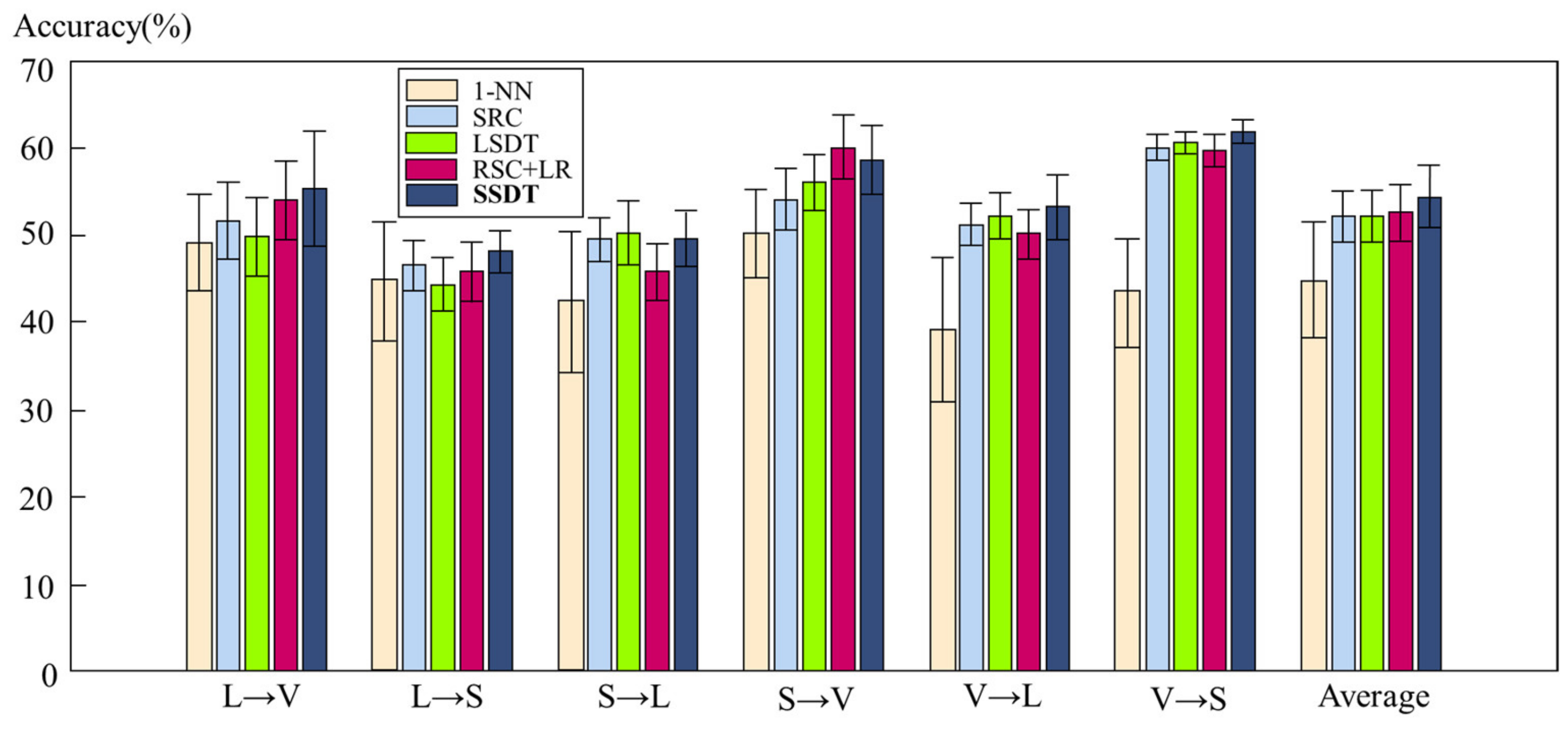
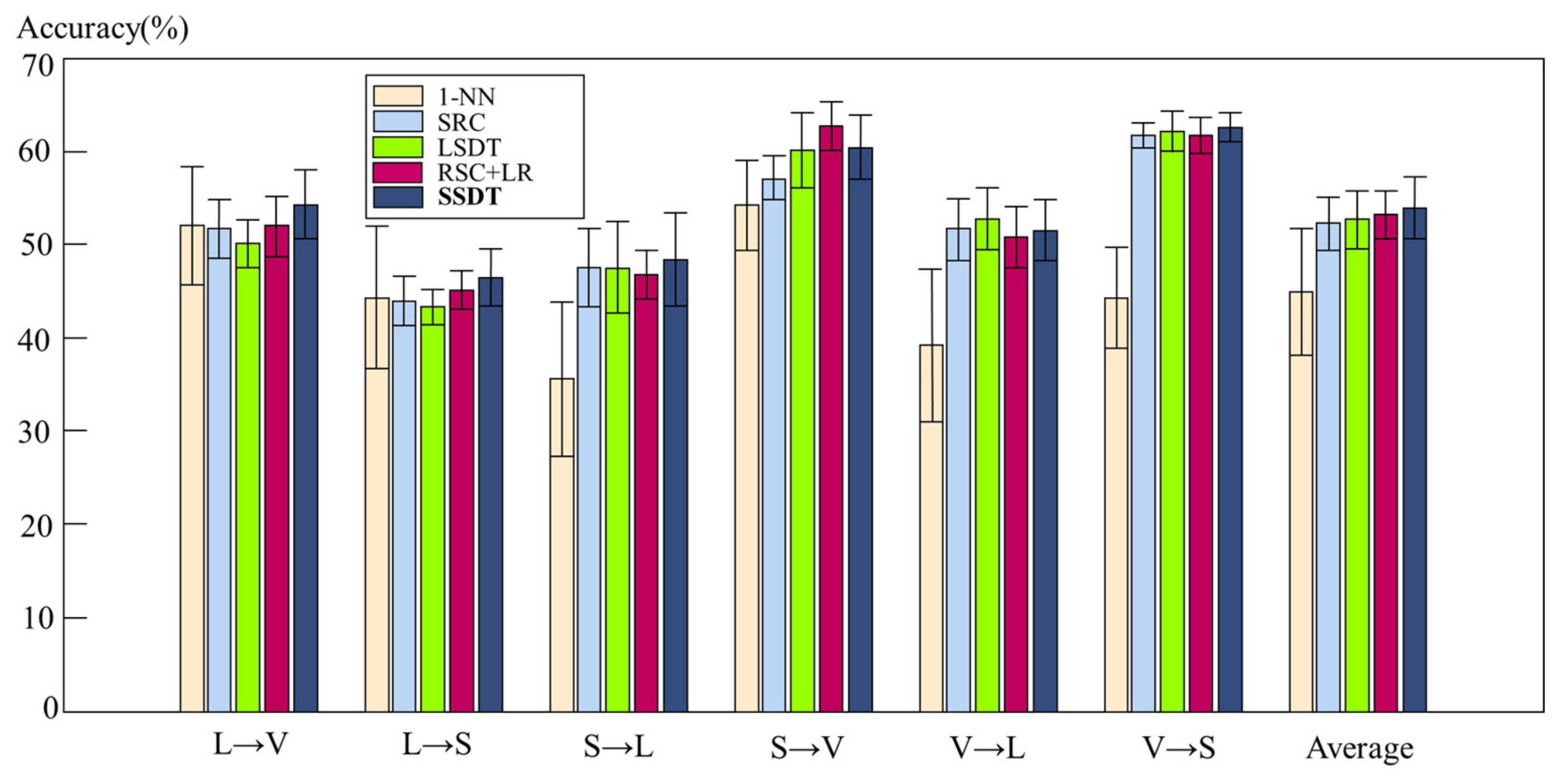
3.3.1. Results Analysis of the Vision Data Experiment

Utilizing the cross-domain mixed datasets introduced earlier, six cross-domain transfer learning tasks can be established.
To make the experimental results statistically more significant, each transfer learning task is repeated ten times, with mean, standard deviation, and maximum values selected as indicators to compare the performance of different methods. The experimental results, based on the output features of the sixth hidden layer (fc6) are shown in Table 1 and Table 2. It can be observed that, among all comparative methods, the category dictionary augmented transfer learning model demonstrates the best overall performance. In four out of six transfer tasks, the model achieves the highest classification accuracy in terms of mean value, while also attaining the best results for maximum values in three classification tasks. For a better visualization of the model’s performance, bar charts of data from Table 1 and Table 2 are depicted in Figure 6 and Figure 7, respectively.
Comparing the experiments with a 1-NN model, it is apparent that, despite containing a limited number of labeled samples in the target domain, relying solely on existing labels within the target domain does not enable the classifier to achieve good generalization ability overall. Although the 1-NN model may yield satisfactory classification results in some scenarios, its output exhibits significant fluctuations due to variances. Introducing source domain samples to assist in completing target domain classification tasks has a positive effect on enhancing classifier generalization performance.
In the experiments, the transfer learning models (LSDT, TSC) exhibit improved classification performance compared to non-transfer learning models (1-NN, SRC). This indicates that incorporating cross-domain transfer operations contributes to the integration of source and target domain data, promoting efficient utilization. In summary, compared to baseline methods, the category dictionary augmented transfer learning model demonstrates stronger competitiveness in performance. This is partly attributed to inheriting the SRC, and the strategies in the literature that propose using category dictionaries for residual reconstruction to complete label predictions without introducing additional classifiers. Furthermore, the model establishes strong correlation constraints between source and target domains based on limited labeled samples in the target domain, using conditional probability distribution to facilitate knowledge transfer across different domains.
The experimental results based on the output features of the seventh hidden layer (fc7) are presented in Table 3 and Table 4. Similar to the outcomes with fc6 features, the category dictionary augmented transfer learning model exhibits the most exceptional overall performance among all experimental methods. The model’s mean value achieves the best results in the L→V, L→S, V→L, and V→S transfer tasks, while the maximum values obtain the best outcomes in the L→V, V→L, and V→S transfer tasks. Furthermore, LSDT and TSC models perform best in the S→L and S→V cross-domain tasks, respectively. In the remaining cross-domain tasks, they outperform SRC and 1-NN models. These findings reiterate that the introduction of auxiliary domain data can indeed improve model performance compared to non-transfer classifiers.
For a better visualization of the model’s performance, bar charts of data from Table 3 and Table 4 are depicted in Figure 8 and Figure 9, respectively.

3.3.2. Results Analysis of Bearing Fault Diagnosis Data Experiment

Four classifiers, 1-NN, SRC, TCA [9] and GFK [10], were selected as comparison benchmarks to validate the effectiveness of the SSDT model in bearing fault diagnosis.
In the case of the SRC model, the sparse regularization parameter was set to 0.1. The procedure for the SRC model, as outlined in the literature [28], was employed in the experiments. This involves the use of a fast l^1 optimization algorithm [29] to solve for the sparse representation coefficients.
For the GFK model, set the subspace dimension d   =   350 .
For the TCA model, set the subspace dimension d   =   200 and the regularization parameter μ   =   0.1 .
The experimental results of the SSDT model in the bearing fault diagnosis process are presented in Table 5 and Figure 10. These results show that the SSDT model yields the highest correct classification rate (highlighted in bold) in terms of both average and maximum values. This represents a significant performance improvement in comparison to 1-NN, SRC, GFK, and TCA, suggesting that the SSDT model is also suitable for the bearing fault diagnosis task.
An examination of the impact of iteration count on the performance of the SSDT model is presented via a variation curve of the accuracy rate with respect to the number of iterations in Figure 11. The observed positive correlation between the number of augmentation iterations and the correct classification rate suggests that incorporating a category dictionary-based reconstruction of residual sample augmentation operation contributes to enhancing the model’s generalization performance.
Comparative experiments involving the 1-NN model demonstrated considerable fluctuations in the output results, as indicated by the variance values. Despite the presence of a modest number of labeled samples in the target domain, the limited sample size, relying solely on existing labels in the target domain, generally precludes the classifier from achieving robust generalization ability. This suggests that the inclusion of source domain samples to aid in target domain classification tasks can effectively enhance the generalization performance of the classifier.
It is worth noting that the calculation time difference between different methods is not significant. In a regular configuration computer, the calculation time is usually a few seconds. Therefore, the proposed method is meaningful for improving accuracy when the calculation time is not significantly different.

4. Conclusions

For cross-domain transfer tasks involving a limited number of labeled samples within the target domain, a semi-supervised category dictionary augmentation transfer learning model is proposed. This study presents a semi-supervised category dictionary augmentation transfer learning model, developed on the foundation of existing category dictionary sparse representation classification and dictionary transfer methods. This model is based on TSC and augmented dictionary domain adaptation, performing confident sample selection in each iteration using category reconstruction error as the criterion.
This study presents a semi-supervised category dictionary augmentation transfer learning model, developed on the foundation of existing category dictionary sparse representation classification and dictionary transfer methods. By employing the 1 parameter as the sparse representation constraint, the model unifies the conditional probability distribution and intra-class sample distance to construct the total objective function. This model, compared to the transfer sparse coding (TSC) approach, does not necessitate the additional design of classifiers, and is adept at leveraging labeled sample class information.
To further bridge the gap between different domains, residuals are reconstructed based on unlabeled target domain samples on the category representation dictionary to procure sample labels. Moreover, a specific number of target domain samples are chosen in each iteration, based on the normalized discrete probability distribution in each class of pseudo-labeled samples. These samples are then amalgamated with source domain samples to generate an augmented data matrix. With the use of a step-by-step solution strategy, the category dictionary is established alongside the sparse representation coefficient update formula to attain an optimal solution.
The applicability of the proposed model is evaluated through its implementation in a real-world bearing fault diagnosis. For comparative analysis, migration and non-migration models such as 1-NN and SRC serve as benchmarks to gauge the classification effectiveness of each model. Based on the evaluation results, the proposed model demonstrated superior performance compared to the benchmark models, achieving higher average correct classification rates and maximum values.

Author Contributions

Conceptualization, Y.D. and H.Y.; methodology, Y.D. and B.Z.; software, Y.L. and H.S.; validation, H.S. and B.Z.; investigation, H.Y.; data curation, B.H.; writing—original draft preparation, Y.L.; writing—review and editing, H.S.; supervision, Y.D. All authors have read and agreed to the published version of the manuscript.

Funding

This research was funded by Science and Technology project of State Grid Corporation: Research and application of insulator string digitization for UHV transmission line based on multi-parameter composite perception, grant number 520950220005.

Institutional Review Board Statement

Not applicable.

Informed Consent Statement

Not applicable.

Data Availability Statement

The experimental data employed in this study were procured from the Bearing Data Center at Case Western Reserve University. Bearing test data. Case Western Reserve University Bearing Data Center [30].

Acknowledgments

Yingyi Liu and Haoyu Song are corresponding authors. This research was supported by Science and Technology project of State Grid Corporation: Research and application of insulator string digitization for UHV transmission line based on multi-parameter composite perception (520950220005).

Conflicts of Interest

The authors declare no conflict of interest.

References

  1. Shekhar, S.; Patel, V.M.; Nguyen, H.V.; Chellappa, R. Generalized domain-adaptive dictionaries. In Proceedings of the IEEE Conference on Computer Vision and Pattern Recognition, Portland, OR, USA, 23–28 June 2013; pp. 361–368. [Google Scholar]
  2. Pan, S.J.; Yang, Q. A Survey on Transfer Learning. IEEE J. Mag. 2010, 22, 1345–1359. Available online: https://ieeexplore.ieee.org/document/5288526 (accessed on 2 February 2023).
  3. Lu, B.; Chellappa, R.; Nasrabadi, N.M. Incremental Dictionary Learning for Unsupervised Domain Adaptation. In Proceedings of the British Machine Vision Conference 2015, Swansea, UK, 7–10 September 2015; British Machine Vision Association: Swansea, UK, 2015; pp. 108.1–108.12. [Google Scholar]
  4. Long, M.; Ding, G.; Wang, J.; Sun, J.; Guo, Y.; Yu, P.S. Transfer Sparse Coding for Robust Image Representation. In Proceedings of the 2013 IEEE Conference on Computer Vision and Pattern Recognition, Portland, OR, USA, 23–28 June 2013; pp. 407–414. [Google Scholar]
  5. Supervised Transfer Sparse Coding. In Proceedings of the AAAI Conference on Artificial Intelligence, held virtually, 22 February–1 March 2022; Available online: https://ojs.aaai.org/index.php/AAAI/article/view/8981 (accessed on 2 February 2023).
  6. Wang, S.; Zhang, L.; Zuo, W. Class-Specific Reconstruction Transfer Learning via Sparse Low-Rank Constraint. In Proceedings of the 2017 IEEE International Conference on Computer Vision Workshops (ICCVW), Venice, Italy, 22–29 October 2017; pp. 949–957. [Google Scholar]
  7. Pereira, L.A.; da Silva Torres, R. Semi-supervised transfer subspace for domain adaptation. Pattern Recognit. 2018, 75, 235–249. [Google Scholar] [CrossRef]
  8. Ding, Z.; Shao, M.; Fu, Y. Latent Low-Rank Transfer Subspace Learning for Missing Modality Recognition. In Proceedings of the Twenty-Eighth Aaai Conference on Artificial Intelligence, Québec City, QC, Canada, 27–31 July 2014; Assoc Advancement Artificial Intelligence: Palo Alto, CA, USA, 2014; pp. 1192–1198. [Google Scholar]
  9. Pan, S.J.; Tsang, I.W.; Kwok, J.T.; Yang, Q. Domain Adaptation via Transfer Component Analysis. In Proceedings of the 21st International Joint Conference on Artificial Intelligence (ijcai-09), Pasadena, CA, USA, 11–17 July 2009; Boutilier, C., Ed.; Ijcai-Int Joint Conf Artif Intell: Freiburg, Germany, 2009; pp. 1187–1192. [Google Scholar]
  10. Gong, B.; Shi, Y.; Sha, F.; Grauman, K. Geodesic Flow Kernel for Unsupervised Domain Adaptation. In Proceedings of the 2012 Ieee Conference on Computer Vision and Pattern Recognition (cvpr), Providence, RI, USA, 16–21 June 2012; IEEE: New York, NY, USA, 2012; pp. 2066–2073. [Google Scholar]
  11. Xu, Y.; Fang, X.; Wu, J.; Li, X.; Zhang, D. Discriminative Transfer Subspace Learning via Low-Rank and Sparse Representation. IEEE Trans. Image Process. 2016, 25, 850–863. [Google Scholar] [CrossRef] [PubMed]
  12. Lee, H.; Battle, A.; Raina, R.; Ng, A. Efficient sparse coding algorithms. In Proceedings of the Advances in Neural Information Processing Systems; MIT Press: Cambridge, MA, USA, 2006; Volume 19. [Google Scholar]
  13. Fang, C.; Xu, Y.; Rockmore, D.N. Unbiased metric learning: On the utilization of multiple datasets and web images for softening bias. In Proceedings of the IEEE International Conference on Computer Vision, Sydney, Australia, 1–8 December 2013; pp. 1657–1664. [Google Scholar]
  14. Choi, M.J.; Lim, J.J.; Torralba, A.; Willsky, A.S. Exploiting hierarchical context on a large database of object categories. In Proceedings of the 2010 IEEE Computer Society Conference on Computer Vision and Pattern Recognition, San Francisco, CA, USA, 13–18 June 2010; pp. 129–136. [Google Scholar]
  15. Everingham, M.; Van Gool, L.; Williams, C.K.; Winn, J.; Zisserman, A. The pascal visual object classes (voc) challenge. Int. J. Comput. Vis. 2010, 88, 303–338. [Google Scholar] [CrossRef] [Green Version]
  16. Russell, B.C.; Torralba, A.; Murphy, K.P.; Freeman, W.T. LabelMe: A database and web-based tool for image. Int. J. Comput. Vis. 2005, 77, 157–173. [Google Scholar] [CrossRef]
  17. Tommasi, T.; Tuytelaars, T. A testbed for cross-dataset analysis. In Proceedings of the Computer Vision-ECCV 2014 Workshops, Zurich, Switzerland, 6–7, 12 September 2014; Proceedings Part III 13. Springer: Berlin/Heidelberg, Germany, 2015; pp. 18–31. [Google Scholar]
  18. Ding, Z.; Fu, Y. Deep domain generalization with structured low-rank constraint. IEEE Trans. Image Process. 2017, 27, 304–313. [Google Scholar] [CrossRef] [PubMed]
  19. Ghifary, M.; Kleijn, W.B.; Zhang, M.; Balduzzi, D. Domain generalization for object recognition with multi-task autoencoders. In Proceedings of the IEEE International Conference on Computer Vision, Santiago, Chile, 7–13 December 2015; pp. 2551–2559. [Google Scholar]
  20. Data of Vision. Available online: https://www.cs.dartmouth.edu/~chenfang/%20proj_page/FXR_iccv13/%20index.%20php (accessed on 14 May 2023).
  21. Krizhevsky, A.; Sutskever, I.; Hinton, G.E. Imagenet classification with deep convolutional neural networks. Commun. ACM 2017, 60, 84–90. [Google Scholar] [CrossRef] [Green Version]
  22. Donahue, J.; Jia, Y.; Vinyals, O.; Hoffman, J.; Zhang, N.; Tzeng, E.; Darrell, T. DeCAF: A Deep Convolutional Activation Feature for Generic Visual Recognition. In Proceedings of the International Conference on Machine Learning, Beijing, China, 21–26 June 2014; pp. 647–655. [Google Scholar]
  23. Liu, H.; Liu, C.; Huang, Y. Adaptive feature extraction using sparse coding for machinery fault diagnosis. Mech. Syst. Signal Process. 2011, 25, 558–574. [Google Scholar] [CrossRef]
  24. Lu, W.; Liang, B.; Cheng, Y.; Meng, D.; Yang, J.; Zhang, T. Deep Model Based Domain Adaptation for Fault Diagnosis. IEEE Trans. Ind. Electron. 2017, 64, 2296–2305. [Google Scholar] [CrossRef]
  25. Wang, Y.; Zhou, Z.; Zhou, A. Machine Learning and Its Applications; Tsinghua University Press Co.: Beijing, China, 2006; Volume 4. [Google Scholar]
  26. Wright, J.; Yang, A.Y.; Ganesh, A.; Sastry, S.S.; Ma, Y. Robust Face Recognition via Sparse Representation. IEEE Trans. Pattern Anal. Mach. Intell. 2009, 31, 210–227. [Google Scholar] [CrossRef] [PubMed] [Green Version]
  27. Shao, M.; Castillo, C.; Gu, Z.; Fu, Y. Low-rank transfer subspace learning. In Proceedings of the 2012 IEEE 12th International Conference on Data Mining, IEEE, Washington, DC, USA, 10 December 2012; pp. 1104–1109. [Google Scholar]
  28. Xu, Y.; Li, Z.; Yang, J.; Zhang, D. A Survey of Dictionary Learning Algorithms for Face Recognition. IEEE Access 2017, 5, 8502–8514. [Google Scholar] [CrossRef]
  29. Yang, A.Y.; Sastry, S.S.; Ganesh, A.; Ma, Y. Fast ℓ1-minimization algorithms and an application in robust face recognition: A review. In Proceedings of the 2010 IEEE International Conference on Image Processing, Hong Kong, China, 26–29 September 2010; pp. 1849–1852. [Google Scholar]
  30. Bearing Test Data. Case Western Reserve University Bearing Data Center. Available online: http://csegroups.case.edu/bearingdatacenter/home (accessed on 29 May 2023).
Figure 1. Implementation process of migration model.
Applsci 13 07841 g001
Figure 2. Principle diagram of SSDT.
Applsci 13 07841 g002
Figure 3. Bearing fault diagnosis platform structure schematic diagram.
Applsci 13 07841 g003
Figure 4. Bearing vibration data under inner ring failure (without load).
Applsci 13 07841 g004
Figure 5. SSDT model-based bearing fault diagnosis process.
Applsci 13 07841 g005
Figure 6. Comparison of the average performance of each model based on the cross-domain dataset fc6 layer depth feature.
Applsci 13 07841 g006
Figure 7. Comparison of the best performance of each model based on cross-domain dataset fc6 layer depth features.
Applsci 13 07841 g007
Figure 8. Comparison of the average performance of each model, based on the cross-domain dataset fc7 layer depth feature.
Applsci 13 07841 g008
Figure 9. Comparison of the best performance of each model, based on cross-domain dataset fc7 layer depth features.
Applsci 13 07841 g009
Figure 10. Comparison of the performance of the models on the migration task in the field of bearing fault diagnosis.
Applsci 13 07841 g010
Figure 11. Variation curve of model performance with the number of iterations.
Applsci 13 07841 g011
Table 1. Experimental output of each model, based on cross-domain dataset fc6 layer depth features (mean ± standard deviation %). (The best results for different tasks are bolded).
Task1-NN [25]SRC [26]LSDT [27]TSC + LR [4]SSDT
L→V49.12 ± 5.5851.71 ± 4.4849.80 ± 4.4953.96 ± 4.5155.37 ± 6.59
L→S44.69 ± 6.8746.52 ± 2.9244.42 ± 3.0345.83 ± 3.4548.14 ± 2.38
S→L42.40 ± 8.1149.51 ± 2.4850.31 ± 3.6745.73 ± 3.2749.58 ± 3.21
S→V50.20 ± 5.0954.13 ± 3.5556.04 ± 3.1760.14 ± 3.6258.57 ± 4.00
V→L39.13 ± 8.3051.24 ± 2.4352.27 ± 2.6350.11 ± 2.8153.19 ± 3.74
V→S43.43 ± 6.2460.07 ± 1.4860.57 ± 1.1859.75 ± 1.8561.85 ± 1.38
Average44.83 ± 6.7052.20 ± 2.8952.23 ± 3.0352.59 ± 3.2554.45 ± 3.55
Table 2. Experimental output of each model, based on cross-domain dataset fc6 layer depth features (max %). (The best results for different tasks are bolded).
Task1-NN [25]SRC [26]LSDT [27]TSC + LR [4]SSDT
L→V60.9958.6155.8863.2863.88
L→S52.8049.9848.0351.3651.39
S→L56.7652.4055.6649.4153.96
S→V57.1858.8260.8264.7764.27
V→L46.4654.9855.4755.8558.80
V→S53.5762.6061.9562.7563.45
Average54.6356.2356.3057.9059.29
Table 3. Experimental output of each model, based on cross-domain dataset fc7 layer depth features (mean ± standard deviation %). (The best results for different tasks are bolded).
Task1-NN [25]SRC [26]LSDT [27]TSC + LR [4]SSDT
L→V52.15 ± 6.3951.82 ± 3.1350.24 ± 2.4952.11 ± 3.2654.48 ± 3.69
L→S44.44 ± 7.6344.11 ± 2.6843.43 ± 1.9045.31 ± 2.0446.62 ± 3.03
S→L35.47 ± 8.2647.67 ± 4.2147.72 ± 4.9346.90 ± 2.6048.59 ± 4.95
S→V54.37 ± 4.8057.30 ± 2.3460.27 ± 4.0362.87 ± 2.6460.62 ± 3.42
V→L39.32 ± 8.2251.74 ± 3.3852.94 ± 3.3551.03 ± 3.2551.69 ± 3.30
V→S44.41 ± 5.4261.87 ± 1.3762.33 ± 2.1561.90 ± 1.9462.77 ± 1.52
Average45.07 ± 6.7952.42 ± 2.8552.82 ± 3.1453.35 ± 2.6254.13 ± 3.32
Table 4. Experimental output of each model, based on cross-domain dataset fc7 layer depth features (max %). (The best results for different tasks are bolded).
Task1-NN [25]SRC [26]LSDT [27]TSC + LR [4]SSDT
L→V 61.0257.6953.4757.4261.74
L→S55.8648.0046.7448.3951.70
S→L48.4751.0453.0950.7854.71
S→V62.9362.0465.9066.5066.97
V→L57.0657.1857.2955.0556.83
V→S53.2365.0466.7965.3865.78
Average56.4356.8357.2157.3559.62
Table 5. Comparison of the experimental results. (The best results for different tasks are bolded).
Value1-NN [25]SRC [26]GFK [10]TCA [9]SSDT
Average62.28 ± 1.8886.69 ± 0.7279.95 ± 1.2775.88 ± 0.6587.40 ± 0.90
Maximum71.7288.2281.4577.0589.51
Disclaimer/Publisher’s Note: The statements, opinions and data contained in all publications are solely those of the individual author(s) and contributor(s) and not of MDPI and/or the editor(s). MDPI and/or the editor(s) disclaim responsibility for any injury to people or property resulting from any ideas, methods, instructions or products referred to in the content.

