Learning to Segment Blob-like Objects by Image-Level Counting

Abstract

There is a high demand for manually annotated data in many of the segmentation tasks based on neural networks. Selecting objects pixel by pixel not only takes much time, but it can also lead to inattentiveness and to inconsistencies due to changing annotators for different datasets and monotonous work. This is especially, but not exclusively, the case with sensor data such as microscopy imaging, where many blob-like objects need to be annotated. In addressing these problems, we present a weakly supervised training method that uses object counts at the image level to learn a segmentation implicitly instead of relying on a pixelwise annotation. Our method uses a given segmentation network and extends it with a counting head to enable training by counting. As part of the method, we introduce two specialized losses, contrast loss and morphological loss, which allow for a blob-like output with high contrast to be extracted from the last convolutional layer of the network before the actual counting. We show that similar high F1-scores can be achieved with weakly supervised learning methods as with strongly supervised training; in addition, we address the limitations of the presented method.

1. Introduction

Image segmentation is a common task in deep learning, but it typically involves time-consuming manual annotation work. Usually, it becomes necessary to outline polygons around each object by hand on a large number of images. This not only creates much work, but it also causes inconsistencies in the annotation characteristics, e.g., in the case of unsharp boundaries between objects and the background. This is especially the case when multiple annotators are involved as interobserver variability and, thus, different annotation characteristics may occur. Even if the annotator remains the same, deviations due to intraobserver variabilities cannot be excluded [1]. Existing solutions for training a segmentation with weak supervision are intended for classifications and not for counting [2] as they not only use the pure number of objects, but also use additional information like key points or density maps [3] (or rely on pre-trained encoders, which have to be available for the domain of application or have to be trained beforehand with strong supervision [4]). A straightforward candidate for a solution is to use class activation mapping (CAM) [5] to obtain segmentations from a counting network. In using a self-developed CAM-based approach, we show that this methodology is unsuitable when applied to real data since it does not allow for the controlling of the extracted segmentation shapes. We introduce a counting head, which we constructed as an extension of a segmentation network to enable the counting of objects. To prevent such problems, we developed a weakly supervised segmentation approach, based on specialized loss functions, which corrects undesired segmentation shapes during the training phase. It requires no input other than the expected number of objects in an image, and it does not rely on pre-trained encoders. This training method allows for an annotator to specify the number of objects in an image instead of having to mark the object regions. In this way, manual effort is reduced significantly, and inconsistencies, which can occur with localized annotation, are prevented. We saw advantages in use cases where a large number of objects with unsharp boundaries are to be segmented. This holds particularly for microscopy techniques like fluorescence microscopy [6], bright-field microscopy [7], and surface plasmon resonance imaging (SPRi) [8]. For our studies, we used the image data from the plasmon-assisted microscopy of nano-objects (PAMONO) sensor [9], an SPRi sensor for the detection of viruses and virus-like particles in a biological sample. Annotating the data recorded by this sensor is a monotonous task as it “can take up to one week to label a large data set with high virus concentration” [10], which, thus, makes the obtained annotations person-dependent and potentially inaccurate. We used these data to evaluate our training method from a practical point of view. As a complement to the natural data that were only available in limited numbers, as well as due to the fact that annotations may contain errors and inconsistencies, we also used synthetic data generation for our evaluation. This addition has an advantage in the fact that the images are available in an arbitrary number, the annotations are always consistent, and the number of objects is adjustable. Thus, the evaluation of the synthetic case indicates the achievable results in a controlled environment.

In brief, the main contributions of this paper are as follows:

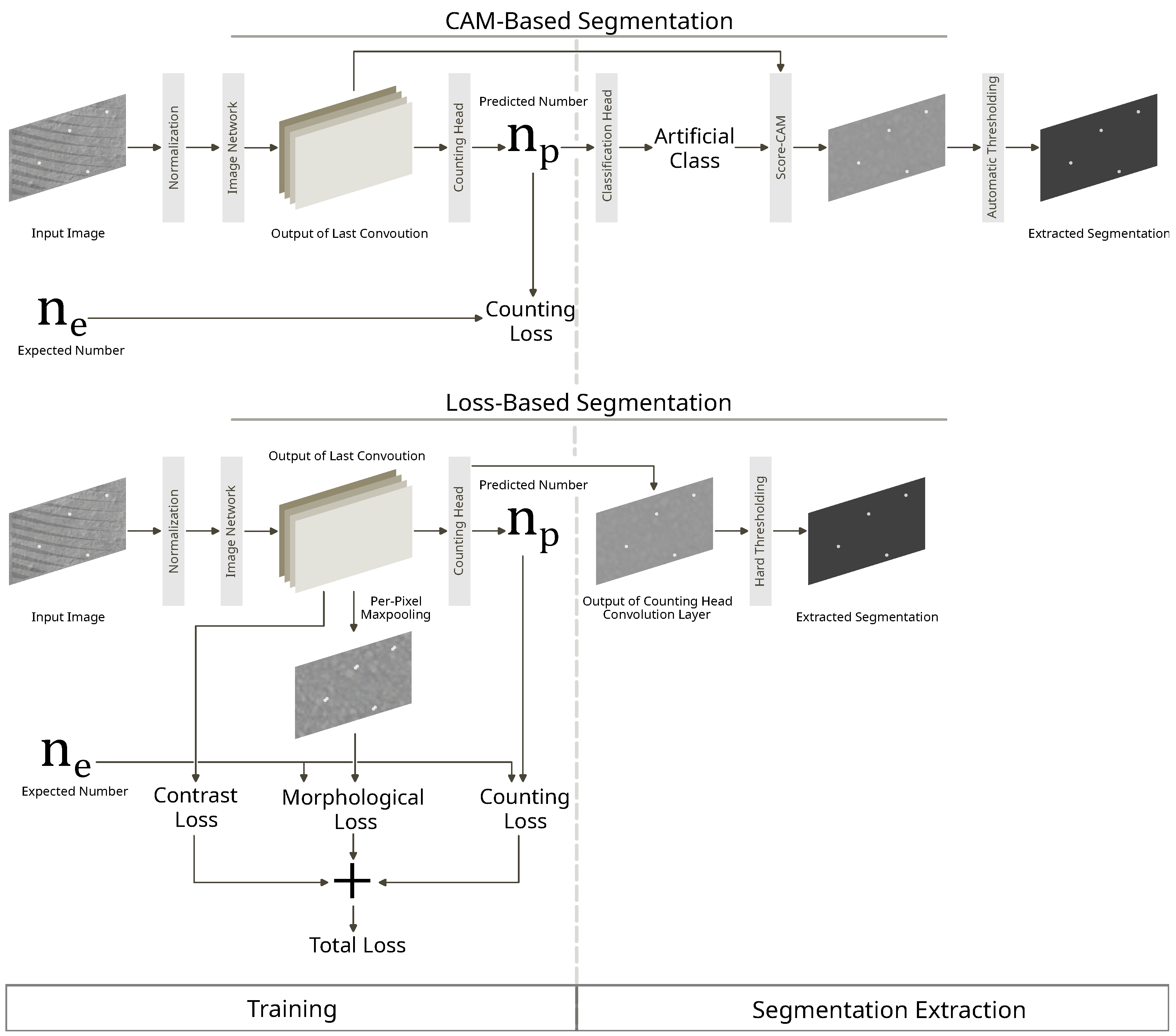
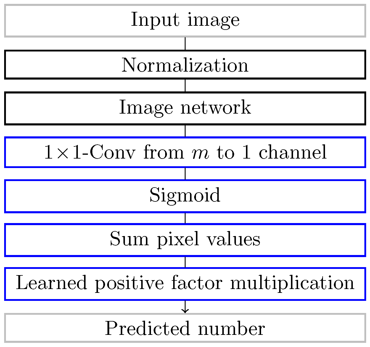
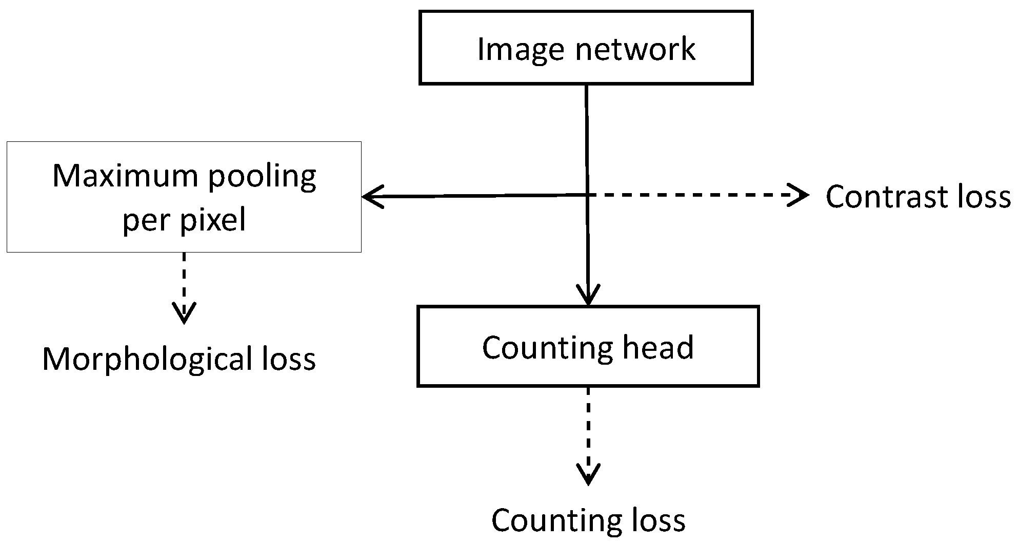
• The development of a counting head as an extension that enables count training for segmentation networks;
• The introduction of a method to connect counting networks to classification-based CAM analysis without losing the counting information;
• The development of two losses, contrast loss and morphological loss, which enforce the outputs of a segmentation learned by count training to be suitable for subsequent blob detection by penalizing noise and favoring blob-like structures.

The structure of this manuscript is as follows: In Section 2, we give a rough overview of the state-of-the-art research in implicit segmentation learning based on image-level classification, address approaches related to object counting, and give examples of image segmentation networks. The methods used for implicit segmentation learning, including the different network architectures to be evaluated, are detailed in Section 3. Section 4 describes the characteristics of the natural and the synthetic image data that were used for the evaluation of the training methods, the experiments performed, and the results of the evaluation (including the undesired effects that emerge from weakly supervised learning). In Section 5, we discuss the results and the gained insights. Finally, we outline aspects that should be investigated further in Section 6.

2. State-of-the-Art Research

An early work dealing with the possibility of training object localization indirectly with a classification task found that the locations of objects can be approximated in a weakly supervised manner [11]. As a drawback, they noticed a poor determination of the extent of the localized objects.

More recent work has presented a network architecture and loss functions for weakly supervised training through image-level classifications [4]. The architecture relies on the pre-trained convolutional layers of a VGG16 [12] network as the encoder part, which is kept frozen and, therefore, relies on the knowledge that was acquired in previous strong supervision training. Although the approach yields good results in segmenting common photos with known object classes, the transfer of the technique is limited to domains where a strong basis in the form of pre-trained networks as encoders is available. In contrast, we targeted an approach that does not rely on this prerequisite. Since the general functionality could be shown for a classification task, we present and evaluated a training method for image-level counting as an annotation for cases with potentially high numbers of objects, and we, then, applied it to different types of network architectures.

A similar field of application is in crowd counting, in which the number of people present in images showing crowds is to be determined. Due to a large number of possible use cases, this topic has attracted great attention in recent years [2,3,13]. Most of the crowd-counting approaches, however, rely not only on the number of objects in an image directly, but also require segmentation or key points—often in the form of a density map or dot map—which encode the centers of the objects [3]. Training purely by counts of objects is also found among crowd-counting approaches, but is usually used for training a counter directly and not for learning to segment. In addition, the segmentations from the intermediate activation maps tend to lack sharp object borders.

Hybrid approaches use multiple levels of annotations in parallel, thus rely on a localized annotation. Some recent models employ vision transformer networks [14], but most approaches are based on convolutional neural networks (CNNs) since transformer-based solutions often need significantly more computation steps and memory while improving accuracies non-substantially [3]. Prominent examples of these categories are the CSRNet [15] (CNN-based) and TransCrowd [16] (transformer-based) architectures.

Solutions for image segmentation with small objects often employ a UNet [17] or architectures based on it [18]. Examples of successors are UNet++ [19], which establishes a stronger connection between the single convolutional steps than in the original structure, and TransUNet [16], which uses the encoding capabilities of transformers [20] for the encoder part of the network.

For the goal of obtaining a segmentation from training a counter, class activation mapping (CAM) [5] has to be mentioned as a set of methods that can contribute. They are used in the context of explainable AI [21] by examining which parts of the input have led to the final result. In this way, a classification decision is visualized that would otherwise be presented to a user without any explanation. An early and prominent method from this category of techniques is Grad-CAM, which visualizes class activation maps using gradient information [22]. Extensions and modifications of this method emerged that were able to improve the visualizations for specific use cases. Examples of that are Grad-CAM++ [23], Full-Grad [24], HiRes-CAM [25], and Layer-CAM [26]. Methods that were inspired by Grad-CAM, but that work without access to the gradients are, for example, Eigen-CAM [27], Ablation-CAM [28], and Score-CAM [29].

3. Methods

To determine how effective the number of objects contained in an image can be as an annotation, we compared the counting training with the direct segmentation training. We developed two ways of extracting a segmentation from a counting network: a subsequent determination of the regions leading to the predicted number using a class activation mapping (CAM) approach and forcing an intermediate segmentation output via additional loss functions. Both methods rely on a segmentation network that is extended by a counting head, enabling a number output while preserving the segmentation capabilities. An overview of the two approaches is illustrated in Figure 1.

The counting head (Figure 2) receives a segmentation map $\mathbf{S}\in {\mathbb{R}}^{H\times W}$ with height H and width W and predicts a number $n\in \mathbb{R}$ of objects. It is kept simple to force the network to produce a suitable output in the segmentation network part.

3.1. Counting Loss

To measure the correctness in counting tasks while training, we used the count exactness measure [31] and modified it to

$$g(n_e,n_p)=\frac{|n_e-\max (0,n_p)|}{\max (n_e,n_p)+ϵ}$$

(1)

to act as a loss, which compares the predicted number $n_p\in \mathbb{R}$ with the expected number $n_e\in \mathbb{N}$ of objects in an image. Predictions where $n_p<0$ are treated as $n_p=0$. The constant $ϵ$ is added to avoid a division by zero.

3.2. Class-Activation-Mapping-Based Segmentation

CAM-based segmentation works with an already trained model and does not use losses other than the counting loss (Section 3.1). After the training, we applied Score-CAM [29] to the last convolutional layer of the segmentation part of the underlying network. Since CAM methods are designed for classifications and not for counting, we added a fixed classification head to the counting network after its training. The classification head has no learnable parameters and is only used in the case of the CAM approach to allow for the counting network to be treated as a classification network. Since training through this approach does not have to take place with a classification goal, the information acquired through count training is preserved. At the same time, the input can be used for CAM analyses that rely on classification results. To prepare a count prediction $n_p$ for class determination,

$$f\left(n_p\right)=1-\max (0,1-\max (0,n_p))$$

(2)

is applied to clip predicted values that are below 0 or above 1. Based on this preparation, the actual class values are calculated as

$$y^{(\mathrm{class}1)}=\frac{f{\left(n_p\right)}^a}{f{\left(n_p\right)}^a+{(1-f\left(n_p\right))}^a}$$

(3)

and

$$y^{(\mathrm{class}2)}=\frac{{(1-f\left(n_p\right))}^a}{f{\left(n_p\right)}^a+{(1-f\left(n_p\right))}^a}$$

(4)

using a fixed parameter $a\ge 1$, which makes the transition between the classes more abrupt for increasing values. In short, this extension maps inputs below 0.5 to values close to 0 and inputs above 0.5 to values close to 1 for one class and the other way around for the second class. We chose Score-CAM as the specific CAM method since it promises a more-concentrated visual representation of objects than other CAM approaches [29]. This visualization step is followed by automatic thresholding [32] and connected components’ clustering in order to achieve separated blobs representing the objects of interest.

3.3. Contrast Loss

If segmentation images are obtained directly from an intermediate layer of a network, situations may arise that contradict the goal of distinguishing as clearly as possible between objects and the background. While an assignment to one of these two classes should be expressed by values between 0 and 1, the values from an intermediate layer in the network are not limited to a certain interval. Trying to solve this problem by scaling the values can lead to further problems if an image contains only background noise. In this case, the noise is amplified, leading to false positives in downstream object detection.

To force a high contrast in the extracted images, we introduced a loss that assesses the output $\mathbf{F}\in {\mathbb{R}}^{H\times W\times C}$ of the last convolutional layer of the segmentation network with

$$e_{\mathrm{bin}}\left(\mathbf{F}\right)=\left|\sqrt{\frac{{\sum }_{h=1}^H{\sum }_{w=1}^W{\sum }_{c=1}^C{({\mathbf{F}}_{h,w,c}-0.5)}^2}{HWC}}-0.5\right|$$

(5)

and penalizes a high deviation from a binary segmentation. In this way, the extracted values will lie in or near the interval $[0,1]$ and can be prepared for object detection by taking the maximum of all feature channels for each pixel followed by simple value clipping. To ensure that the background is assigned intensities lower than the objects, we extended the contrast loss to

$$e_{\mathrm{bin}}^{\left(\mathrm{ext}\right)}(\mathbf{F},n_e)=\left\{\begin{array}{cc}\frac{{\sum }_{h=1}^H{\sum }_{w=1}^W{\sum }_{c=1}^C\max (0,{\mathbf{F}}_{h,w,c})}{HWC}\hfill & \mathrm{if}{n}_e=0\hfill \\ e_{\mathrm{bin}}\left(\mathbf{F}\right)\hfill & \mathrm{otherwise}\hfill \end{array}\right.$$

(6)

where $n_e$ denotes the number of expected objects.

3.4. Morphological Loss

The morphological loss presented in this section is intended to deal with a problem that is not taken into account by the counting loss (Section 3.1) or the contrast loss (Section 3.3): without further control mechanisms during the training, the segmentation result for a blob-like object does not necessarily show a blob-like structure, but may be scattered into several fragments for objects with unsharp borders. The method presented in Algorithm 1 solves this problem. In the case that objects are expected, a morphological grayscale opening followed by a grayscale closing is used as the annotated image. This means that the morphologically manipulated output is compared to the original output to calculate the loss value. The combined use of the morphological loss, the counting loss, and the contrast loss is shown in Figure 3.

Algorithm 1 Computation of the morphological loss for object counting. The inputs are the image $\mathbf{I}$, the expected number of objects $n_e$, the percentage p of extreme values to use for the smoothed minimum and maximum calculation, and the scaling factor m

if $n_e=0$ then     return 0                         ▹ Not applied without expected objects else     $\mathrm{low}\leftarrow \mathrm{mean}\left(\mathrm{lowest}p\%\mathrm{of}\mathrm{values}\mathrm{in}\mathbf{I}\right)$              ▹ Smoothed minimum     $\mathrm{high}\leftarrow \mathrm{mean}\left(\mathrm{highest}p\%\mathrm{of}\mathrm{values}\mathrm{in}\mathbf{I}\right)$              ▹ Smoothed maximum     for $0<h\le H$ do         for $0<w\le W$ do            ${\mathbf{I}}_{h,w}^{\left(\mathrm{norm}\right)}\leftarrow ({\mathbf{I}}_{h,w}-\mathrm{low})/(\mathrm{high}-\mathrm{low})$                   ▹ Soft scaling         end for     end for     ${\mathbf{I}}^{\left(\mathrm{morph}\right)}\leftarrow \text{morph\_close}\left(\text{morph\_open}\left({\mathbf{I}}^{\left(\mathrm{norm}\right)}\right)\right)$     for $0<h\le H$ do         for $0<w\le W$ do            ${\mathbf{I}}_{h,w}^{\left(\mathrm{diff}\right)}\leftarrow \max \left({\mathbf{I}}_{h,w}^{\left(\mathrm{norm}\right)}-{\mathbf{I}}_{h,w}^{\left(\mathrm{morph}\right)},0\right)$         end for     end for     $\mathrm{diff}\leftarrow \mathrm{mean}\left({\mathbf{I}}^{\left(\mathrm{diff}\right)}\right)·m$                        ▹ Difference per m pixels     return diff end if

4. Experiments and Results

4.1. Hardware and Frameworks

The code was implemented in Python 3.10.8 using the PyTorch 1.13.1 [33] library. From Kornia 0.6.11 [34], we used the differentiable morphological operations of opening and closing and the connected components’ implementation. The code was executed on a server equipped with an NVIDIA Titan RTX graphics card with 24 GB video memory, an Intel(R) Xeon(R) W-2145 CPU @ 3.70 GHz, and 256 GB memory.

4.2. Architectures, Training, and Evaluation Settings

The goal of the evaluation was to analyze the feasibility of our training method for weakly supervised segmentation training. For this, we employed three different network architectures, a variant of ResNet, UNet++, and TransUNet, in order to avoid biases caused by a specific architecture or a specific architecture size. UNet and its successors, like UNet++ and TransUNet, are typical networks for segmentation tasks, especially in the field of medical image analysis [35]. UNet++ is CNN-based, while TransUNet uses transformers as an encoder. The original ResNet and derivates of it are commonly used as backbones and, thus, provided a suitable basis for our investigations as well. UNet++ is used with 8 or 16 filters in the first layer. Dilated ResNet consists of 18 or 34 residual blocks, as shown in Figure 4. We developed a multiscale combination of dilated convolutions that is conceptually similar to the context block module used by Chang et al. [36]. Each of our blocks consists of three dilated convolutions with increasing dilation values to capture a wider area at once than in the original ResNet. The sum of their results passes a Leaky ReLU activation and a group normalization [37] before a final 1 × 1 convolutional layer. Each convolution uses 32 filters. This specific structure proved to be particularly effective in preliminary tests on a reduced dataset.

TransUNet uses the vision transformer (ViT)-Base variant with an input patch size of 16 × 16 [14] with a residual network (ResNet50) [38] as the backbone.

To evaluate an approach quantitatively, we relied on the numbers of true positives (tps), false positives (fps), and false negatives (fns) and measures

$$\mathrm{precision}=\left\{\begin{array}{cc}1\hfill & \mathrm{if}\mathrm{tp}+\mathrm{fp}+\mathrm{fn}=0\hfill \\ 0\hfill & \mathrm{if}\mathrm{tp}=0\mathrm{and}\mathrm{fp}+\mathrm{fn}>0\hfill \\ \frac{\mathrm{tp}}{\mathrm{tp}+\mathrm{fp}}\hfill & \mathrm{otherwise},\hfill \end{array}\right.$$

(7)

$$\mathrm{recall}=\left\{\begin{array}{cc}1\hfill & \mathrm{if}\mathrm{tp}+\mathrm{fp}+\mathrm{fn}=0\hfill \\ 0\hfill & \mathrm{if}\mathrm{tp}=0\mathrm{and}\mathrm{fp}+\mathrm{fn}>0\hfill \\ \frac{\mathrm{tp}}{\mathrm{tp}+\mathrm{fn}}\hfill & \mathrm{otherwise},\hfill \end{array}\right.$$

(8)

and

$$\mathrm{F}{}_1\mathrm{score}=\left\{\begin{array}{cc}1\hfill & \mathrm{if}\mathrm{tp}+\mathrm{fp}+\mathrm{fn}=0\hfill \\ 0\hfill & \mathrm{if}\mathrm{tp}=0\mathrm{and}\mathrm{fp}+\mathrm{fn}>0\hfill \\ \frac{2·\mathrm{precision}·\mathrm{recall}}{\mathrm{precision}+\mathrm{recall}}\hfill & \mathrm{otherwise}.\hfill \end{array}\right.$$

(9)

We used the measures in modified versions, adding special cases in order to allow them to be applied where they would not be defined otherwise, i.e., in cases where there are no true positives. Two objects are considered a match, i.e., a true positive, if their bounding boxes overlap significantly. The final value of a metric is the average of the values determined for the individual examples. For each network, we selected the best of 5 training runs and, by that, did not focus on a stability assessment, but aimed to compare the capabilities of the approaches. Therefore, we give a separate view of the stability of the results in addition to the metrics described above.

4.2.1. Natural Data

The starting point for this work was the tedious pixelwise annotations required for training segmentation networks with strong supervision. An example of such a case is the image data of the plasmon-assisted microscopy of nano-objects (PAMONO) sensor [9], which is used to visualize virus or virus-like particles in a test sample using the surface plasmon resonance effect (SPR) [39]. Figure 5 shows images that were recorded with this sensor. A typical analysis with the sensor generates between 500 and 2000 images and may vary depending on the recording configuration that is needed for a specific sample. When these need to be made available as annotations for training with strong supervision, a high number of images and, depending on the concentration, a large number of objects per image need to be annotated by hand. Therefore, we considered the data from this sensor as a basis for our investigations. The objects that are made visible with the sensor can be seen over several frames so that, in the evaluation in Section 4.3.2, an analysis based on the spatiotemporal characteristics was carried out in addition to the purely spatial evaluation.

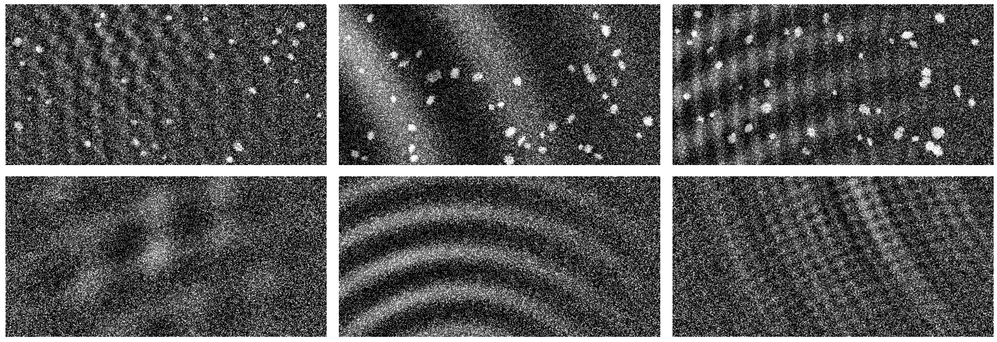
4.2.2. Synthetic Data Generation

In addition to the evaluation of the training approaches on natural data, we used a method to generate synthetic data to avoid the limiting characteristics of natural data in a separate evaluation. In this way, it is possible to generate any number of objects in an image and to ensure consistent annotations for each example. In contrast, manually generated annotations are always subject to errors, such as missing, inaccurate, or inconsistently marked regions.

To make a synthetic image ${\mathbf{I}}_j$ similar to the natural ones described in Section 4.2.1, we used a background of random noise by sampling values from a uniform distribution between 0 and $r_{\max }$ for each pixel and added a set of $n_j$ ellipses with intensities $k_{j,1},..,k_{j,n_j}$, centers at $p_{j,1},..,p_{j,n_j}$, rotations ${\phi }_{j,1},..,{\phi }_{j,n_j}$, and bounding box side lengths $(s_{j,1,x},s_{j,1,y}),..,(s_{j,n_j,x},s_{j,n_j,y})$ with $s_{\min }\le s_{j,u,v}\le s_{\max },1\le u\le n_j,v\in \{x,y\}$. The resulting images were overlaid with wave patterns to simulate image artifacts. For this purpose, we used a method presented in previous work [40] that creates a given number $w_j$ of sinus waves with center positions $c_{j,1}^{\left(\mathrm{w}\right)},..,c_{j,w_j}^{\left(\mathrm{w}\right)}$ and intensities $l_{j,1}^{\left(\mathrm{w}\right)},..,l_{j,w_j}^{\left(\mathrm{w}\right)}$. To create imperfections similar to those in natural images, the method uses an additional fading center point $c_{j,q}^{\left(\mathrm{f}\right)}$ and a fading rate ${\beta }_{j,q}$ for each wave q, which makes the wave intensity decrease with increasing distance to $c_{j,q}^{\left(\mathrm{f}\right)}$. This allows for different combinations of wave intensities to be visible at different positions. With a probability of $\gamma$, no waves were added to the image at all. Each parameter was randomly selected from a predefined interval, which is given in

Table 1. Parameter intervals for the generation of a synthetic image ${\mathbf{I}}_j$. The images produced with these parameters were scaled to a fixed interval after their generation.

Parameter	Interval	Description
$n_j$	$[0,50]$	number of ellipses
$r_{\max }$	$[1,1]$	noise intensity
$k_{j,i}$	$[0.5,1]$	ellipse intensity
$s_{j,u,v}$	$[6,18]$	bounding box side lengths
$l_{j,i}^{\left(\mathrm{w}\right)}$	$[0.75,1]$	wave intensity
$\gamma$	$[0.5,0.5]$	waves probability
$w_j$	$[0,5]$	number of waves
${\beta }_{j,q}$	$[0,1]$	wave fading rate

. Example images generated with this method are shown in Figure 6.

4.3. Results

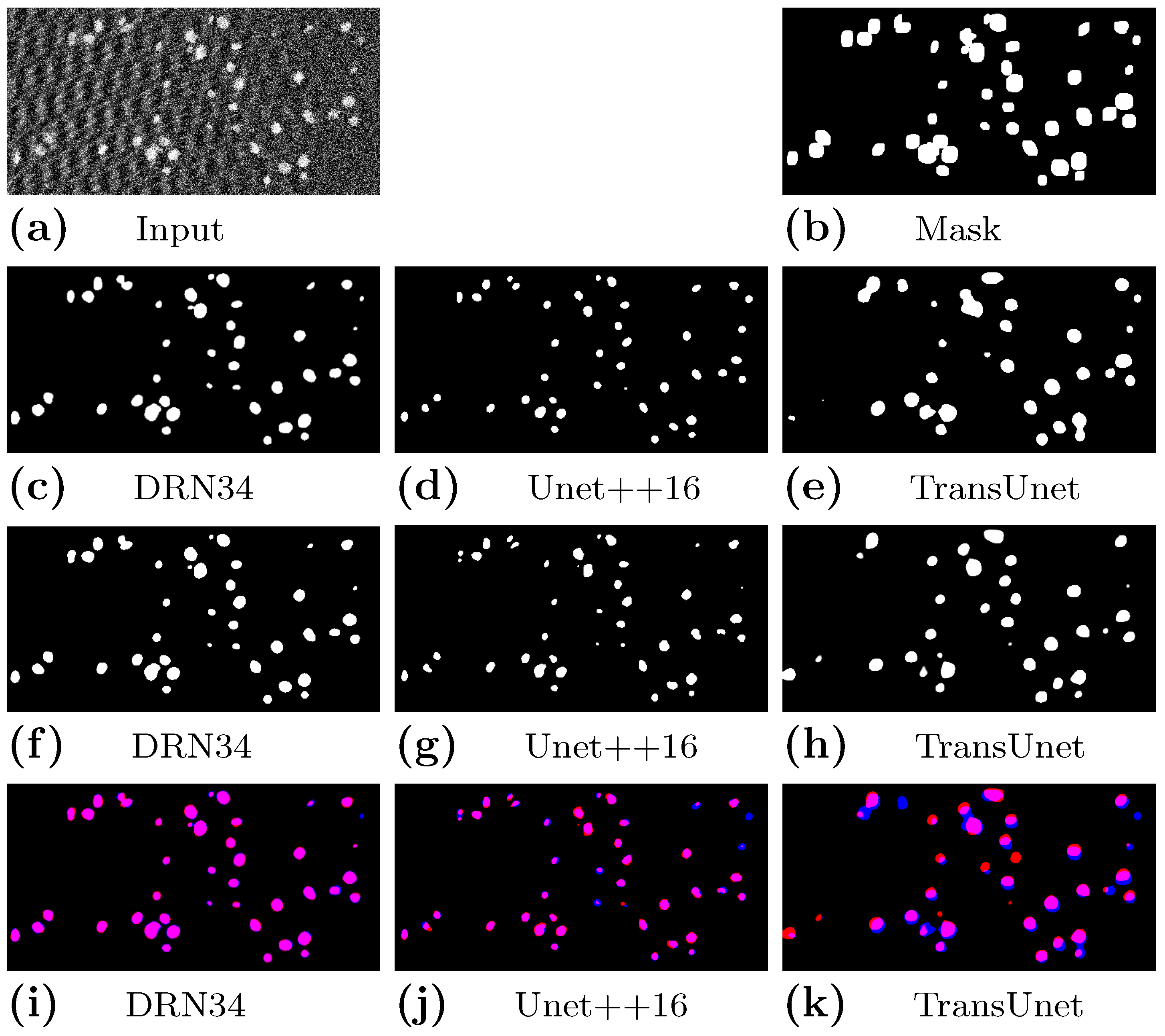
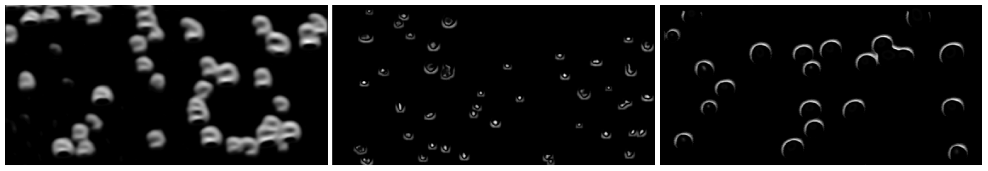
4.3.1. Results on Synthetic Images

When using synthetic data, each model was trained and evaluated on images with $512\times 256$ px, which are generated as described in Section 4.2.2. For the training, half of the images were generated without particles and the other half with a random number of objects between 1 and 50 from a uniform distribution. In the evaluation, we considered 1000 images with particles from the same generator. As we focused on the segmentation results, we omitted the case of 0 particles. Each training step and each evaluation step generated a new random example.

We used the results of the training with segmentation data as a reference for the achievable result quality since we expected a high level of training information to produce better results. The direct segmentation training (

Table 2. Results of a direct segmentation training on synthetic data followed by hard thresholding at 0.5 and connected components’ clustering.

Network	F1-Score	Recall	Precision
Dilated ResNet-18	0.989	0.999	0.981
Dilated ResNet-34	0.989	0.999	0.982
UNet++-8	0.986	0.995	0.980
UNet++-16	0.986	0.995	0.980
TransUNet	0.989	0.999	0.980

) reached F1-scores of greater than $98.0\%$ with all evaluated networks. It was noticeable that the different sizes of the same network architecture achieved the same F1-scores. Consequently, increasing the size of these architectures beyond their smaller versions did not seem to have a significant advantage for training a strongly supervised segmentation on the synthetic data. The CAM-based approach (

Table 3. Results of training counting networks with synthetic images followed by Score-CAM visualization, automatic thresholding, and connected components’ clustering.

Network	F1-Score	Recall	Precision
Dilated ResNet-18	0.978	0.967	0.992
Dilated ResNet-34	0.985	0.997	0.979
UNet++8	0.979	0.999	0.966
UNet++16	0.993	0.996	0.992
TransUNet	0.983	0.992	0.982

) showed slightly lower values in most cases, while one configuration, i.e., UNet++ with 16 start filters, even exceeded the value of its segmentation counterpart. The counting training combining the counting loss, the contrast loss, and the morphological loss (

Table 4. Results of training counting networks on synthetic images additionally employing the contrast loss (Section 3.3) and the morphological loss (Section 3.4). A following connected components’ clustering receives the output of the convolutional layer in the counting head after hard thresholding at 0.5.

Network	F1-Score	Recall	Precision
Dilated ResNet-18	0.945	0.903	0.996
Dilated ResNet-34	0.969	0.994	0.961
UNet++8	0.969	0.980	0.973
UNet++16	0.987	0.985	0.992
TransUNet	0.987	0.984	0.993

) showed F1-scores above $94.0\%$, which were, in most cases, slightly lower than those of the CAM-based approach.

Figure 7 shows example segmentations determined using the CAM-based method and the method based on the combination of the counting loss, the contrast loss, and the morphological loss.

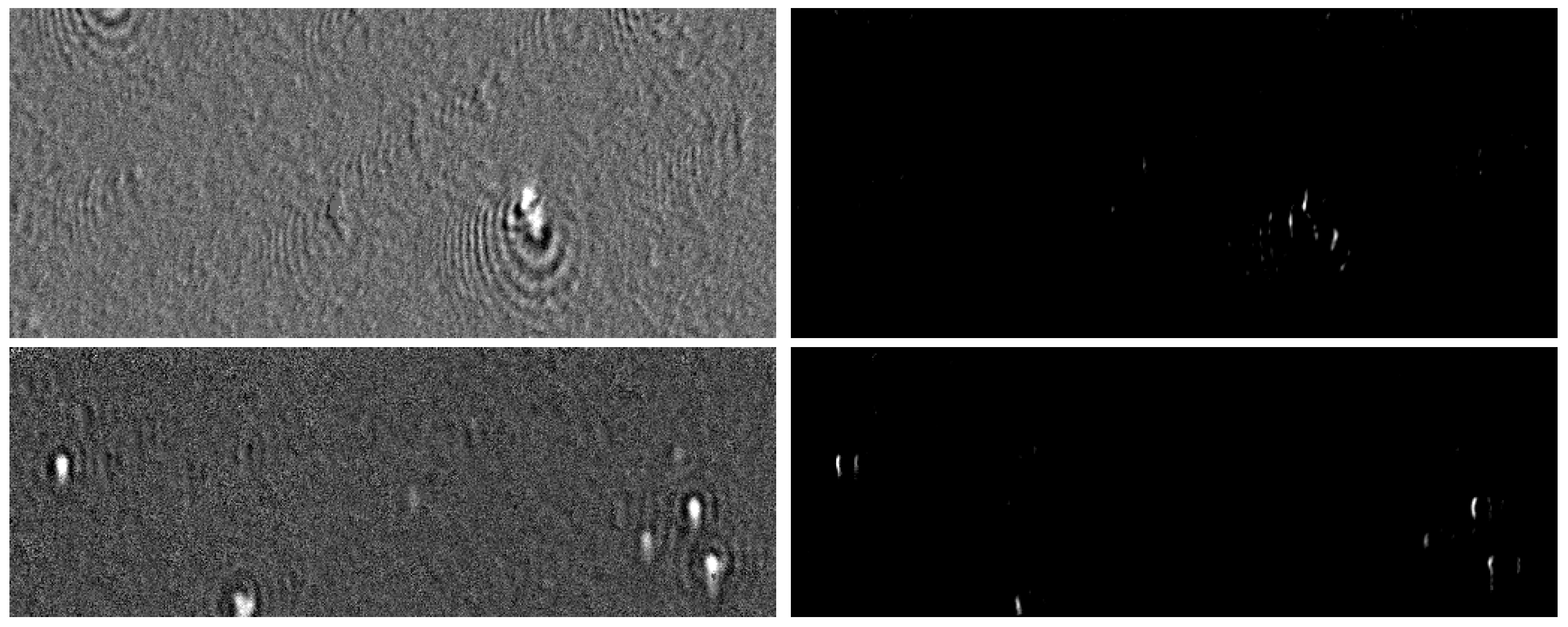
4.3.2. Results on Natural Images

We evaluated the training approaches on the natural data described in Section 4.2.1 using 11 datasets with and 18 datasets without objects of interest and selected $2/3$ (7, respectively 12) of the datasets for training and $1/3$ (4, respectively 6) for validation. In the training phase, only object counts at the image level were used. The datasets with particle occurrences consisted of a total of 11,133 images with a sum of 1909 particle trajectories, which provided a minimum of 0 and a maximum of 37 objects on an image. The particle-free datasets contained 22,572 images in total. In the end, we assessed the segmentation quality of all positive datasets using the segmented annotations. In each training step, we chose a random example from a random dataset, alternately using images with and without particles so that both cases occurred equally often. In the training, we extracted patches with a maximum side length of 512 px for each side. In the evaluation, we used the full images of the validation sets to compare the annotated segmentations with the implicitly learned ones. When using TransUNet, the patches that were cut out had to be padded with random noise for side lengths below 512 since this network only supports a constant image size given at construction time. The other networks can handle different input sizes directly.

Since our focus was on the usability of the presented learning approaches, we selected only datasets that showed comparatively low artifact intensities. In this way, we avoided effects that are caused by high-intensity artifacts and not by the training methods themselves. Despite this selection, image artifacts can never be completely prevented in real-world recordings. To deal with this, we applied an augmentation approach for increasing the robustness of a network against artifacts [40] that was also used in the creation of synthetic images (Section 4.2.2). It was applied randomly to the training samples with a probability of $50\%$ in each training step.

Unlike the synthetic data, the natural images have different sizes. The smallest images have a size of $450\times 170$ px and the largest $1692\times 400$ px. The reason is that, during the execution of the experiments in which the images were recorded, a free selection of the focal region took place by the person performing the experiments. Therefore, we used the full image sizes, which are different for each dataset, in the final evaluation.

For the analysis of the results with natural data, we additionally computed the F1-score on tracks as described in previous work [31]: a track is composed of detections from consecutive frames when the bounding boxes around these detections overlap significantly. We tolerated periods of up to three frames of missing detection before splitting a candidate track. After the construction, we discarded all tracks that appeared shorter than ten frames since we saw those occurrences as short-time disturbances based on the knowledge of typical track lengths. The track-related F1-score is a less-direct reflection of the segmentation results, but is an indicator of the usability in real-world applications, where short-term misdetections are filtered out in this way [31]. The overall values for the spatial and the tracking results were first averaged for each dataset individually and, then, combined by averaging these results so that the datasets with different numbers of images were weighted equally.

With segmentation based on highly supervised learning (

Table 5. Results of a direct segmentation training on natural data followed by hard thresholding at 0.5 and connected components’ clustering. For the evaluation with TransUNet, the images had to be split into patches and reassembled after segmentation because this network only supports a constant image size.

Network	Only Spatial			With Tracking
	F1-Score	Recall	Precision	F1 Score
Dilated ResNet-18	0.871	0.936	0.839	0.941
Dilated ResNet-34	0.870	0.893	0.873	0.914
UNet++-8	0.896	0.928	0.884	0.945
UNet++-16	0.890	0.894	0.909	0.941
TransUNet	0.873	0.947	0.828	0.929

), the spatial F1-scores were between $87.0\%$ and $89.6\%$. With track generation, i.e., filtering over time, a value of $94.5\%$ could be achieved. The counting training based purely on the counting loss failed to produce results above the single-digit percentage range. The reason for this lies in the combination of the learning methodology with the characteristics of the natural data and is detailed in Section 4.3.3. With the additional use of the contrast loss and the morphological loss, it was possible to reach values with spatial F1-scores between $81.7\%$ and $89.9\%$ and track-based F1-scores between $86.8\%$ and $95.5\%$, which are comparable to the results of the strongly supervised segmentation training. The detailed results for this method are listed in

Table 6. Results of training counting networks on natural images additionally employing the contrast loss (Section 3.3) and the morphological loss (Section 3.4). A following connected components’ clustering receives the output of the convolutional layer in the counting head after hard thresholding at 0.5. For the evaluation with TransUNet, the images had to be split into patches and reassembled after segmentation because this network only supports a constant image size.

Network	Only Spatial			With Tracking
	F1-Score	Recall	Precision	F1 Score
Dilated ResNet-18	0.879	0.925	0.854	0.937
Dilated ResNet-34	0.844	0.830	0.894	0.922
UNet++-8	0.899	0.929	0.890	0.955
UNet++-16	0.897	0.942	0.871	0.952
TransUNet	0.817	0.946	0.744	0.868

. An anomaly that could be observed for both types of training when using natural data was a slight degradation of the results when using the larger dilated ResNet and UNet++ variants compared to the smaller ones. This effect was not visible in the synthetic case. A possible explanation for this is the limited number of natural datasets. Since the image characteristics differed in each dataset, overfitting effects may occur with larger models.

Figure 8 shows example segmentations of the method based on the combination of the counting loss, contrast loss, and morphological loss.

4.3.3. Undesirable Effects

Unexpected shapes can occur in the segmentations extracted with the CAM-based method. Examples of shapes that occurred that way are shown in Figure 9. When training the same configuration multiple times, each new training may lead to different shapes marking the object for counting. The reason for that is a missing restriction since the counting loss can be satisfied by different shapes as long as they follow a consistent pattern within one trained model. The problem with this effect is that some shapes are hard to detect in downstream blob detection, so additional losses are necessary to ensure suitable features.

In the case of natural SPR image data, additional effects occurred. The examples in Figure 10 show two segmentations that were generated using the Score-CAM approach after being trained on a counting task. In both images, relevant regions are marked in an undesired way in which the object segmentations are distributed over the surrounding area. This is due to the fact that the objects in SPR images, i.e., particle signals, are naturally surrounded by wave patterns when they are made visible by the surface plasmon resonance effect. The waves around a particle, which may be stronger or weaker depending on the experimental setup, particle sizes, and materials are, therefore, sometimes detected as a feature to discover a particle signal. Although this identification as a relevant region for discovering a particle can make sense in the context of explainable AI, this result of the CAM-based segmentation is not suitable for downstream blob detection. Also, with specialized losses, it cannot be guaranteed that no undesirable effects occur when visualizing different sizes of the same segmented objects when the training is repeated. However, we were able to prevent scattered or open shapes by using the three combined losses.

5. Discussion

We presented a method for implicit segmentation training based on image-level annotations and compared it with a strongly supervised segmentation method. The evaluation was performed on three types of segmentation networks, two CNNs and one transformer-based network, on natural microscopy images, as well as synthetic data.

The strongly supervised segmentation training showed the most-stable results for the synthetic data: the F1-scores differed only slightly for the different network architectures, and there was no significant change in the F1-scores for the different sizes within one network architecture. When evaluated with natural data, the configurations achieved more-varying results in the purely spatial F1-scores, as well as the F1-scores based on the temporally linked tracks.

We evaluated a straightforward candidate for a solution using CAM to obtain segmentations from a counting network. In using a self-developed CAM-based approach, we showed that this methodology was able to achieve high F1-scores in certain cases, but was unsuitable when applied to natural data since it does not allow for controlling the extracted segmentation shapes. As a result, it may split a segmentation into fragments around the actual object when objects show unsharp edges. In the evaluated natural data, this effect was caused by local wave-like artifacts around objects. Even in the synthetic case, repeating the training can lead to undesirable shapes in the segmentation results, which cannot be controlled without modifying the underlying method. Therefore, we discourage its use beyond the scope of analyzing the reasons for a network output.

Training our weakly supervised approach based on additional losses, i.e., the contrast loss and the morphological loss, avoided undesired shapes by preferring high-contrast segmentations with blob-like structures. Despite an increased controllability of the segmentation results compared to the CAM-based approach, this type of training also led to more-divergent results than the strongly supervised approach when training multiple times with the same configuration. The size of a segmented object may vary with each training, as the morphological loss is only limited to blob-like shape characteristics, but not their exact sizes. If the determination of the exact sizes is of minor importance, this method can significantly reduce the time needed to generate annotations.

The presented morphological loss included more knowledge of the desired results than the counting loss and the contrast loss as it contained a vague expectation of the blob-like shape of objects and was, therefore, not suitable for all other use cases. Nevertheless, transferability to other application contexts where similar shapes are expected, e.g., other laboratory analyses such as fluorescence microscopy images, is expected.

To assess the transferability of the results, we also have to be aware of the data used. The synthetic examples offer a fixed data characteristic and an arbitrary number of objects and, by that, advantages that are usually not achievable in real applications. That means the results on these data showed a possibility rather than values that can be expected on natural data. For the feasibility check on natural data, a limited amount of datasets with rather low intensities of image artifacts was examined. Therefore, the findings cannot be considered generalizable without restrictions, but we expect that similar result characteristics can be found with other data and that improvements can be achieved with an increased amount and variety in the characteristics of the training data and optimized architectures.

6. Outlook

In this work, we implemented a straightforward extension to general segmentation networks. The explicit inclusion of operators tailored to blob-like structures could be used as an addition or alternative to supplementary loss functions to increase training stability. Thus, it is worth evaluating a combination of weakly supervised learning based on image-level counting with a segmentation structure optimized for the data characteristics at hand.

A possible extension of the losses could be an additional consideration of the separability of nearby or overlapping particles, as this aspect has not yet been considered.

An interesting question is whether the manual work of counting and noting the number of particles can be reduced further. This could be possible by using a binary classification of object presence in an image. This type of annotation can be created much faster. In the case of the microscopy data studied here, this step could be omitted completely in the case that a sufficient concentration of particles is used to ensure that objects are visible in each image. As examples without objects, samples completely without particles can be used. The risk in the case of images with multiple objects is that, for the classification of whether any objects are visible, not all objects have to be marked to decide whether objects are present at all. This could lead to missing detections, especially with increasing numbers of objects. It should be investigated whether a specialized network architecture can overcome this problem.

Extending the approach to include more-complex temporal information instead of a posterior linking of local object detection might be an additional way to improve the presented method.

References

1. Vădineanu, C.; Pelt, D.M.; Dzyubachyk, O.; Batenburg, K.J. An Analysis of the Impact of Annotation Errors on the Accuracy of Deep Learning for Cell Segmentation. In Proceedings of the 5th International Conference on Medical Imaging with Deep Learning, Zurich, Switzerland, 6–8 July 2022; Volume 172, pp. 1251–1267. [Google Scholar]
2. Zhang, D.; Han, J.; Cheng, G.; Yang, M. Weakly Supervised Object Localization and Detection: A Survey. IEEE Trans. Pattern Anal. Mach. Intell. 2022, 44, 5866–5885. [Google Scholar] [CrossRef]
3. Khan, M.A.; Menouar, H.; Hamila, R. Revisiting Crowd Counting: State-of-the-Art, Trends, and Future Perspectives. Image Vis. Comput. 2023, 129, 104597. [Google Scholar] [CrossRef]
4. Pandey, G.; Dukkipati, A. Learning to Segment with Image-Level Supervision. In Proceedings of the 2019 IEEE Winter Conference on Applications of Computer Vision (WACV), Waikoloa Village, HI, USA, 7–11 January 2019; pp. 1856–1865. [Google Scholar] [CrossRef]
5. Zhou, B.; Khosla, A.; Lapedriza, À.; Oliva, A.; Torralba, A. Learning Deep Features for Discriminative Localization. In Proceedings of the IEEE Conference on Computer Vision and Pattern Recognition, Boston, MA, USA, 7–12 June 2016; pp. 2921–2929. [Google Scholar]
6. Caicedo, J.C.; Roth, J.; Goodman, A.; Becker, T.; Karhohs, K.W.; Broisin, M.; Molnar, C.; McQuin, C.; Singh, S.; Theis, F.J.; et al. Evaluation of Deep Learning Strategies for Nucleus Segmentation in Fluorescence Images. Cytom. Part A 2019, 95, 952–965. [Google Scholar] [CrossRef]
7. Melanthota, S.K.; Gopal, D.; Chakrabarti, S.; Kashyap, A.A.; Radhakrishnan, R.; Mazumder, N. Deep Learning-Based Image Processing in Optical Microscopy. Biophys. Rev. 2022, 14, 463–481. [Google Scholar] [CrossRef]
8. Huo, Z.; Li, Y.; Chen, B.; Zhang, W.; Yang, X.; Yang, X. Recent Advances in Surface Plasmon Resonance Imaging and Biological Applications. Talanta 2023, 255, 124213. [Google Scholar] [CrossRef]
9. Hergenröder, R.; Weichert, F.; Wüstefeld, K.; Shpacovitch, V. 2.2 Virus Detection. In Volume 3 Applications; De Gruyter: Berlin, Germany; Boston, MA, USA, 2023; pp. 21–42. [Google Scholar] [CrossRef]
10. Libuschewski, P. Exploration of Cyber-Physical Systems for GPGPU Computer Vision-Based Detection of Biological Viruses. Ph.D. Thesis, TU Dortmund, Dortmund, Germany, 2017. [Google Scholar]
11. Oquab, M.; Bottou, L.; Laptev, I.; Sivic, J. Is Object Localization for Free?—Weakly-Supervised Learning with Convolutional Neural Networks. In Proceedings of the 2015 IEEE Conference on Computer Vision and Pattern Recognition (CVPR), Boston, MA, USA, 7–12 June 2015; pp. 685–694. [Google Scholar] [CrossRef]
12. Simonyan, K.; Zisserman, A. Very Deep Convolutional Networks for Large-Scale Image Recognition. arXiv 2015, arXiv:1409.1556. [Google Scholar]
13. Gao, G.; Gao, J.; Liu, Q.; Wang, Q.; Wang, Y. CNN-based Density Estimation and Crowd Counting: A Survey. arXiv 2020, arXiv:2003.12783. [Google Scholar]
14. Dosovitskiy, A.; Beyer, L.; Kolesnikov, A.; Weissenborn, D.; Zhai, X.; Unterthiner, T.; Dehghani, M.; Minderer, M.; Heigold, G.; Gelly, S.; et al. An Image is Worth 16 × 16 Words: Transformers for Image Recognition at Scale. arXiv 2020, arXiv:2010.11929. [Google Scholar]
15. Li, Y.; Zhang, X.; Chen, D. CSRNet: Dilated Convolutional Neural Networks for Understanding the Highly Congested Scenes. In Proceedings of the IEEE Conference on Computer Vision and Pattern Recognition, Salt Lake City, UT, USA, 18–23 June 2018; pp. 1091–1100. [Google Scholar] [CrossRef]
16. Liang, D.; Chen, X.; Xu, W.; Zhou, Y.; Bai, X. Transcrowd: Weakly-Supervised Crowd Counting With Transformers. Sci. China Inf. Sci. 2022, 65, 160104. [Google Scholar] [CrossRef]
17. Ronneberger, O.; Fischer, P.; Brox, T. U-Net: Convolutional Networks for Biomedical Image Segmentation. In Medical Image Computing and Computer-Assisted Intervention—MICCAI 2015, Proceedings of the 18th International Conference, Munich, Germany, 5–9 October 2015; Proceedings Part III 18; Springer: Berlin/Heidelberg, Germany, 2015; pp. 234–241. [Google Scholar]
18. Che, H.; Yin, X.X.; Sun, L.; Fu, Y.; Lu, R.; Zhang, Y. U-Net-Based Medical Image Segmentation. J. Healthc. Eng. 2022, 2022, 4189781. [Google Scholar] [CrossRef]
19. Zhou, Z.; Siddiquee, M.M.R.; Tajbakhsh, N.; Liang, J. UNet++: A Nested U-Net Architecture for Medical Image Segmentation. In Deep Learning in Medical Image Analysis and Multimodal Learning for Clinical Decision Support, Proceedings of the 4th International Workshop, DLMIA 2018, and 8th International Workshop, ML-CDS 2018, Held in Conjunction with MICCAI 2018, Granada, Spain, 20 September 2018; Proceedings 4; Springer: Berlin/Heidelberg, Germany, 2018; pp. 3–11. [Google Scholar]
20. Vaswani, A.; Shazeer, N.; Parmar, N.; Uszkoreit, J.; Jones, L.; Gomez, A.N.; Kaiser, L.; Polosukhin, I. Attention Is All You Need. Adv. Neural Inf. Process. Syst. 2017, 31, 6000–6010. [Google Scholar]
21. Gohel, P.; Singh, P.; Mohanty, M. Explainable AI: Current Status and Future Directions. arXiv 2021, arXiv:2107.07045. [Google Scholar]
22. Selvaraju, R.R.; Das, A.; Vedantam, R.; Cogswell, M.; Parikh, D.; Batra, D. Grad-CAM: Visual Explanations From Deep Networks via Gradient-Based Localization. In Proceedings of the IEEE International Conference on Computer Vision, Venice, Italy, 22–29 October 2017; pp. 618–626. [Google Scholar] [CrossRef]
23. Chattopadhyay, A.; Sarkar, A.; Howlader, P.; Balasubramanian, V.N. Grad-CAM++: Generalized Gradient-based Visual Explanations for Deep Convolutional Networks. In Proceedings of the 2018 IEEE Winter Conference on Applications of Computer Vision (WACV), Lake Tahoe, NV, USA, 12–15 March 2018; pp. 839–847. [Google Scholar] [CrossRef]
24. Srinivas, S.; Fleuret, F. Full-Gradient Representation for Neural Network Visualization. Adv. Neural Inf. Process. Syst. 2019, 33, 4124–4133. [Google Scholar]
25. Draelos, R.L.; Carin, L. Use HiResCAM Instead of Grad-CAM for Faithful Explanations of Convolutional Neural Networks. arXiv 2020, arXiv:2011.08891. [Google Scholar] [CrossRef]
26. Jiang, P.T.; Zhang, C.B.; Hou, Q.; Cheng, M.M.; Wei, Y. LayerCAM: Exploring Hierarchical Class Activation Maps for Localization. IEEE Trans. Image Process. 2021, 30, 5875–5888. [Google Scholar] [CrossRef]
27. Muhammad, M.B.; Yeasin, M. Eigen-CAM: Class Activation Map Using Principal Components. In Proceedings of the 2020 International Joint Conference on Neural Networks, Glasgow, UK, 29–24 July 2020; pp. 1–7. [Google Scholar] [CrossRef]
28. Desai, S.; Ramaswamy, H.G. Ablation-CAM: Visual Explanations for Deep Convolutional Network via Gradient-free Localization. In Proceedings of the 2020 IEEE Winter Conference on Applications of Computer Vision (WACV), Snowmass Village, CO, USA, 1–5 March 2020; pp. 972–980. [Google Scholar] [CrossRef]
29. Wang, H.; Du, M.; Yang, F.; Zhang, Z. Score-CAM: Improved Visual Explanations via Score-Weighted Class Activation Mapping. In Proceedings of the 2020 IEEE/CVF Conference on Computer Vision and Pattern Recognition (CVPR) Workshops, Seattle, WA, USA, 13–19 June 2020; pp. 24–25. [Google Scholar]
30. Zheng, H.; Yang, Z.; Liu, W.; Liang, J.; Li, Y. Improving Deep Neural Networks Using Softplus Units. In Proceedings of the 2015 International Joint Conference on Neural Networks (IJCNN), Killarney, Ireland, 12–17 July 2015; pp. 1–4. [Google Scholar] [CrossRef]
31. Wüstefeld, K.; Weichert, F. An Automated Rapid Test for Viral Nanoparticles Based on Spatiotemporal Deep Learning. In Proceedings of the 2020 IEEE Sensors Conference, Virtual, 25–28 October 2020; pp. 1–4. [Google Scholar] [CrossRef]
32. Pare, S.; Kumar, A.; Singh, G.K.; Bajaj, V. Image Segmentation Using Multilevel Thresholding: A Research Review. Iran. J. Sci. Technol. Trans. Electr. Eng. 2020, 44, 1–29. [Google Scholar] [CrossRef]
33. Paszke, A.; Gross, S.; Massa, F.; Lerer, A.; Bradbury, J.; Chanan, G.; Killeen, T.; Lin, Z.; Gimelshein, N.; Antiga, L.; et al. PyTorch: An Imperative Style, High-Performance Deep Learning Library. Adv. Neural Inf. Process. Syst. 2019, 33, 8026–8037. [Google Scholar]
34. Riba, E.; Mishkin, D.; Ponsa, D.; Rublee, E.; Bradski, G.R. Kornia: An Open Source Differentiable Computer Vision Library for PyTorch. In Proceedings of the 2020 IEEE Winter Conference on Applications of Computer Vision (WACV), Snowmass, CO, USA, 1–5 March 2020; pp. 3663–3672. [Google Scholar] [CrossRef]
35. Azad, R.; Aghdam, E.K.; Rauland, A.; Jia, Y.; Avval, A.H.; Bozorgpour, A.; Karimijafarbigloo, S.; Cohen, J.P.; Adeli, E.; Merhof, D. Medical Image Segmentation Review: The Success of U-Net. arXiv 2022, arXiv:2211.14830. [Google Scholar]
36. Chang, M.; Li, Q.; Feng, H.; Xu, Z. Spatial-Adaptive Network for Single Image Denoising. arXiv 2020, arXiv:2001.10291. [Google Scholar]
37. Wu, Y.; He, K. Group Normalization. In Proceedings of the European Conference on Computer Vision (ECCV), Munich, Germany, 8–14 September 2018; pp. 3–19. [Google Scholar] [CrossRef]
38. He, K.; Zhang, X.; Ren, S.; Sun, J. Deep Residual Learning for Image Recognition. arXiv 2015, arXiv:1512.03385. [Google Scholar]
39. Liang, A.; Liu, Q.; Wen, G.; Jiang, Z. The Surface-Plasmon-Resonance Effect of Nanogold/Silver and Its Analytical Applications. TrAC Trends Anal. Chem. 2012, 37, 32–47. [Google Scholar] [CrossRef]
40. Roth, A.; Wüstefeld, K.; Weichert, F. A Data-Centric Augmentation Approach for Disturbed Sensor Image Segmentation. J. Imaging 2021, 7, 206. [Google Scholar] [CrossRef] [PubMed]
Figure 1. Overview of the two approaches for learning segmentation indirectly through count training. The elements to the right of the vertical dashed line are only used in the evaluation when the left part has already been trained.
Applsci 13 12219 g001
Figure 2. Application of the counting head (blue) for image networks to enable the end-to-end counting of objects for segmentation networks. Normalization is achieved with the Z-score. The 1 × 1 convolution reduces the number of channels from an arbitrary number m to 1. The learned positive factor multiplication multiplies the input number with a weight that is guaranteed to be positive by the prior use of a 1 × 1 convolution followed by a Softplus activation [30]. The input and output are contained in gray boxes, and the actual segmentation part is in black boxes.
Applsci 13 12219 g002
Figure 3. Scheme of the training setup of a counting network with the contrast loss (Section 3.3) and the morphological loss (Section 3.4) as additional losses between the implicit segmentation and the explicit counting.
Applsci 13 12219 g003
Figure 4. A dilated residual block, as used in the dilated ResNets of this work. The k × k notation specifies the kernel size. The parameters d 1 = 1 , d 2 = 2 , and d 3 = 4 give the dilation. The number of channels is given as c. GN denotes a group normalization [37] with a group size of 8. The last convolution uses a dilation value of 1.
Applsci 13 12219 g004
Figure 5. Examples of surface plasmon resonance effect (SPR) [39] images recorded with the plasmon-assisted microscopy of nano-objects (PAMONO) sensor [9]. All images contain artifacts of rather low intensities. The upper row shows signals from 1, 3, and 7 annotated particles (from left to right), which can be seen as bright spots of different intensities. Around some of the particles, typical SPR wave patterns are visible. The lower row shows images without particles.
Applsci 13 12219 g005
Figure 6. Examples of synthetically generated images. The images in the upper row contain elliptical objects of different sizes, circularities, and intensities on a random noise background overlaid with random waves. The images in the lower row were generated in the same way, but contain no objects.
Applsci 13 12219 g006
Figure 7. Example input (a), the mask of generated objects (b), segmentations created using the CAM-based approach (ce), and the approach using the counting loss, the contrast loss, and the morphological loss (fh). In the overlayed images (ik), the results of the CAM-based approach are represented with blue pixels, and the results of the loss-based approach are marked red. Pixels where positive segmentation values were generated for both approaches are shown in purple.
Applsci 13 12219 g007
Figure 8. Example input (a), the mask of manually annotated objects (b), and segmentations created using the loss-based approach with different network architectures (ce). The output determined on the basis of TransUNet had to be divided into patches due to the specification of a constant input size in combination with different image sizes in the test data. Because of this, abrupt changes can be seen at the borders of these sections due to object areas that have been split. A noticeable feature in the results is that two individual objects are combined in one area in the annotation mask (second marker from the right). Only the dilated ResNet (DRN34) separated the two objects correctly.
Applsci 13 12219 g008
Figure 9. Unexpected shapes in the segmentation results of three synthetic example images. The segmentations were extracted with Score-CAM after training only using the counting loss.
Applsci 13 12219 g009
Figure 10. Undesired shapes in the segmentation results of two natural example images. The networks were trained only using the counting loss. The segmentations were generated using the Score-CAM approach.
Applsci 13 12219 g010