Time-Frequency Analysis and Neural Networks for Detecting Short-Circuited Turns in Transformers in Both Transient and Steady-State Regimes Using Vibration Signals

Abstract

Transformers are vital elements in electrical networks, but they are prone to various faults throughout their service life. Among these, a winding short-circuit fault is of particular concern to researchers, as it is a crucial and vulnerable component of the transformers. Therefore, if this fault is not addressed at an early stage, it can increase costs for users and affect industrial processes as well as other electrical machines. In recent years, the analysis of vibration signals has emerged as one of the most promising solutions for detecting faults in transformers. Nonetheless, it is not a straightforward process because of the nonstationary properties of the vibration signals and their high-level noise, as well as their different features when the transformer operates under different conditions. Based on the previously mentioned points, the motivation of this work is to contribute a methodology that can detect different severities of short-circuited turns (SCTs) in transformers in both transient and steady-state operating regimes using vibration signals. The proposed approach consists of a wavelet-based denoising stage, a short-time Fourier transform (STFT)-based analysis stage for the transient state, a Fourier transform (FT)-based analysis stage for the steady-state, the application of two fault indicators, i.e., the energy index and the total harmonic distortion index, and two neural networks for automatic diagnosis. To evaluate the effectiveness of the proposed methodology, a modified transformer is used to experimentally reproduce different levels of SCTs, i.e., 0-healthy, 5, 10, 15, 20, 25, and 30 SCTs, in a controlled way. The obtained results show that the proposed approach can detect the fault condition, starting from an initial stage for consolidation and a severe stage to accurately assess the fault severity, achieving accuracy values of 90%.

1. Introduction

The development of monitoring systems for assessing the health condition of electrical machines has played a significant role in the industry [1]. In particular, transformers are crucial elements in electrical energy networks, allowing for the distribution and transmission of electrical energy and providing proper power for numerous applications [2]. Although they are robust machines, they will eventually suffer from failures produced mainly by electrical and mechanical stresses that act on them during their operation [3]. Among the diverse faults that can arise in a transformer, faults in the windings (FW), representing about 50% of all failures in a transformer [4], have received special interest from researchers because these elements are the most important and vulnerable in transformers. Therefore, if this fault is not addressed early, it can increase costs for users and affect industrial processes. In addition, it can damage other elements of the transformer, and depending on the number of elements damaged, a failure in the transmission line and damage to other transformers can be generated. For these reasons, different methods such as frequency response analysis, leakage reactance measurement, short-circuit impedance measurement, dissolved gas analysis, voltage–current locus diagram, and vibration analysis (VA) have been proposed for monitoring the transformer condition, with VA being an efficient and reliable noninvasive method for detecting faults in the windings of transformers [5]. Nevertheless, its efficacy mainly depends on the identification or estimation of suitable features that exist in vibration signals [6]. Hence, a method or technique capable of extracting suitable features from vibration signals is of significant importance for early fault detection in transformers under different operating conditions.

During the last few years, numerous signal processing techniques for fault detection in transformers using vibration signals have been introduced, namely, the Fourier transform (FT) and its variations such as the short-time Fourier transform (STFT), which are the most popular signal processing techniques for monitoring the condition of transformers [7,8,9]. In general, FT-based methods are useful for identifying or estimating the frequencies contained in a signal, which can be associated with a damage condition; however, their results can be compromised depending on the quantity of analyzed data, noise in the signal, leakage (i.e., creation of non-existent spectral components), and transient characteristics or phenomena found in the signal [10,11]. As an alternative to the problems found in the FT-based methods, recent works propose the use of other advanced signal processing methods. Babaei and M. Moradi [12] use the wavelet transform (WT) for differentiating internal faults from magnetizing inrush currents in the presence of current transformer saturation. In [13], the empirical WT is used by Zhao and Xu to detect winding deformations. Lu et al. [14] combine the use of an improved empirical WT and extreme machine learning technique to diagnose various fault transformer conditions. DC bias in power transformers is detected by using the wavelet packet energy distribution [15]. Other WT variations, i.e., the probabilistic WT, are presented by Seo et al. [16] for the partial discharge measurement of a transformer. On the other hand, in recent years, the use of decomposition methods has also been explored [17,18,19,20,21]. A comparison between the empirical mode decomposition (EMD) method, the ensemble EMD (EEMD) method, and the complete EEMD (CEEMD) to diagnose short circuit faults is presented by Mejia et al. [18]. An extension of the CEEMD, namely, CEEMD with adaptive noise (CEEMDAN), is presented in [19] to detect winding and core loosening. In addition, the variational mode decomposition (VMD) is used by Hong et al. [20] to assess the degradation of transformer windings. Finally, the nonlinear mode decomposition method is present by Huerta et al. [21] to diagnose SCTs. Although promising results have been reported with these techniques, some issues still need to be taken into account. For instance, it can be highlighted that the WT is a method designated to decompose nonstationary signals (i.e., signals with changing characteristics) into a set of frequency bands; however, its good results depend mainly on the proper choice of both the decomposition level and the mother wavelet [22]. On the other hand, the HHT, which combines the empirical mode decomposition with the Hilbert transform, is an adaptive method capable of estimating the instantaneous frequencies contained in a signal, but it suffers from a phenomenon called mode mixing (i.e., waves with different frequency are assigned to the same mode or frequency band) [23], which can limit the correct monitoring of the transformer condition.

From the methods reviewed above, it is evident that each of them can have certain advantages or disadvantages in specific scenarios. In this regard, it is of great importance to select, combine, modify, and consequently leverage their advantages in order to develop a more efficient method in terms of processing time and complexity, as well as applicability. For instance, FT-based methods have significant advantages such as a low computation burden and do not require meticulous calibration [24]; on the other hand, STFT or WT-based methods can handle nonstationary signals, as in the case of vibration signals in transformers, particularly when the vibrations generated during the starting transient are considered [21]. Similarly, the capabilities of the WT can be utilized to reduce the inherent noise in the vibration signals. This task is particularly challenging when the noise needs to be removed from both transient and steady-state signals without compromising the frequency information necessary for the diagnosis.

Therefore, in the search of a more efficient and robust method for the detection of short-circuited turns (SCTs) in transformers, it is essential that the employed method can promptly identify the damage in both transient and steady state operating regimes, thus expanding its applicability across of a wider range of transformer applications. With this goal in mind, this paper contributes the adroit integration of a new method that combines different signal processing techniques to effectively detect and quantify the severity of SCTs in transformers in both regimes of operation, providing a more comprehensive and accurate diagnosis method. In general, the method combines the WT for signal denoising, STFT for transient analysis, FT for steady-state analysis, the application of a comb filter to remove harmonic components during the transient regimen, two nonlinear measurements, i.e., energy (ENE) and total harmonic distortion (THD), for characterizing the damage severity, and two neural networks for the automatic diagnosis of SCTs under both regimes of operation using vibration signals. To evaluate the effectiveness of the proposed method, a modified transformer and its triaxial vibration signals under various operating conditions (i.e., 0-healthy, 5, 10, 15, 20, 25, 30, and 35 SCTs) are analyzed, considering both transient and steady states. The results demonstrate that the proposed method can accurately detect and characterize the damage severity in both regimes with a high degree of accuracy.

The remaining of the paper is as follows. Section 2 describes the theoretical background of the proposed methodology. The proposed methodology and the experimental setup to test it are described in Section 3. Section 4 shows the obtained results and general discussions. Finally, conclusions are drawn in Section 5.

2. Theoretical Background

This section provides a brief theoretical background about the main topics used in this work.

2.1. Vibrations in Transformers

Vibration signals have a direct correlation with the mechanical and electrical performance of transformers [4,20]. These vibrations are predominantly generated within the transformer core and windings during its operation. Core vibrations are manly induced by the magnetostriction phenomenon, which describes the dimensional changes in ferromagnetic materials when exposed to magnetic fields [25,26]. The fundamental vibration frequency in the core is twice the input power system frequency, and higher harmonics emerge due to the nonlinearity of the magnetostriction phenomenon. The vibration amplitude, a_core, is directly proportional to the square of the voltage, U, as follows [26]:

$$a_{core}\alpha U^2$$

(1)

The forces resulting from the vibrations caused by magnetostriction manifest in a perpendicular direction to the core [25]. On the other hand, winding vibrations, which have axial and radial components, result from electromagnetic forces acting on the windings due to the interaction between the leakage flux density and the current in the windings. Assuming the current is nearly sinusoidal, the primary harmonic, a_winding, of winding vibrations is directly proportional to the square of the current, I, as follows [26]:

$$a_{winding}\alpha I^2$$

(2)

As vibration signals are correlated with the mechanical and electrical performance of the transformer core and windings, a damage condition in the winding, e.g., a SCT condition, will change their frequency content, leaving the opportunity to develop methodologies based on signal processing techniques which can characterize such frequency changes. However, this task is not a straightforward process due to the high-level noise and nonstationary nature of the vibration signals.

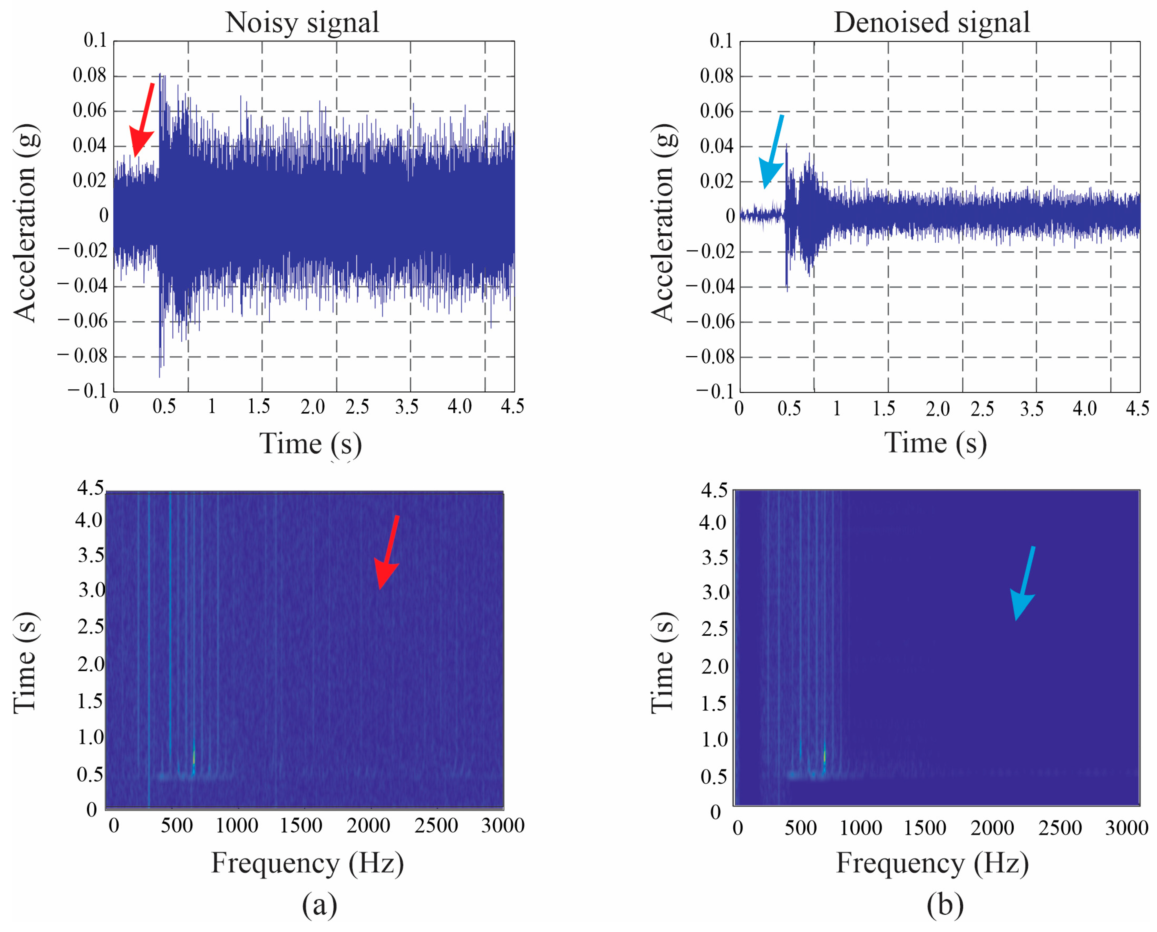
2.2. Wavelet Denoising

Vibration signals are frequently affected by diverse sources and levels of noise, which can significantly hinder the extraction of useful information from the signal. Among the various denoising techniques, wavelet-based denoising has demonstrated excellent performance in various applications [27,28,29,30] due to (i) its inherent capability to handle both stationary and nonstationary signals and (ii) its bank filter-based computation. The steps that describe this process are as follows:

• Introduce a noisy signal into the process. A noisy signal is described as follows [27]:

  $$s_i=f+\sigma e_i$$

  (3)

  where $f$ is the original signal, $e_i$ is a Gaussian white noise, and $\sigma$ is the noise level.
• In the next step, the noisy signal is decomposed using the discrete WT (DWT). This method allows for the decomposition of the signal into sets of coefficients at different frequency levels according to the following [30]:

  $$\begin{array}{c}DWT\left[n, a^j\right]={\displaystyle \sum _{m=0}^{N-1}}x\left[m\right]{\psi }_j^{*}\left[m-n\right]\\ {\psi }_j\left[n\right]=\frac{1}{\sqrt{a^j}}\psi \left(\frac{n}{a^j}\right)\end{array}$$

  (4)

  where x[m] is the original discretized signal, ψ is the discretized mother wavelet, a is a scaling parameter, n is the shift parameter that determines the location of the wavelet, and the parameter j is the decomposition level.
• To eliminate the noise at each decomposition level, a threshold value is necessary. There are different threshold estimators, e.g., rigrsure, sqtwolog, hearsure, and minimaxi. Once the threshold estimator has been selected, either hard or soft thresholding can be applied [27,28,29,30].
• Finally, the inverse DWT is used to reconstruct the denoised signal using the newly thresholded coefficients. Further details can be found in [27,28,29,30].

Once the noise has been removed from the signal, useful frequency information can be extracted more effectively.

2.3. Short-Time Fourier Transform

FT is a mathematical operation that converts a time-domain signal into a frequency-domain signal, providing information about the frequencies present in the original signal [31]. When dealing with nonstationary signals, the STFT is the preferred choice, as it produces a time–frequency representation. In essence, the STFT consists of segmenting the input signal and applying the FT to each segment as follows [31]:

$$X\left(m, \omega \right)=\sum _{n=-\infty }^{\infty }x\left[n\right]\omega \left[n-m\right]e^{-j\omega n}$$

(5)

where $\omega$ is a window function, n and m are indices for the samples in the signal, and $e^{-j\omega n}$ is the transformation kernel.

The length of the time window defines the trade-off between time and frequency resolution, while its shape can impact the issue of leakage due to the windowing of finite data sets [31,32]. Further details can be found in [32].

2.4. Measurement Functions

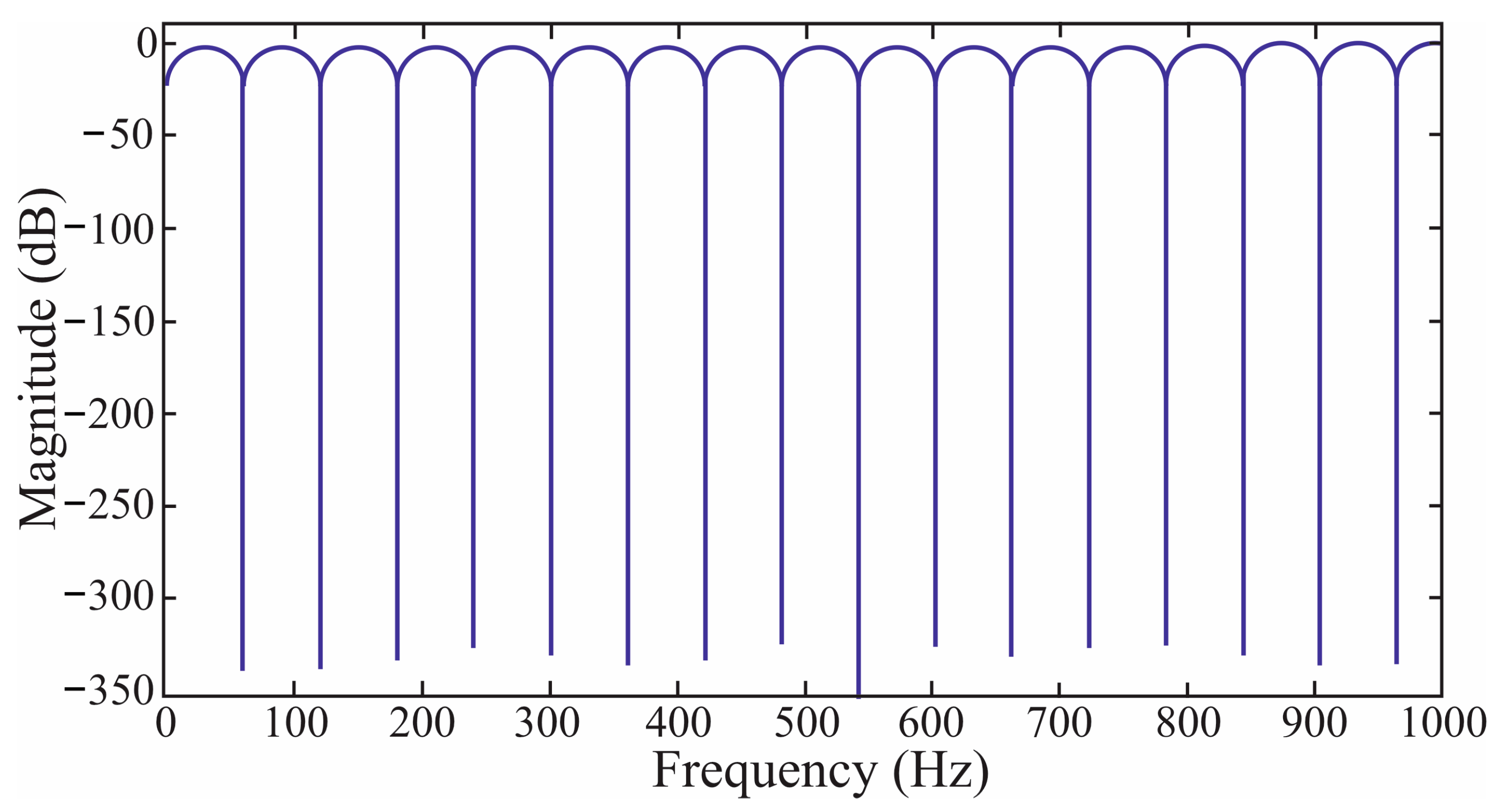
To characterize the frequency content of the vibration signal in both regimes, namely, transient and steady states, it is divided into two parts, one for each regimen. For their characterization, two indicators, i.e., energy (ENE) and total harmonic distortion (THD), have been selected. The ENE index is used for the transient state because it can serve as a representative measure of the time-varying amplitudes of each frequency component in their time–frequency representation. On the other hand, the THD index is used for the steady state because it can represent how much the harmonic content can change relative to the fundamental frequency component. It is important to note that, in both cases, it is expected that the frequency content changes in the presence of a SCT condition. The proposed indices are calculated as follows [33]:

$$THD=\frac{E_{Harmonics}}{E_{f_0}}$$

(6)

$$ENE=\sum _{f=0}^{f_s/2}{\left[X\left|f\right|\right]}^2$$

(7)

where $E_{Harmonics}$ is the energy related to the harmonic components, $E_{f_0}$ is the energy related to the main frequency, X[f] is the signal in the frequency domain, and fs is the sampling frequency.

2.5. Comb Filter

To remove the stationary frequency components from a transient signal, a comb filter can be used. A feed-forward comb filter (FFCF) involves the addition or subtraction of a delayed version of the original signal. The discrete output, y, of an FFCF when x is used as the input signal is defined as follows [34]:

$$y\left[k\right]=\left(x\left[k\right]+\alpha x\left[k-N\right]\right)/2$$

(8)

where N is the number of delay samples of the input signal and $\alpha$ is a scaling factor that satisfies $\left|\alpha \right|\le 1$. The frequency response of the FFCF exhibits a periodic sequence of notches and peaks. The peaks reach their maximum amplitude when $\alpha \pm 1$. The notches are centered at frequencies $f_c$ defined as follows [34]:

$$f_c\left(r\right)=\left(F_{s}r\right)/N$$

(9)

where $F_s$ is the sampling frequency of the signal and r takes the values 0, 1, 2, …, N/2. The frequency response of an FFCF can be observed in Figure 1.

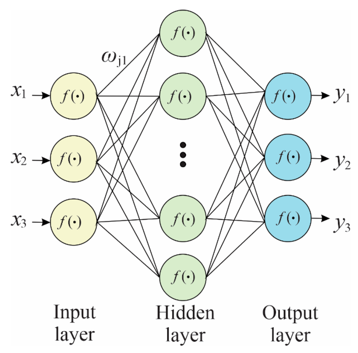
2.6. Artificial Neural Networks

For automatic pattern recognition, different machine learning models can be used. Among them, artificial neural networks (ANNs) are one of the most popular and simple models [35]. ANNs are inspired by the functioning of the human brain. These networks consist of interconnected neurons organized into layers, namely, the input layer, hidden layers, and the output layer, as shown in Figure 2. Each neuron receives a set of weighted inputs which are multiplied by their respective weights and summed. Subsequently, a nonlinear activation function, such as log-sigmoid, tan-sigmoid, and linear transfer functions, is applied to this weighted sum to determine the neuron’s output. Information flows from the input layer through one or more hidden layers before reaching the output layer. Backpropagation is used to train the network, adjusting the weights so that the output approximates the desired output. Here, different training algorithms such as Levenberg–Marquardt, scaled conjugate gradient, and variable learning rate backpropagation, among others, can be used. In each algorithm, different settings such as the number of epochs, minimum error, and type of performance measurement, among others, can be selected. Further details can be reviewed in [35].

The mathematical formulation for a single neuron is as follows:

$$y=f\left(\sum _{i=1}^I{\omega }_i{x}_i+b\right)$$

(10)

where y, ω_i, x_i, b, f(·), and I are the output, weights, inputs, bias, activation function, and total number of inputs, respectively.

In order to evaluate the performance of the ANNs, various metrics, namely, accuracy, recall, specificity, precision, and F1-score, can be used. Their mathematical formulation for binary classes is as follows:

$$accuracy=\frac{TP+TN}{TP+TN+FP+FN}$$

(11)

$$recall=\frac{TP}{TP+FN}$$

(12)

$$specificity=\frac{TN}{TN+FP}$$

(13)

$$precision=\frac{TP}{TP+FP}$$

(14)

$$F1\_score=\frac{2TP}{2TP+FP+FN}$$

(15)

where TP, TN, FP, and FN represent true positives, true negatives, false positives, and false negatives, respectively. In general, accuracy represents the proportion of overall correct predictions. Recall indicates the proportion of true positive cases correctly identified, while specificity represents the proportion of true negative cases correctly identified. Precision measures the proportion of correct positive predictions, and F1_score is a metric that provides a balance between precision and recall, being useful when there are class imbalances. Each metric addresses a specific aspect of the model’s performance, allowing for a more comprehensive and detailed evaluation.

3. Methodology and Experimental Setup

3.1. Proposed Methodology

The proposed methodology to diagnose different levels of severity of short-circuit faults in a transformer under transient and steady state regimes of operation through the analysis of vibration signals is shown in Figure 3. In general, this proposal is based on the adroit integration of several methods that effectively addresses the needs of this application, e.g., noise rejection, removal of harmonic oscillation components during transformer energization, appropriate selection and use of fault indicators to characterize the fault severity, and low-complex but efficient pattern recognition algorithms for automatic classification. In this regard, the proposed methodology consists of the following stages:

Stage 1—Noise reduction in the vibration signals. According to Section 2.2, a wavelet denoising stage is developed, removing frequencies with amplitude fluctuation that are not related to the fault condition and, consequently, highlighting the frequency components which can provide useful information for the diagnosis. After extensive experimentation, it was determined that a Daubechies 45 (db45) mother wavelet, a decomposition level of 7, the threshold estimator, sqtwolog, and soft thresholding provide satisfactory results in the denoising task.

Stage 2—Removal of stationary frequency components from a transient signal. Once the noise has been removed, the clean vibration signals are analyzed in both transient and steady states. It is important to remark that this work presents a methodology to diagnose SCTs faults in both regimes, allowing the condition monitoring and fault detection in a wider range of transformer applications. For the transient signals, the comb filter presented in Section 2.5 is first applied in order to remove the stationary frequency components, i.e., integer multiples of 60 Hz. This process allows the analysis of the transient regimen without affecting the harmonic changes and their duration.

Stage 3—Time–frequency and frequency-domain analysis. For the transient signal, its time–frequency representation is obtained through the STFT. In this case, with the elimination of stationary frequency components in stage 2, the frequency components related to the energization transient of the transformer are only retained. On the other hand, in the case of the steady-state signals, the frequency components of the vibration signals are obtained using the FT. This regimen is considered stationary since the parameters of the harmonic components remain constant. In this stage, the mathematical formulation of Section 2.3 is used.

Stage 4—Index calculation. Due to the nature of the two types of analysis (transient and stable), two different indices are proposed. For the case of transient state, the ENE index is used and, for the case of steady state, the THD index is calculated according to Equations (6) and (7).

Stage 5—Classification and diagnosis. Finally, once the indices have been obtained for each transformer operating condition (transient state regimen and steady state regimen), two independent ANNs are designed and trained to perform the automatic transformer diagnosis. The metrics used to evaluate the performance of the ANNs are presented in Section 2.6 and their settings are presented in Section 4.4.

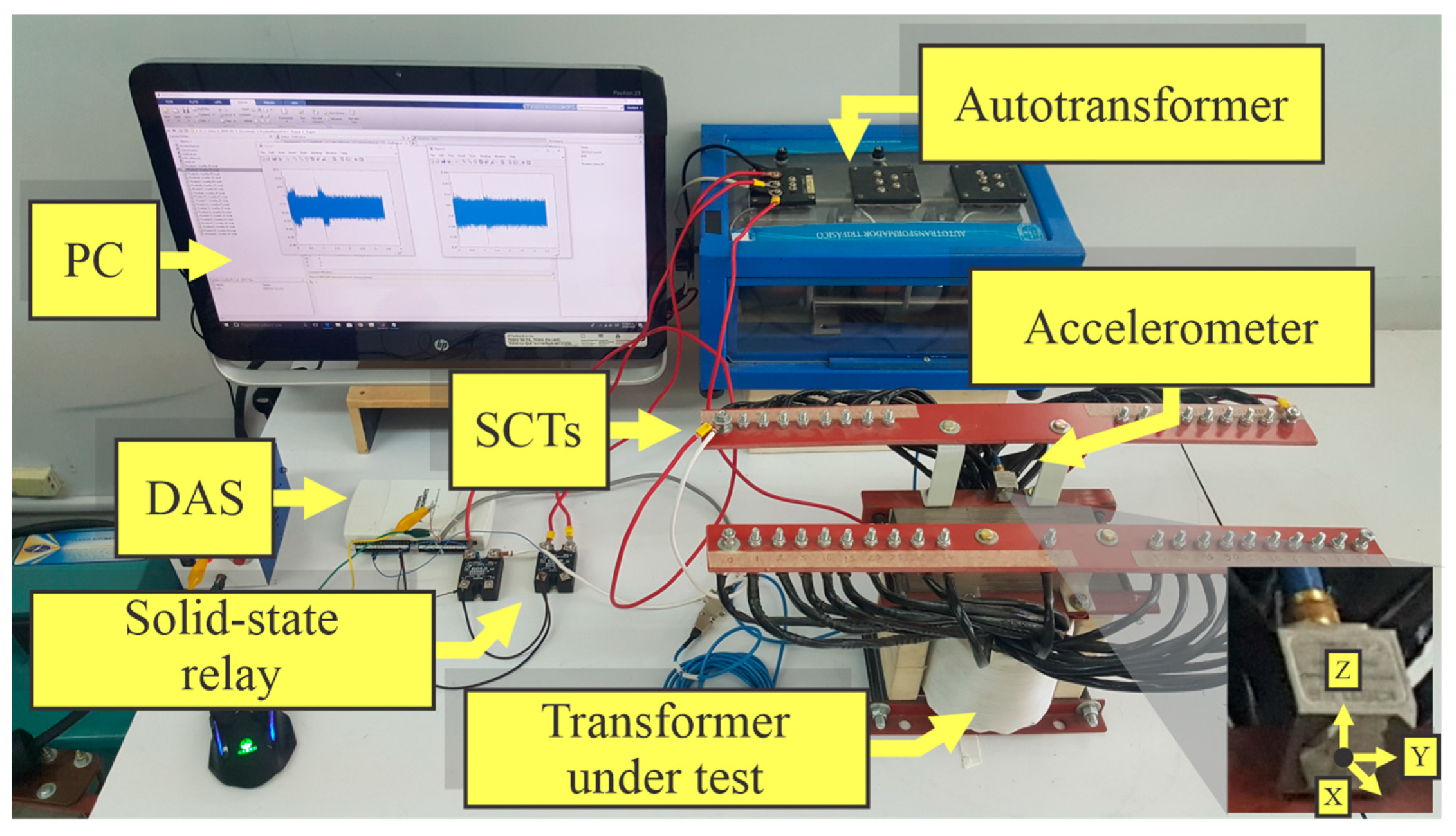
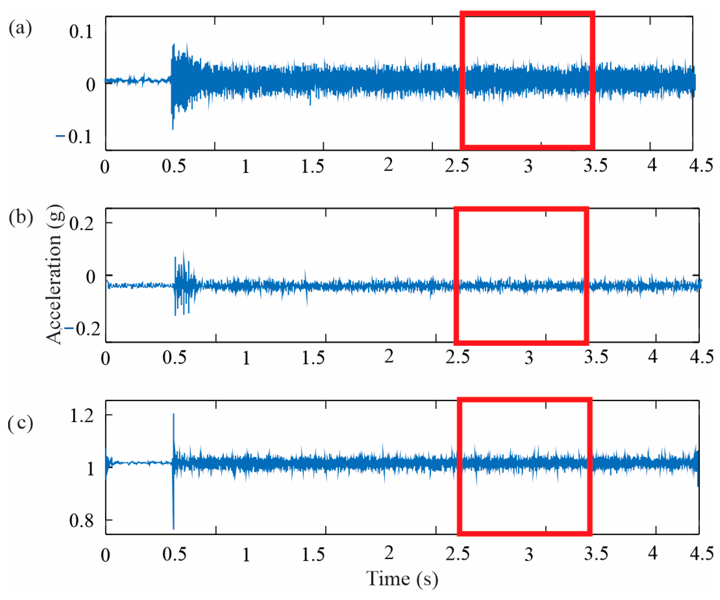
3.2. Experimentation

The experimental setup, shown in Figure 4, consists of a single-phase transformer with a rating of 1.5 kVA, operating at 120 V, and equipped with a winding of 135 turns. This transformer is modified to artificially generate eight different conditions of SCTs (i.e., 0-healthy, 5, 10, 15, 20, 25, 30, and 35 SCTs). Each condition is measured 100 times, resulting in a database of 2400 tests, where each test contains the vibrations for the trees’ axes (Vx, Vy, and Vz). The vibration signals are captured using a triaxial accelerometer model 8395A from KISTLER, which is located on the clamping frame of the transformer. The accelerometer has a measurement range of 10 g, with a resolution of 400 mV/g and a bandwidth from 0 to 1000 Hz. The vibration signals are acquired by a 16-bit analog-to-digital converter (ADC) within the data acquisition system (DAS) of the National Instruments NI-USB 6211 board. The sampling frequency is set to 6000 samples per second, and the vibrations signals are sampled for a duration of 4.5 s, ensuring the acquisition of both transient and steady-state data. This results in 27,000 samples for each test. An example of the triaxial vibration signals obtained are shown in Figure 5. A solid-state relay model SAP4050D is used to activate the transformer, which remains unconnected to any load during the diagnosis process. An autotransformer is used to de-energize the transformer after each test. The transient state occurs when the vibrations are produced by the magnetostriction phenomenon induced by the inrush current in the transformer. After a visual examination, the data window from 0.5 s to 1.5 s is determined to be the energizing transient, followed by 3 s which correspond to the steady-state operation. The signal from 0 s to 0.5 s corresponds to the de-energized transformer. Finally, a personal computer(PC) running Matlab v2018 software is used to implement the overall methodology.

4. Experimentation and Results

4.1. Wavelet Denoising

According to the methodology depicted in Figure 3, the first step involves the application of the wavelet denoising stage. Figure 6 illustrates the performance of the denoising stage. In Figure 6a, the noisy signal is shown in both the time domain and its time–frequency representation. As observed, the background noise (i.e., the existing noise when the transformer in not connected) from 0 to 0.5 s exhibits a considerable amplitude, which is also evident across the time–frequency plane (see the red arrows). Conversely, in Figure 6b, the background noise has been substantially removed (see the blue arrows), demonstrating the effectiveness of the proposed denoising stage.

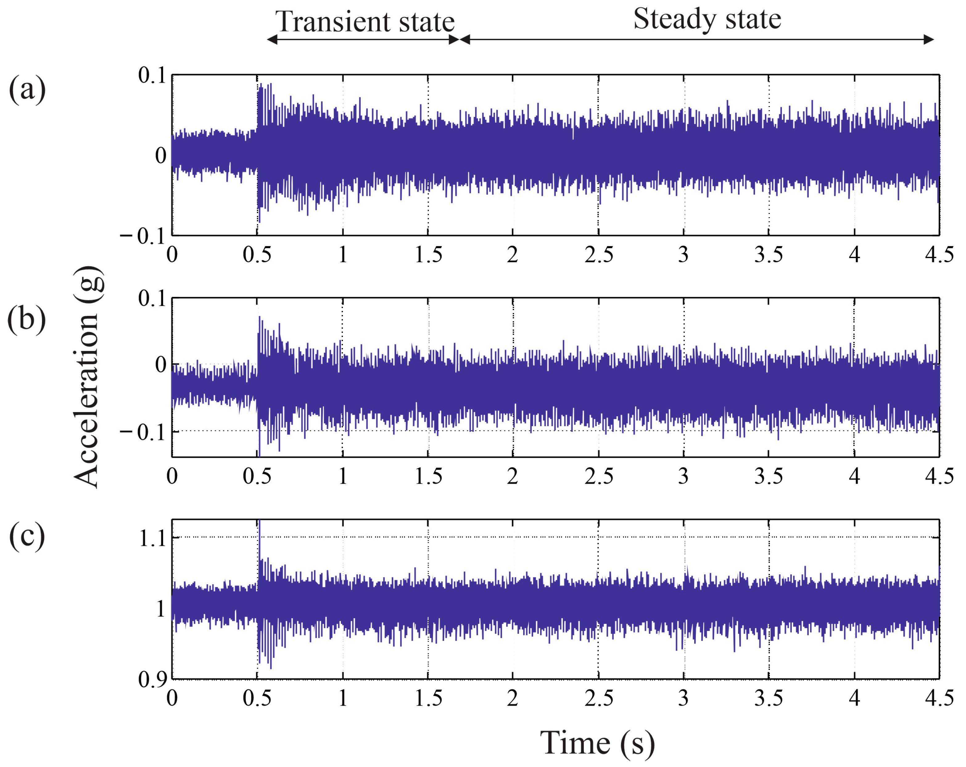
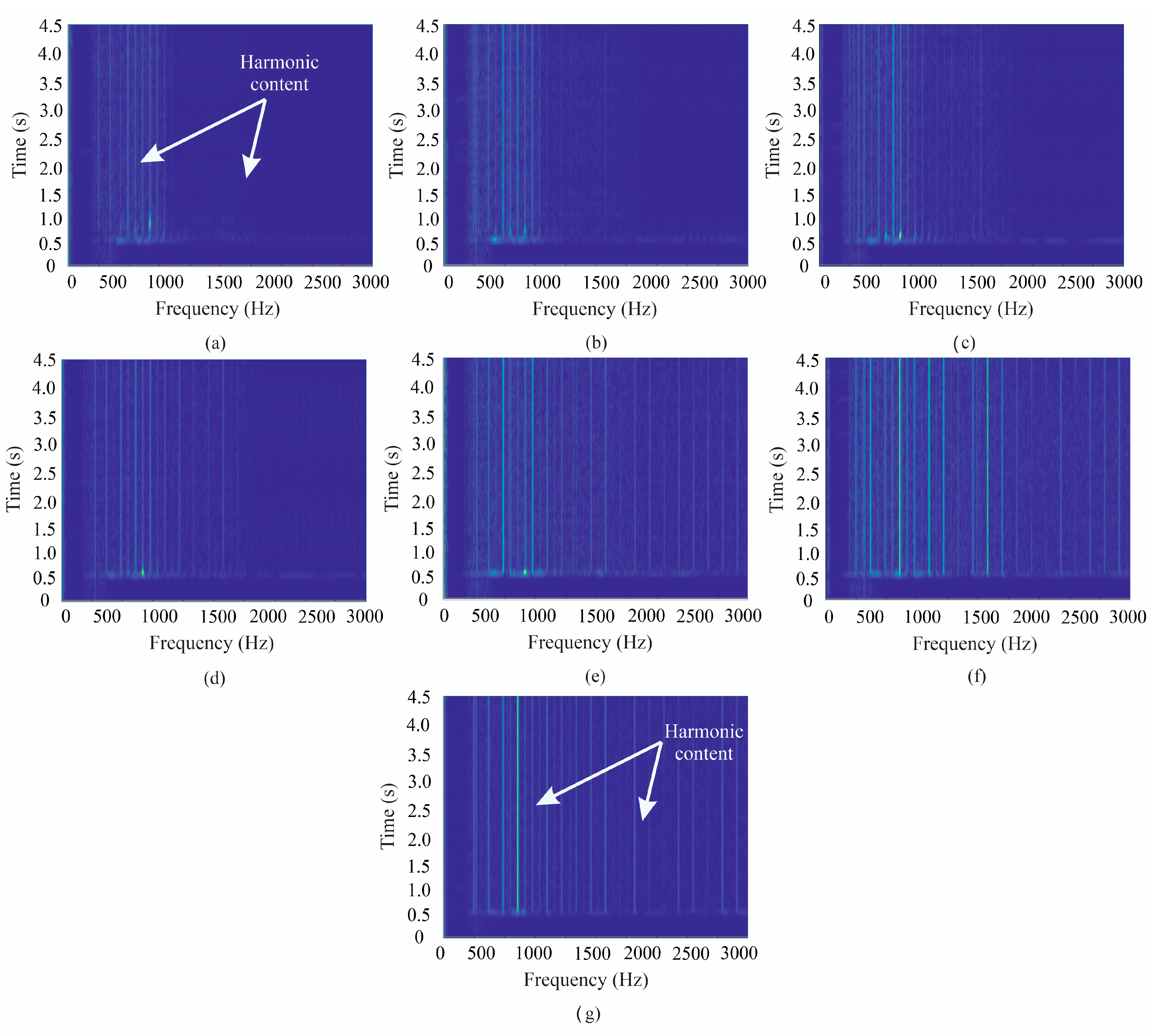
4.2. Results for the Transient State

Once the noise of the vibration signal has been reduced, the comb filter is applied to eliminate the harmonic content of the signal; therefore, only the frequency components that emerge during the transformer energization are retained, facilitating the diagnosis of SCT conditions in the transformer during this regimen.

Figure 7 and Figure 8 display the time–frequency representations of the vibration signals for each SCT condition, both without and with the comb filter, respectively. In Figure 7, it is evident that the harmonic content increases throughout the time–frequency plane relative to the fault severity, being somehow lower in Figure 7a (0 SCTs) and higher in Figure 7g (30 SCTs). It is worth noting that the straight lines which are observed in the time–frequency plane represent constant frequency components (i.e., harmonic components); although the magnitudes of these components are indicated by a color scale, their specific values are not taken into account in this work since they are quantified in a global manner by the proposed indices. On the other hand, as can be seen, most of the stationary content has been removed (see Figure 8), leaving only the transient components, as depicted by the white arrows. It is also observed that the transient frequency content increases relative to the fault severity, being somehow lower in Figure 8a (0 SCTs) and higher in Figure 8g (30 SCTs). In order to characterize the impact of the SCTs on the vibration signals during the transformer energization, the ENE index is computed according to Equation (7). In general, the ENE index can be interpreted as the sum of all the nonzero frequency components present in the time–frequency plane.

Figure 9 shows the boxplot results for the ENE index in all of the transformer conditions. Each boxplot summarizes the results for the 100 tests of each SCT condition. Each subfigure corresponds to one axis (Vx, Vy, and Vz). In order to have the same reference in the three axes, the values are normalized, with the 0 SCTs condition serving as the baseline, resulting in an index value of 1 for that condition. This approach can be useful for establishing a reference in different transformers. In Figure 9, it is observed that the ENE index increases in accordance with the severity of damage in the three vibration axes (see the red arrows), making it a valuable feature for fault severity detection. From a visual inspection, the results for the X-axis exhibit a more proportional trend relative to the fault severity. For a more quantitative understanding,

Table 1. Average ENE values for the different SCTs conditions.

SCTs
Signal	0	5	10	15	20	25	30
Vx	1	1.0787	1.1394	1.3116	1.3564	1.8395	2.7043
Vy	1	0.9002	1.2071	1.2624	1.2409	1.8031	1.8108
Vz	1	1.0071	1.0095	1.0291	1.0341	1.0795	1.0709

presents the average values of the ENE index for each axis.

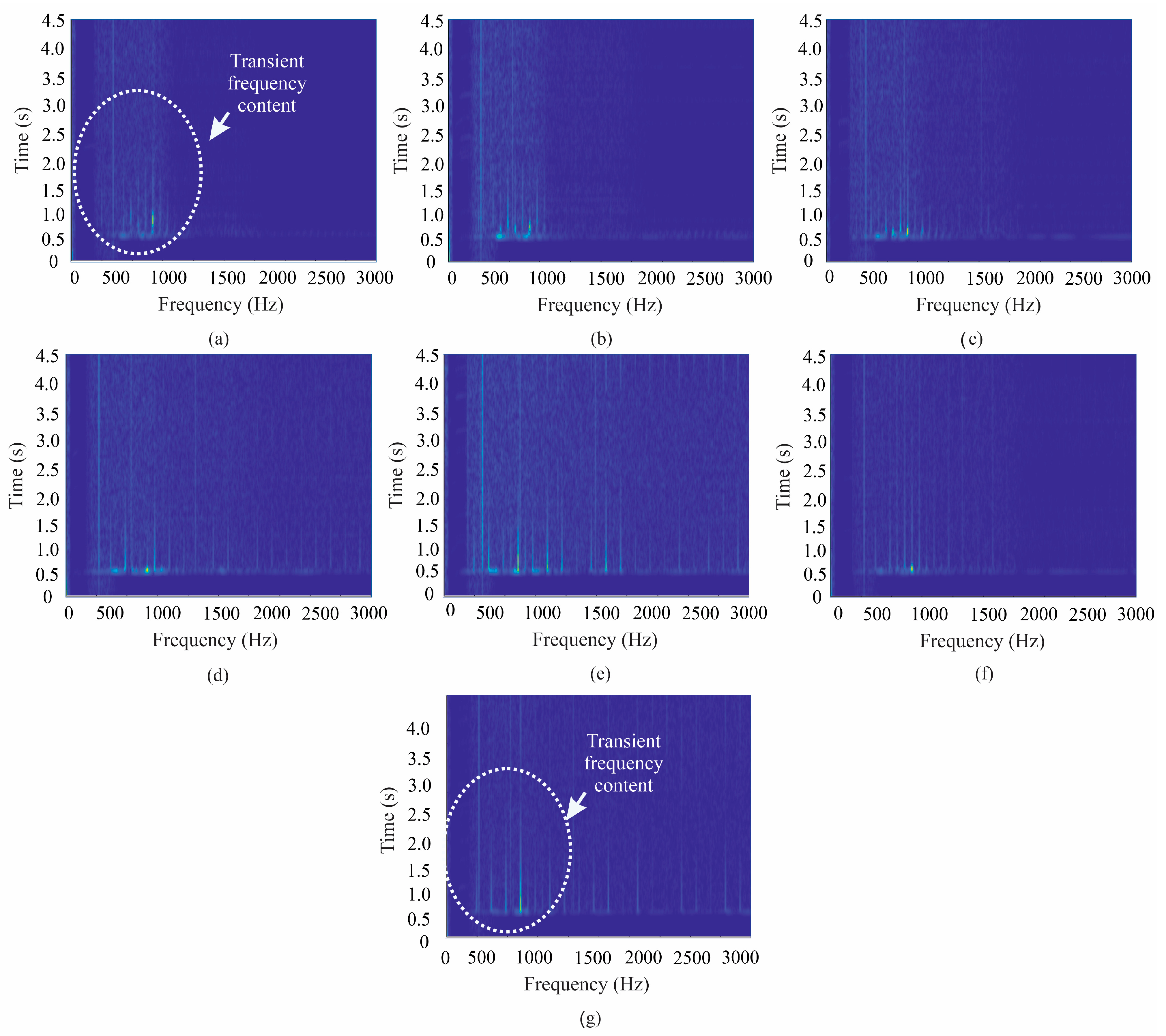
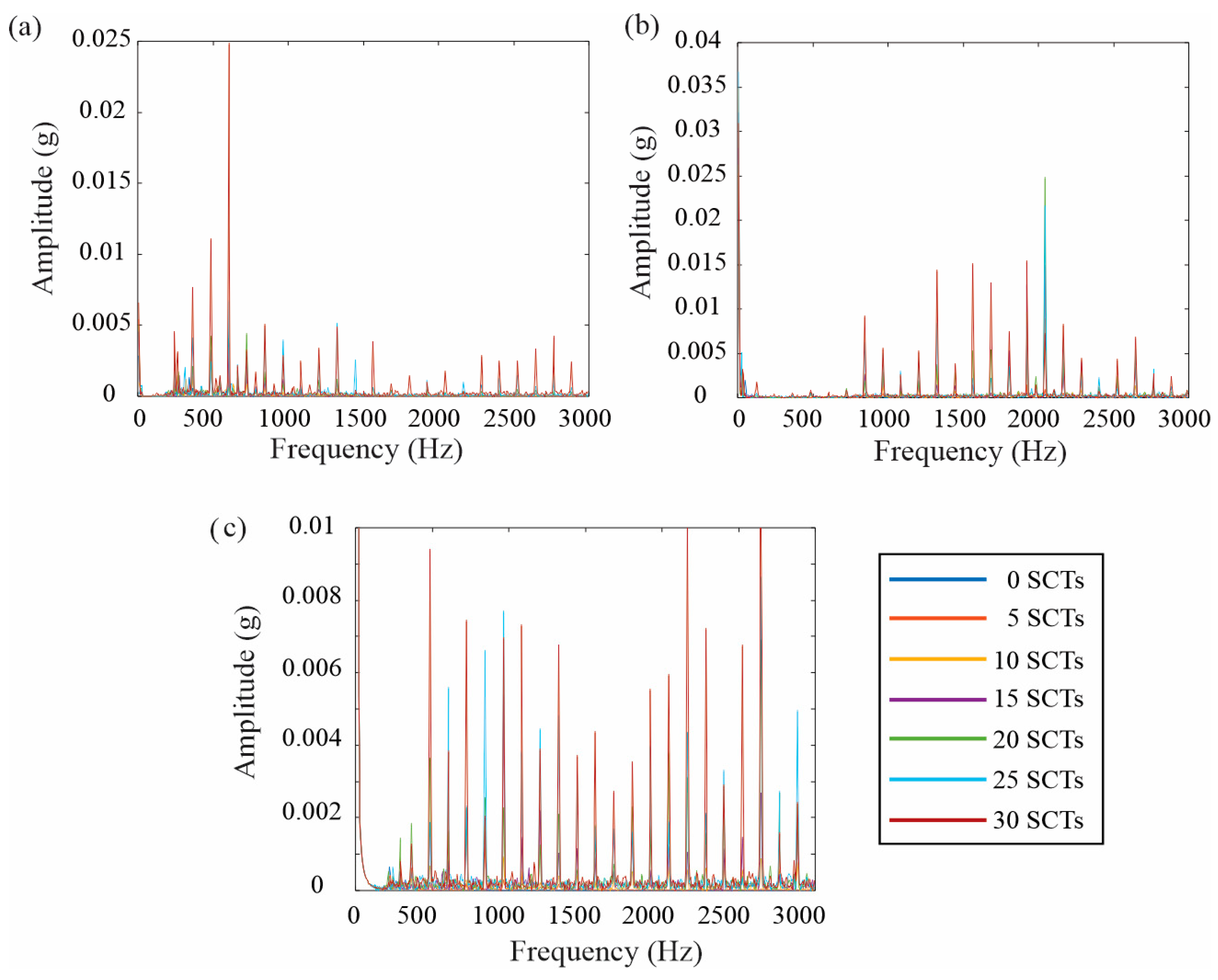
4.3. Results for the Steady State

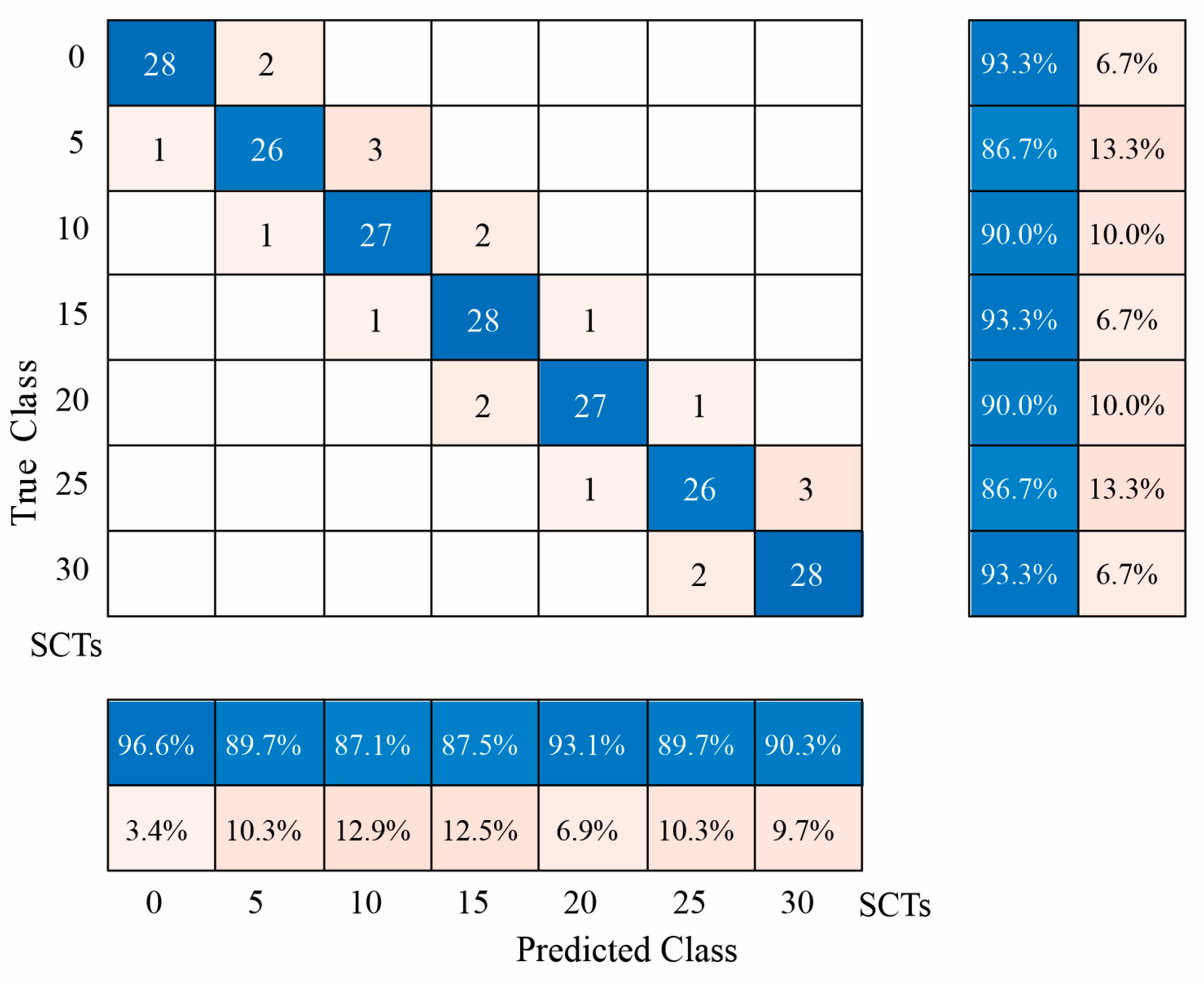
For diagnosing the SCT fault in steady state, a segment of the vibration signal during the steady state is extracted. In Figure 10, the red rectangle depicts the selected signal. Once the signal has been selected, the FT with a Gaussian window, applied to minimize the leakage problem, is used to obtain its spectrum. Figure 11 shows the resulting spectra for all of the SCTs conditions in the three axes (Vx, Vy, and Vz). As can be observed, there are different changes in the frequency components for each SCT condition. At this point, it is not important to visually distinguish among spectra since they will be differentiated through a quantitative index. In order to do so, the THD index, following Equation (6), is used. Figure 12 shows the normalized THD values, with each boxplot summarizing the results from 100 tests for each SCT condition. Each subfigure corresponds to one axis (Vx, Vy, and Vz). Similar to the ENE index, the values are also normalized, with the 0 SCTs condition serving as the baseline, leading to an index value of 1 for that condition. This strategy can be helpful for establishing a reference in different transformers. In Figure 12, it is observed that the THD index can also increase in accordance with the severity of damage in the three vibration axes (see the red arrows). From a visual inspection, the results for both the X-axis and the X-axis exhibit proportional trends relative to the fault severity; however, the trend of the Z-axis appears more consistent, as indicated by the narrower boxplots.

Table 2. Average THD values for the different SCTs conditions.

SCTs
Signal	0	5	10	15	20	25	30
Vx	1	1.1750	1.2670	1.5372	1.8855	2.5642	2.7475
Vy	1	1.0455	1.8513	2.4707	2.5634	2.6960	3.3665
Vz	1	1.0228	1.7007	3.1712	3.9219	5.1645	6.0375

presents the average values of the THD index for each axis.

4.4. ANN Results

From the trends and patterns of both indices, ENE and THD, shown in Figure 9 and Figure 12, it becomes evident that the application of a machine learning model for automatic fault severity diagnosis is feasible. As mentioned in Section 2.6, in this work, the ANN model is selected. After conducting thorough experiments aimed at achieving satisfactory classification results, the resulting NN architecture comprises three inputs (i.e., the index value of each vibration axis), twelve neurons in the hidden layer, and seven outputs, i.e., one for each SCT condition. This architecture follows the one presented in Figure 2. The training algorithm used is the scaled conjugate gradient. The total data were divided in 70% for training and 30% for validation. It is worth noting that two separate ANNs, each with the aforementioned structure, are used for each operating regime, as outlined in the proposed methodology in Figure 3. Figure 13 and Figure 14 present the obtained confusion matrices, where accuracy total values of 90% are obtained.

Table 3. Metrics for the values shown in Figure 13.

SCT Class	Accuracy	Recall	Specificity	Precision	F1-Score
0	0.9000	0.9000	0.9889	0.9310	0.9153
5	0.8333	0.8333	0.9778	0.8621	0.8475
10	0.9333	0.9333	0.9833	0.9032	0.9180
15	0.8333	0.8333	0.9778	0.8621	0.8475
20	0.9000	0.9000	0.9667	0.8182	0.8571
25	0.9333	0.9333	0.9944	0.9655	0.9492
30	0.9667	0.9667	0.9944	0.9667	0.9667

and

Table 4. Metrics for the values shown in Figure 14.

SCT Class	Accuracy	Recall	Specificity	Precision	F1-Score
0	0.9333	0.9333	0.9944	0.9655	0.9492
5	0.8667	0.8667	0.9833	0.8966	0.8814
10	0.9000	0.9000	0.9778	0.8710	0.8852
15	0.9333	0.9333	0.9778	0.8750	0.9032
20	0.9000	0.9000	0.9889	0.9310	0.9153
25	0.8667	0.8667	0.9833	0.8966	0.8814
30	0.9333	0.9333	0.9833	0.9032	0.9180

show the accuracy, recall, specificity, precision, and F1-score metrics for the confusion matrices shown in Figure 13 and Figure 14, respectively. These values are computed using the mathematical formulations of Section 2.6 by taking the values of one against all. As can be observed, most of the values are higher than 0.9 (90%), indicating the good performance of the proposed ANN models under different metrics. However, it is also evident that some signals are more difficult to accurately classify in terms of precision, e.g., 15 and 20 SCT classes in the transient state (Table 3). These values will be the reference during the development and application of new and more efficient machine learning-based models in terms of complexity and accuracy.

Also, a k-fold cross validation with k = 3 is carried out in order to avoid possible biased results due to the random split of data [36,37]. The obtained accuracy values are 90.1% (transient state) and 90.4% (steady state), showing highly similar results and, consequently, the reliability of the proposed ANN models. Although promising results have been obtained, there is still an opportunity to further research other machine learning-based models.

4.5. Discussions

Detecting winding faults in transformers, mainly at an early stage (i.e., low severity), from vibration signals represents a significant challenge due to their nonstationary properties and high-level noise inherent in vibrations. This challenge is more difficult when the transformer that generates them operates in transient regimens. Therefore, there is a pressing need to introduce innovative methods or approaches, such as the one outlined in this study, which can accurately evaluate the transformer’s condition when faced with these scenarios. In this regard,

Table 5. Comparison of the proposed methodology against other relevant methodologies that use vibration signals for winding faults in transformers.

Reference	Signal Processing Methods	Analyzed State	Number of Sensors Employed	Detected Faults	Severity Levels	Automatic Diagnosis
Proposal	Wavelet denoising and FT-based methods	Transient and steady	1	SCTs	6	ANNs
[3]	Electromagnetic force analysis	Steady	5	Winding loosening	3	--
[13]	Empirical wavelet transform and HT	Transient and steady	2	Winding deformation	3	--
[19]	CEEMDAN and multiscale dispersion entropy	Steady	1	Winding and core loosening	1	Density peaks clustering
[20]	VMD and WT	Steady	1	Winding deformation	3	CNN
[21]	NMD and HT-based RMS	Transient and steady	1	SCTs	6	FLS

presents a comparative analysis between the proposed approach and the most recent methodologies documented in the literature for detecting the presence of failures in the winding of a transformer from vibration signals. Specifically, it details the techniques or methods employed in each approach, the assessed transformer operating state, the severity levels, and the pattern recognition algorithm used for automatic diagnosis.

As shown in Table 5, unlike other works that have focused on only one operating state [3,19,20], this proposal presents a solution for two operating regimes (i.e., transient and steady), which is desirable in order to provide a solution for a wider range of transformer applications. It is also important to mention that the proposed method provides a complete solution for condition monitoring since an automatic pattern recognition for automatic classification is included, eliminating the need for an expert to interpret the monitored data, which could be the case for the works presented in [3,13]. Finally, while similar results are found in [21] and in this work, it is crucial to emphasize that the NMD method involves much more complex and time-consuming signal processing compared to the methods used in this work. This condition makes the proposal a more promising solution for software/hardware-based online monitoring implementations, mainly if low-end processors are used.

Although the proposed research has yielded good results, it is important to describe diverse limitations, which should be investigated in future research: (1) the proposal must be tested during diverse types of linear and nonlinear loads, as the present study is focused exclusively on an unloaded transformer and (2) the methodology robustness must be explored under other fault conditions, i.e., winding deformations and core faults, among others, including their combination, since in real practice, the appearance of multiple combined faults is normal.

5. Conclusions

Vibration analysis for fault detection in transformers is one of the most employed methods. In this work, a novel methodology for diagnosing SCTs in transformers in both operating regimes (i.e., transient and steady state) by using vibration signals is proposed. This approach is experimentally validated using a modified transformer subjected to various levels of fault severity (i.e., 0-healthy, 5, 10, 15, 20, 25, and 30 SCTs), resulting in accuracy average values of 90% in both operating conditions. For the transient state, a minimum value of 81.8% (20 SCTs) and a maximum of 96.7% (30 SCTs) are obtained; on the contrary, for the steady state, these values correspond to a minimum of 87.1% (10 SCTs) and a maximum of 96.6% (0 SCTs).

Despite the inherent properties of vibration signals, i.e., high-level noise and nonstationary properties, the adroit integration or various signal processing stages in the proposed method allows for several advantages. The noise rejection stage effectively reduces components that are not of interest and mitigates negative effects during the estimation of harmonic components using STFT and FT. Furthermore, this proposal does not necessitate complex time–frequency kernels or techniques, since the proposed approach allows the resolution limitations of STFT to be disregarded due to the energy conservation (Parseval’s theorem) and the use of the ENE and THD indices, which are calculated based on the energy parameters of the signal. Additionally, the comb filter facilitates the removal of steady state components, enabling a focused analysis on transient components related to faults.

The ENE and THD indices, combined with the proposed signal processing techniques (i.e., wavelet denoising, comb filter-based filtering, and Fourier-based transformations), have proven to be effective indicators of fault severity, as their values somehow increase with the severity of the fault. This suggests their potential applicability to other transformers.

In future work, the detection of SCTs in the transformer operating with linear and nonlinear loads will be explored. Additionally, more sophisticated machine learning and deep learning-based models will be researched to further enhance the accuracy of the diagnosis.

References

1. Khalili Senobari, R.; Sadeh, J.; Borsi, H. Frequency response analysis (FRA) of transformers as a tool for fault detection and location: A review. Electr. Power Syst. Res. 2018, 155, 172–183. [Google Scholar] [CrossRef]
2. Barkas, D.; Chronis, I.; Psomopoulos, C. Failure mapping and critical measurements for the operating condition assessment of power transformers. Energy Rep. 2022, 8, 527–547. [Google Scholar] [CrossRef]
3. Zhou, H.; Hong, K.; Huang, H.; Zhou, J. Transformer winding fault detection by vibration analysis methods. Appl. Acoust. 2016, 114, 136–146. [Google Scholar] [CrossRef]
4. Zheng, J.; Huang, H.; Pan, J. Detection of Winding Faults Based on a Characterization of the Nonlinear Dynamics of Transformers. IEEE Trans. Instrum. Meas. 2018, 68, 206–214. [Google Scholar] [CrossRef]
5. Bagheri, M.; Zollanvari, A.; Nezhivenko, S. Transformer Fault Condition Prognosis Using Vibration Signals Over Cloud Environment. IEEE Access 2018, 6, 9862–9874. [Google Scholar] [CrossRef]
6. Hong, K.; Huang, H.; Fu, Y.; Zhou, J. A vibration measurement system for health monitoring of power transformers. Measurement 2016, 93, 135–147. [Google Scholar] [CrossRef]
7. Secic, A.; Krpan, M.; Kuzle, I. Vibro-Acoustic Methods in the Condition Assessment of Power Transformers: A Survey. IEEE Access 2019, 7, 83915–83931. [Google Scholar] [CrossRef]
8. Borucki, S. Diagnosis of Technical Condition of Power Transformers Based on the Analysis of Vibroacoustic Signals Measured in Transient Operating Conditions. IEEE Trans. Power Deliv. 2012, 27, 670–676. [Google Scholar] [CrossRef]
9. Hong, K.; Huang, H.; Zhou, J.; Shen, Y.; Li, Y. A method of realtime fault diagnosis for power transformers based on vibration analysis. Meas. Sci. Technol. 2015, 26, 115011. [Google Scholar] [CrossRef]
10. Afrasiabi, S.; Afrasiabi, M.; Parang, B.; Mohammadi, M.; Samet, H.; Dragicevic, T. Fast GRNN-Based Method for Distinguishing Inrush Currents in Power Transformers. IEEE Trans. Ind. Electron. 2021, 69, 8501–8512. [Google Scholar] [CrossRef]
11. De Santiago-Perez, J.J.; Rivera-Guillen, J.R.; Amezquita-Sanchez, J.P.; Valtierra-Rodriguez, M.; Romero-Troncoso, R.J.; Dominguez-Gonzalez, A. Fourier transform and image processing for automatic detection of broken rotor bars in induction motors. Meas. Sci. Technol. 2018, 29, 095008. [Google Scholar] [CrossRef]
12. Babaei, B.; Moradi, M. Novel Method for Discrimination of Transformers Faults from Magnetizing Inrush Currents Using Wavelet Transform. Iran. J. Sci. Technol. 2021, 45, 803–813. [Google Scholar] [CrossRef]
13. Zhao, M.; Xu, G. Feature extraction of power transformer vibration signals based on empirical wavelet transform and multiscale entropy. IET Sci. Meas. Technol. 2018, 12, 63–71. [Google Scholar] [CrossRef]
14. Lu, S.; Gao, W.; Hong, C.; Sun, Y. A newly-designed fault diagnostic method for transformers via improved empirical wavelet transform and kernel extreme learning machine. Adv. Eng. Inform. 2021, 49, 101320. [Google Scholar] [CrossRef]
15. Wu, X.; Li, L.; Zhou, N.; Lu, L.; Hu, S.; Cao, H.; He, Z. Diagnosis of DC Bias in Power Transformers Using Vibration Feature Extraction and a Pattern Recognition Method. Energies 2018, 11, 1775. [Google Scholar] [CrossRef]
16. Seo, J.; Ma, H.; Saha, T. Probabilistic wavelet transform for partial discharge measurement of transformer. IEEE Trans. Dielectr. Electr. Insul. 2015, 22, 1105–1117. [Google Scholar] [CrossRef]
17. Hussain, M.; Refaat, S.; Abu-Rub, H. Overview and partial discharge analysis of power transformers: A literature review. IEEE Access 2021, 9, 64605–64857. [Google Scholar] [CrossRef]
18. Mejia-Barron, A.; Valtierra-Rodriguez, M.; Granados-Lieberman, D.; Olivares-Galvan, J.C.; Escarela-Perez, R. The application of EMD-based methods for diagnosis of winding faults in a transformer using transient and steady state currents. Measurement 2018, 117, 371–379. [Google Scholar] [CrossRef]
19. Shang, H.; Xu, J.; Li, Y.; Lin, W.; Wang, J. A Novel Feature Extraction Method for Power Transformer Vibration Signal Based on CEEMDAN and Multi-Scale Dispersion Entropy. Entropy 2021, 23, 1319. [Google Scholar] [CrossRef]
20. Hong, K.; Wang, L.; Xu, S. A Variational Mode Decomposition Approach for Degradation Assessment of Power Trans-former Windings. IEEE Trans. Instrum. Meas. 2019, 68, 1221–1229. [Google Scholar] [CrossRef]
21. Huerta-Rosales, J.R.; Granados-Lieberman, D.; Amezquita-Sanchez, J.P.; Camarena-Martinez, D.; Valtierra-Rodriguez, M. Vi-bration signal processing-based detection of short-circuited turns in transformers: A nonlinear mode decomposition ap-proach. Mathematics 2020, 8, 575. [Google Scholar] [CrossRef]
22. Shah, A.M.; Bhalja, B.R. Discrimination between internal faults and other disturbances in transformer using the sup-port vector machine-based protection scheme. IEEE Trans. Power Del. 2013, 28, 1508–1515. [Google Scholar] [CrossRef]
23. Torres, M.E.; Colominas, M.A.; Schlotthauer, G.; Flandrin, P. A complete ensemble empirical mode decomposition with adaptive noise. In Proceedings of the 2011 IEEE International Conference on Acoustics, Speech and Signal Processing (ICASSP), Prague, Czech Republic, 22–27 May 2011; pp. 4144–4147. [Google Scholar] [CrossRef]
24. Romero-Troncoso, R.J. Multirate signal processing to improve FFT-based analysis for detecting faults in induction motors. IEEE Trans. Ind. Inform. 2017, 13, 1291–1300. [Google Scholar] [CrossRef]
25. He, Q.; Nie, J.; Zhang, S.; Xiao, W.; Ji, S.; Chen, X. Study of Transformer Core Vibration and Noise Generation Mechanism Induced by Magnetostriction of Grain-Oriented Silicon Steel Sheet. Shock. Vib. 2021, 2021, 8850780. [Google Scholar]
26. Yadav, S.; Mehta, R.K. Modelling of magnetostrictive vibration and acoustics in converter transformer. IET Electr. Power Appl. 2021, 15, 332–347. [Google Scholar] [CrossRef]
27. Matti, M.S.; Al-Sulaifanie, A.K. Wavelet Denoising Based on Genetic Algorithm. In Proceedings of the 2018 International Conference on Advanced Science and Engineering (ICOASE), Duhok, Iraq, 9–11 October 2018; Volume 1, pp. 75–80. [Google Scholar]
28. Li, Q.; Zhu, Z.; Xu, C.; Tang, Y. A novel denoising method for acoustic signal. In Proceedings of the 2017 IEEE International Conference on Signal Processing, Communications and Computing (ICSPCC), Xiamen, China, 22–25 October 2017; pp. 1–5. [Google Scholar]
29. Aggarwal, R.; Singh, J.K.; Gupta, V.K.; Rathore, S.; Tiwari, M.; Khare, A. Noise Reduction of Speech Signal using Wavelet Transform with Modified Universal Threshold. Int. J. Comput. Appl. 2011, 20, 14–19. [Google Scholar] [CrossRef]
30. Dautov, C.P.; Ozerdem, M.S. Wavelet transform and signal denoising using Wavelet method. In Proceedings of the 2018 26th Signal Pro-cessing and Communications Applications Conference (SIU), Izmir, Turkey, 2–5 May 2018; pp. 1–4. [Google Scholar]
31. Rivera-Guillen, J.R.; De Santiago-Perez, J.; Amezquita-Sanchez, J.P.; Valtierra-Rodriguez, M.; Romero-Troncoso, R.J. Enhanced FFT-based method for incipient broken rotor bar detection in induction motors during the startup transient. Measurement 2018, 124, 277–285. [Google Scholar] [CrossRef]
32. Valtierra-Rodriguez, M.; Rivera-Guillen, J.R.; Basurto-Hurtado, J.A.; De-Santiago-Perez, J.J.; Granados-Lieberman, D.; Amezquita-Sanchez, J.P. Convolutional Neural Network and Motor Current Signature Analysis during the Transient State for Detection of Broken Rotor Bars in Induction Motors. Sensors 2020, 20, 3721. [Google Scholar] [CrossRef]
33. Proakis, J.G. Digital Signal Processing: Principles, Algorithms, and Applications, 4/E; Pearson Education India: Noida, India, 2007. [Google Scholar]
34. Rivera-Guillen, J.R.; de Santiago-Perez, J.J.; Amezquita-Sanchez, J.P.; Valtierra-Rodriguez, M.; Perez-Soto, G.I.; Trejo-Hernandez, M. Time-Domain Diagnosing Algorithm for Automatic Broken Rotor Bar Detection in Induction Motors. In Proceedings of the 2018 IEEE International Autumn Meeting on Power, Electronics and Computing (ROPEC), Ixtapa, Mexico, 14–16 November 2018; pp. 1–5. [Google Scholar]
35. Abiodun, O.I.; Jantan, A.; Omolara, A.E.; Dada, K.V.; Umar, A.M.; Linus, O.U.; Arshad, H.; Kazaure, A.A.; Gana, U.; Kiru, M.U. Comprehensive Review of Artificial Neural Network Applications to Pattern Recognition. IEEE Access 2019, 7, 158820–158846. [Google Scholar] [CrossRef]
36. Suthar, V.; Vakharia, V.; Patel, V.K.; Shah, M. Detection of compound faults in ball bearings using multiscale-SinGAN, heat transfer search optimization, and extreme learning machine. Machines 2022, 11, 29. [Google Scholar] [CrossRef]
37. Wieczorek, J.; Guerin, C.; McMahon, T. K-fold cross-validation for complex sample surveys. Stat 2022, 11, e454. [Google Scholar]
Figure 1. Frequency response of the comb filter at 60 Hz component and its harmonics.
Applsci 13 12218 g001
Figure 2. General architecture for ANNs.
Applsci 13 12218 g002
Figure 3. Proposed methodology.
Applsci 13 12218 g003
Figure 4. Experimental setup.
Applsci 13 12218 g004
Figure 5. Vibration signals: (a) Vx, (b) Vy, and (c) Vz.
Applsci 13 12218 g005
Figure 6. Time domain and its time–frequency representation for (a) a noisy vibration signal and (b) a denoised vibration signal.
Applsci 13 12218 g006
Figure 7. Time–frequency representation for the vibration signals without the comb filter: (a) 0 SCTs, (b) 5 SCTs, (c) 10 SCTs, (d) 15 SCTs, (e) 20 SCTs, (f) 25 SCTs, and (g) 30 SCTs.
Applsci 13 12218 g007
Figure 8. Time–frequency representation for the vibration signals with the comb filter: (a) 0 SCTs, (b) 5 SCTs, (c) 10 SCTs, (d) 15 SCTs, (e) 20 SCTs, (f) 25 SCTs, and (g) 30 SCTs.
Applsci 13 12218 g008
Figure 9. Boxplots for the ENE index in: (a) Vx, (b) Vy, and (c) Vz.
Applsci 13 12218 g009
Figure 10. Steady-state time window for (a) Vx, (b) Vy, and (c) Vz.
Applsci 13 12218 g010
Figure 11. Steady-state spectra for (a) Vx, (b) Vy, and (c) Vz.
Applsci 13 12218 g011
Figure 12. Boxplots for the THD index in (a) Vx, (b) Vy, and (c) Vz.
Applsci 13 12218 g012
Figure 13. Confusion matrix obtained for the diagnosis of the SCT condition using the transient-state data.
Applsci 13 12218 g013
Figure 14. Confusion matrix obtained for the diagnosis of the SCT condition using the steady-state data.
Applsci 13 12218 g014