Featured Application
This paper focuses on the redevelopment of the ABAQUS finite element software using the improved Mohr–Coulomb model, which enables the consideration of soil anisotropy. The findings of this research provide valuable theoretical guidance for on-site construction design, helping to prevent potential hazards arising from incomplete considerations during construction.
Abstract
It is an economical way to use the pile-supported embankment for the construction of the embankment over soft soil. The combined use of piles and reinforcement effectively reduces the differential settlement of the embankment surface. However, the previous analysis of embankment stress and settlement did not take into account the anisotropy in the embankment filler. In this paper, the UMAT subroutine is developed by using the material subroutine interface in ABAQUS 2016 finite element software. The anisotropy of soil cohesion and friction angle has been incorporated into the Mohr–Coulomb yield criterion so that it can consider the anisotropy of soil. The accuracy of the anisotropic yield criterion in this paper is verified by an ABAQUS source program and related engineering examples. It is found that the anisotropy value of soil cohesion is inversely proportional to the stress ratio on the pile–soil interface while being directly proportional to the tensile stress applied to the geogrid. The results show that the anisotropy of the friction angle decreases with the soil arching effect but increases by 23.1% with the tensile stress on the geogrid. The position of the settlement plane remains relatively constant at 2.3 m as the friction angle anisotropy coefficient increases. These research results provide valuable theoretical guidance for on-site construction design.
1. Introduction
Soil anisotropy refers to the difference in strength of soil in different principal stress directions. It is worth noting that geological materials such as natural rocks and soils usually exhibit anisotropy under the interaction of evolving particle composition and environmental factors [1,2]. Several studies have indicated that [3,4,5,6,7,8,9,10], the friction angle of soil is closely related to the direction of principal stress, and the strength values of soil in different loading directions are obviously different. The cohesion of the soil is also strongly dependent on the angle between the direction of the major principal stress and the direction of the soil deposition, showing significant anisotropy. Therefore, anisotropy is a basic and inherent characteristic of geotechnical materials [11], which should be taken into consideration in the design and analysis of geotechnical engineering. However, the existing ideal elastic-plastic model is not sufficient to describe the anisotropy of geotechnical materials. In many commercial software programs (FLAC3D 6.0 [12], ABAQUS [13], MeshFree 2023 [14,15,16,17,18,19,20], etc.), theoretical models are also only designed for isotropic materials. Therefore, it is necessary to conduct extensive research on the anisotropic mechanical behavior of soil. Some scholars have simulated the stress distribution of soil through deep learning, artificial neural networks, and artificial intelligence algorithms [21,22,23,24,25,26,27,28,29]. Li and Goh [30] used an improved constitutive model to characterize the anisotropic behavior of strength and stiffness of cohesive soil resulting from the rotation of the principal stress directions in order to calculate the safety factor of an undrained clay slope. Tian and Yao [31] established an anisotropic unified hardening (UH) model under the framework of elastoplastic theory for simulating the response of soils under principal stress rotation. By introducing an anisotropic transformation stress method, Tian and Yao [32] extended the isotropic failure criterion to the anisotropic failure criterion. Yao and Tian [33] established a failure criterion and constitutive model appropriate for anisotropic soils by modifying the stress components in different directions. Chen [34] experimentally analyzed the development and disappearance of stress-induced anisotropy in normally consolidated clay, anisotropically consolidated clay, and overconsolidated clay under different stress history conditions. However, the previous studies were focused on stability evaluations of slopes [35,36,37]. In traffic geotechnical engineering, the anisotropy of the filler is usually not considered in the existing research on the settlement and stress analysis of the embankment filler, but the anisotropy has a significant effect on the strength and deformation of the filler [38]. Some researchers have found that failing to consider the anisotropy of geotechnical materials may result in unsafe designs [39,40,41]. Therefore, it is of great engineering significance to consider the anisotropy of embankment fill in the design of traffic geotechnical engineering. However, there are relatively few studies in this direction. This paper aims to incorporate the calculation formulas for anisotropic cohesion and friction angle into a Mohr–Coulomb material subroutine. This will facilitate the convenient representation of anisotropic changes in cohesion and friction angle. Furthermore, the three-dimensional model of pile-supported embankments is established by using the finite element software ABAQUS, and the influence of anisotropy on the distributions of stress and settlement deformations of embankments is analyzed. Finally, through the comparison of engineering examples, the accuracy and applicability of the model presented in this paper are verified. The research results can provide theoretical guidance for the analysis of embankment stability.
2. Description of the Model
The Mohr–Coulomb yield criterion is one of the most widely used yield criterions in the geotechnical engineering field. In order to realize the application of the anisotropic Mohr–Coulomb model in calculation and analysis, it is necessary to write it into a specific format of material subroutine UMAT [42,43,44,45]. ABAQUS provides a Fortran program interface for users to customize material properties. Users can use material models that are consistent with actual projects without being limited by the ABAQUS material library. In this chapter, the Mohr–Coulomb model in the ABAQUS material library is written into UMAT according to a specific format, which can be used as a carrier to consider the anisotropy of cohesion and internal friction angle.
2.1. Flow Rule
As shown in Figure 1, when the stress state of point A is on the yield surface, the stress updated at point B exceeds the yield surface, and it needs to be iterated back to the yield surface by an appropriate algorithm [46].
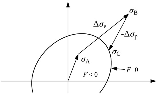
Figure 1.
Iteration diagram of the backward Euler algorithm.
According to the orthogonal flow rule of plasticity theory, the plastic strain rate can be expressed as
In the formula, G represents the plastic potential function, represents the plastic flow factor, and b is the first-order partial derivative of the potential function to the stress.
Therefore, in the constitutive integration algorithm, the first derivative of the yield function and the plastic potential function to the stress are required. Therefore, it is necessary to derive the two separately.
2.2. Anisotropic Plasticity Theory
ABAQUS uses the plastic potential function expression proposed by Menetrey and Willam [47]. It is hyperbolic on the meridian plane and elliptical on the π plane. As shown in Figure 2, the plastic potential surface is completely smooth, avoiding the singularity of the numerical integration at the corner of the Mohr–Coulomb yield function (Equation (2)). The Mohr–Coulomb correlation yield function is proposed in Appendix A to derive the vector a.
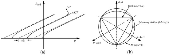
Figure 2.
Mohr–Coulomb plastic potential surface. (a) Plastic potential surface on the meridian plane; (b) The plastic potential surface on the deviatoric plane.
In Equation (2), ε represents the meridian eccentricity, which governs the resemblance between the hyperbolic shape of the plastic potential function on the meridian plane and its asymptote. The dilatancy angle, denoted by ψ, and the initial cohesion c|0 are also defined. The value of c|0 signifies the cohesion prior to any plastic deformation, and in the absence of hardening or softening, it remains constant. The triple symmetric elliptic form of the plastic potential function on the partial plane is denoted by Rmw(θ, e) and can be expressed using Equations (3) and (4).
In Equation (4), φ represents the friction angle of the soil, while e refers to the eccentricity on the π plane. The eccentricity e governs the shape of the plastic potential surface within the range of θ = 0 to π/3 on the π plane, as depicted in (Equation (5)).
Let the vector b denote the derivative of the plastic potential function G to the stress (Equation (6)).
where
Specifically expressed as
Since the expression of Rmw(θ, e) is more complex, for the convenience of derivation, a total of five temporary variables are recorded:
The following is available:
The partial derivatives of p, q, and θ to stress are consistent with the expressions in the yield function.
The expression of vector b is
It can be simplified as
2.3. UMAT Subroutine Call
The object of the UMAT subroutine during data transmission is the integral point of the unit. At the beginning of the incremental step, the main program will enter the UMAT through the UMAT interface and pass the initial value of the important variable to the unit integral point. At the end of the UMAT call, the updated variables will return to the main program through the interface, and the complete call process of the user material subroutine UMAT is shown in Figure 3.
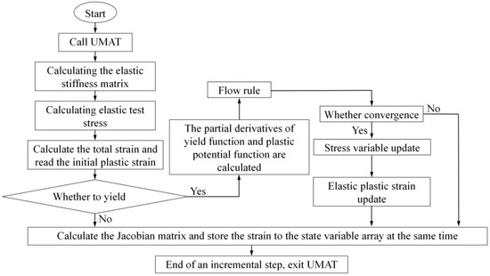
Figure 3.
UMAT call process.
3. Finite Element Analyses
3.1. General Description
Utilizing the finite element software ABAQUS, a three-dimensional model of a pile-supported embankment was constructed, encompassing the four main components: soft soil, pile structure, embankment fill, and geogrid. In order to ensure computational efficiency, a model containing 1/4 pile is established according to the symmetry of the model, as shown in Figure 4. The soft soil layer has a thickness of 10 m in the model, while the embankment has a height of 6.5 m. The pile cap is square-shaped with a side length of 0.5 m and a thickness of 0.5 m. The piles have a length of 9.5 m and a width of 0.5 m, and they are spaced at intervals of 2.5 m. A layer of geogrid with a stiffness of 3 MN/m is also considered, at a small height of 0.1 m above the base of the embankment. The overall size of the model is shown in Figure 4.
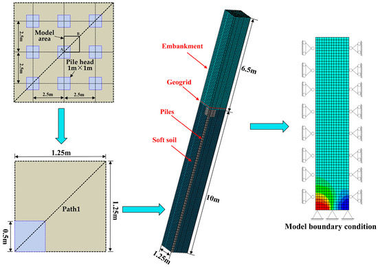
Figure 4.
Finite element model of pile-supported embankment.
For the displacement boundary conditions, the displacement at the bottom and around the model is not allowed. For the hydraulic boundary conditions, a diving level is set on the upper surface of the clay layer to generate a hydrostatic pore water pressure distribution in the area, which means that water is allowed to drain through the upper surface of the soft clay. In the FE models, the 8-node solid pore pressure element (C3D8P) is used for soft clay, and the 8-node solid element (C3D8) is used for piles and embankment fill. The geogrid is represented by a fully integrated first-order four-node quadrilateral membrane element (M3D4) [48].
3.2. Constitutive Models
In terms of this numerical model, the modified Cam-clay model is used for the soft clay layer, the improved Mohr–Coulomb model is used for embankment filling, and the elastic model is used for both piles and geogrids, in which the pile material is concrete. The material parameters of each model are derived from Zhuang and Ellis (2016) [48], as shown in Table 1 and Table 2. The interface friction angle between the geogrid and embankment adopts the hypothesis proposed by Liu and Goh [49], and the interface friction angle between the embankment fill and geogrid is approximately equal to the friction angle of the embankment fill. The interface friction angle between the pile and subsoil can be confirmed by Equation (18) [50]. In order to facilitate clear delineation and consistent expression, the center position of the pile cap is marked as point A, the center position of the four piles is marked as point B, and the path of the geogrid from point A to point B is defined as path 1, as shown in Figure 3.
where φ is the friction angle of the soil. In this analysis, it is assumed that the ratio of the interface friction angle φi to the soil friction angle φ is 0.7.

Table 1.
Material parameters of pile and fill.
Table 2.
Material parameters of soft soil.
3.3. Simulation Procedure
In the calculation and analysis, the simulation is divided into three stages. In the first stage, the ground stress balance of soft soil and pile is carried out. In the second stage, the in situ stress balance of the embankment is carried out. In this analysis step, the same supporting force as the self-weight of the embankment is set at the bottom of the embankment, so as to eliminate the settlement of the embankment under the self-weight. In the third stage, the support force is gradually reduced to zero, and the embankment deformation and stress distribution caused by soft soil compression under the action of embankment gravity are simulated.
3.4. Calibration Results
To evaluate the computational accuracy of the UMAT implementation, a comparative analysis was conducted with results obtained from the ABAQUS source programs. The analysis involved using a cohesion value of 5 kPa and a friction angle of 30°. Figure 5 depicts the embankment settlement curve determined by both the ABAQUS source program and UMAT. The settlement obtained from the ABAQUS source program measures 114.7 mm, while the UMAT implementation yields a settlement of 114.3 mm. This indicates a negligible maximum error of 1%. In addition, the calculation results of both the source program and UMAT at the top of the embankment are consistent, both of which are 83.7 mm. By comparing the calculation results of the ABAQUS source program and UMAT, it can be seen that the UMAT subroutine written in this paper is in good agreement with the calculation results of the source program, and the calculation accuracy is high. Therefore, it is feasible to develop an anisotropic yield criterion based on the current UMAT.
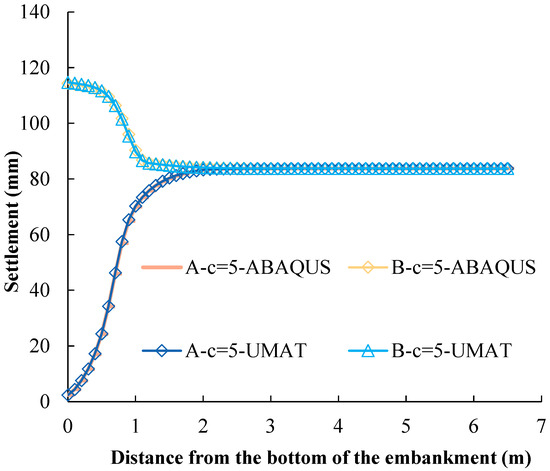
Figure 5.
The influence of the distance from the bottom of the embankment on the embankment settlement.
4. Soil Arching Considering the Cohesion Anisotropy
4.1. Cohesion Anisotropy
Chen and Snitbhan [51] (1974) conducted a study on the cohesion of soil slopes, considering the variability of soil characteristics based on the principal stress direction. They treated cohesion c as a variable that depends on the orientation of the principal stresses. To analyze the stability of soil slopes, they employed two types of cohesion parameters: vertical cohesion cv and horizontal cohesion ch. These parameters accounted for the increase in cohesion linearly and unevenly with depth. This approach offers a more comprehensive understanding of the factors influencing slope stability in geotechnical engineering. The anisotropic cohesion ci, can be expressed as:
where cv, ch, represent the cohesion in the vertical direction and horizontal direction, respectively; i represents the angle between the large principal stress and the vertical direction, which is determined by the following formula in the two-dimensional case:
where σx, σz, and τxz represent horizontal stress, vertical stress, and shear stress, respectively.
In the context of three-dimensional geotechnical analysis, the soil is considered to exhibit transverse isotropy [52]. The principal stress direction angles within the xz plane are ascertained by σx, σz, and τxz, while those in the yz plane are ascertained by σy, σz, and τyz. These calculations yield the corresponding directional angles for both planes. Consequently, the larger angle values from them were adopted to compute the cohesive forces at the location of the integration point.
If the anisotropy coefficient k is defined as , Equation (19) can be expressed as:
To consider the anisotropy of cohesion, the Mohr–Coulomb yield function replaces the constant c with ci, resulting in the Mohr–Coulomb yield criterion (Equation (23)).
4.2. Cohesion Parameter Analysis
To analyze the influence of the anisotropy degree of cohesion on the stress distribution and settlement of embankments, we selected a cohesion value of cv = 5 kPa and defined different anisotropy coefficients to quantify the degree of anisotropy. The friction angle was assumed to be isotropic at 30°. Based on the analysis results from Reference [53], we considered anisotropic coefficients of cohesion as 0.7, 0.5, and 0.3. The ci values under different anisotropic coefficients k of cohesive force were calculated using Equation (23). Figure 6 illustrates the variation of ci with the direction angle i of the major principal stress. When i = 0°, ci reaches its maximum value cv; when i = 90°, ci takes the minimum value ch. For values of i between 0° and 90°, ci shows a nonlinear decreasing trend. Please refer to Table 3 for the model plan of the study on anisotropic cohesion.
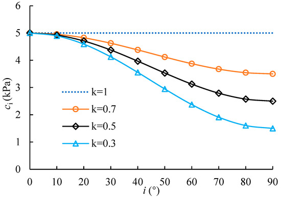
Figure 6.
Variation of the cohesive force in terms of i for various values of k.
Table 3.
Anisotropic cohesion research model plan.
4.3. The Stress Distribution in Embankments Is Influenced by the Anisotropy of Cohesive Force
In order to study the influence of cohesion anisotropy on the stress distribution in embankments, the distribution of major principal stress and the change of pile–soil stress ratio under different degrees of cohesion anisotropy are analyzed, respectively. Figure 7 shows the vector diagram of the major principal stress of the embankment with different anisotropy coefficients k. It can be seen from the figure that the direction of the major principal stress at the center of the two piles is close to the horizontal direction in the range of 0–1.5 m. At the same height in the embankment, from the center of the two piles to the upper position of the pile top, the major principal stress gradually deflects from the horizontal direction to the vertical direction and points to the pile top. As the anisotropy coefficient decreases, the major principal stress above the pile top decreases, indicating that the anisotropy leads to a decrease in strength, which weakens the horizontal transmission effect of vertical stress. This is consistent with Wang and Jin’s [53] proposal that ‘with the application of gravity load, the major principal stress gradually turns to the vertical direction’.
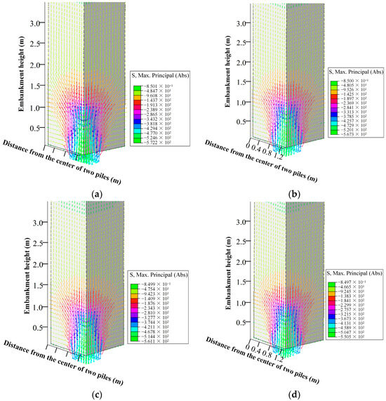
Figure 7.
Vector diagram of the major principal stress in embankment (kPa): (a) k = 1; (b) k = 0.7; (c) k = 0.5; (d) k = 0.3.
In the UMAT subroutine, the cohesive force is stored by the fourteenth state variable (SDV14). Figure 8 shows the anisotropic cohesive force distribution when the embankment model calculation is completed. It can be seen from the figure that the cohesion changes with the direction of the major principal stress. The closer to the center of the two piles, the smaller the cohesion, indicating that the vertical stress at this position is no longer the major principal stress, and the direction of the major principal stress tends to be horizontal.
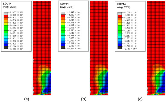
Figure 8.
Anisotropic distribution of the cohesion in embankment (kPa): (a) k = 0.77; (b) k = 0.5; (c) k = 0.3.
When the cohesive force cv = 5 kPa, the variation of the pile–soil stress ratio with the differential settlement in the embankment is shown in Figure 9. It can be seen from Figure 9 that with the increase in differential settlement, the pile–soil stress ratio gradually increases. When the differential settlement is less than 38 mm, the pile–soil stress ratio increases significantly. When the differential settlement is greater than 38 mm, the pile–soil stress ratio increases marginally. On the whole, with the increase in anisotropy, the pile–soil stress ratio decreases. It can be seen from the end point of the curve that the increase in anisotropy not only causes the increase in settlement but also leads to the decrease in the pile–soil stress ratio. This is consistent with Oliveira and Lemos [54] ‘anisotropic MIT-E3 elastoplastic constitutive model can produce greater vertical displacement’. The pile–soil stress corresponding to different anisotropy coefficients is shown in Figure 10. It can be seen that the pile–soil stress ratio is inversely proportional to the degree of anisotropy. The soil arching effect in the embankment depends on the shear stress in the soil. At this time, the major principal stress of the soil element in the soil arching range is no longer in the vertical direction. The stronger the anisotropy is, the more the cohesion decreases. Therefore, as the anisotropy coefficient decreases, the pile–soil stress ratio decreases gradually. As the anisotropy coefficient decreases from 1 to 0.3, the pile–soil stress ratio decreases from 36.1 to 28.8.
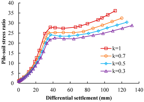
Figure 9.
Influence of the pile–soil stress ratio on differential settlement of the embankment.
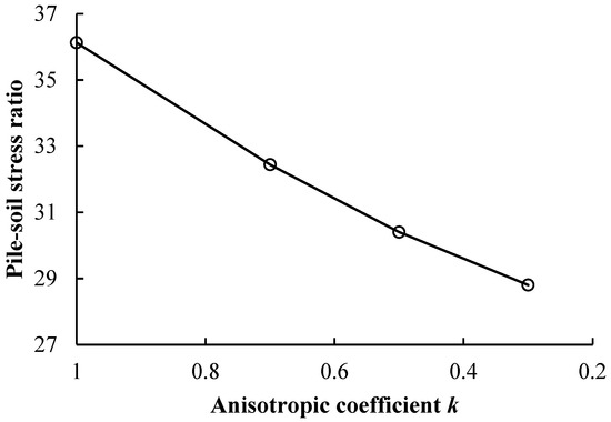
Figure 10.
Influence of the cohesion anisotropy coefficient on the pile–soil stress ratio.
4.4. The Tensile Stiffness of Geogrid Is Affected by the Anisotropy of Cohesion
Geogrid is an important part of effectively distributing the internal stress of embankment structures in geotechnical engineering. In order to study the influence of cohesion anisotropy on the mechanical properties of geogrid, it is necessary to analyze its tensile stress behavior. Figure 11 shows the tensile stress curve of geogrid along path 1. It can be seen from the diagram that the main growth of tensile stress along path 1 occurs in the area corresponding to the pile cap, and the peak stress appears at the edge of the pile cap. This has a good correspondence with the research results of Jones [55] and Halvordson [56]. It is mainly due to the formation of a rigid support point at the connection between the geogrid and the pile at the edge of the pile cap. Near this support point, the load will be transmitted to the pile body through the geogrid, leading to an increase in stress. As the anisotropy coefficient k decreases from 1 to 0.3, the maximum tensile stress along path 1 increases significantly by 15.5%, from 56.1 MPa to 64.8 MPa. Therefore, in the design and application of geogrids, it is necessary to fully consider the anisotropy of soil cohesion. The mechanical properties of the soil are fully investigated and tested to ensure that the mechanical properties of the geogrid meet the engineering requirements.
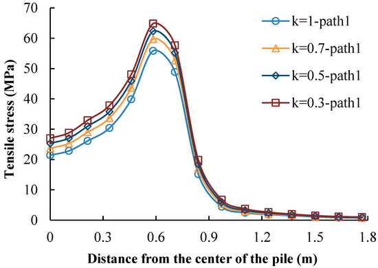
Figure 11.
The influence of the distance from the center of four piles on the tensile stress of geogrids.
4.5. Embankment Settlement Is Affected by the Anisotropy of Cohesion
Figure 12 shows the influence of different degrees of anisotropy of cohesion on the vertical settlement of the embankment. A represents the position of the pile top, and B represents the center position of four piles. It can be seen that the stronger the anisotropy of cohesion, the larger the settlement of the embankment. The minimum settlement of the embankment is the contact position between the bottom of the embankment and the pile cap, and the maximum settlement is the center position of the four piles at the bottom of the embankment. It can be seen from the figure that the settlement value is consistent within a certain height to the top surface of the embankment. From the same level to the top of the pile, the settlement gradually decreases. From the same level to the center of the four piles at the bottom of the embankment, the settlement gradually increases. When the anisotropy coefficient is different, the position of the equal settlement surface is about 2.3 m, so the change of cohesion caused by the anisotropy coefficient has little effect on the position of the equal settlement surface. The variation in settlement with changes in the anisotropy coefficient is shown in Figure 13. Combined with Figure 12, it can be seen that when the anisotropy coefficient decreases from 1 to 0.3, the maximum settlement increases from 114.7 mm to 134.2 mm, an increase of 17.0%. The settlement of the top surface of the embankment increases from 83.7 mm to 93.8 mm, an increase of 12.1%, indicating that the anisotropy of the cohesive force has a significant impact on the settlement of the embankment.
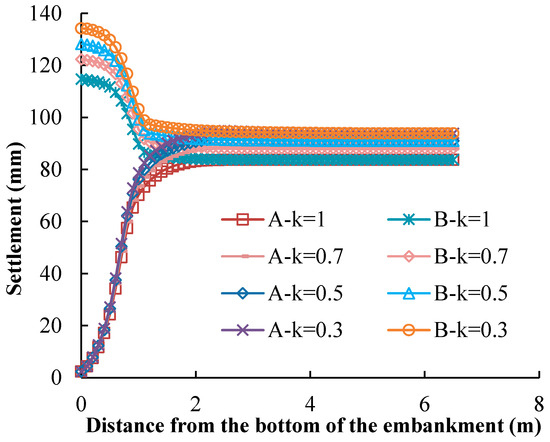
Figure 12.
Effect of the anisotropy coefficient k on embankment settlement.
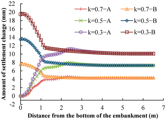
Figure 13.
Influence of the anisotropic coefficient k on the settlement variation of the embankment.
5. Soil Arching Considering Friction Angle Anisotropy
Under the action of self-weight, the long axis of the soil particles tends to be parallel to the sedimentary surface. Therefore, under the action of horizontal shear stress, the sliding surface is easier to form, and the shear strength is lower. Under the action of vertical shear stress, the soil particles are prone to dislocation and rearrangement, the sliding surface is more difficult to produce, and the shear strength is higher. The experimental research of relevant scholars [57] shows that the friction angle of soil is closely related to the direction of principal stress, and the strength of soil in different loading directions is obviously different. Therefore, an accurate understanding of friction angle anisotropy is helpful to accurately evaluate the shear strength and bearing capacity of soil and predict the risk of landslides and instability in embankment engineering.
In order to analyze the influence of the anisotropy of the internal friction angle on the stress distribution and deformation development of the embankment, this chapter will use the Mohr–Coulomb material subroutine UMAT in the analysis of the three-dimensional pile-supported embankment model and embed the Section 5.1 of the anisotropic internal friction angle calculation formula in the yield function of the subroutine to realize the dynamic change of the anisotropy of the internal friction angle in the numerical calculation and analysis.
5.1. Friction Angle Anisotropy
Based on the Mohr–Coulomb yield criterion, in the finite element calculation, the value of the friction angle at each integral point is regarded as a function of the shear stress direction, and it is developed into a yield criterion that can consider the anisotropy of the friction angle. For the calculation of the friction angle, the calculation formula proposed by Schweiger [58,59] is derived from the fabric tensor A proposed by Pietruszczak and Mroz [60] from the microscopic point of view. For orthotropic materials, A can be expressed by Equation (24):
where a1, a2 and a3 are eigenvalues of tensors. By introducing the unit vector n, the scalar value α of tensor A in different directions in the orthogonal coordinate systems e(1), e(2), and e(3) can be obtained. As shown in Formula (25), any material parameter value in the n direction can be considered according to Formula (25).
The normalized partial tensor of vector A is
For isotropic materials:
where . By combining Formulas (25) and (26), and assuming that the anisotropy coefficient of the difference between vertical and horizontal strength is Ar (anisotropy ratio), the calculation formula for strength parameters in the n direction can be obtained, as shown in Formula (28):
where , nv denotes the vertical component of the unit vector n. Therefore, the anisotropic internal friction angle can be calculated using Equation (29):
where , , φ0 represents the average value of the friction angle in each direction; φv and φh are the friction angles when the shear stress direction is vertical and horizontal, respectively.
In the calculation of the model, the strength of the soil is the largest when the vertical shear is considered, and the strength is the smallest when the horizontal shear is considered. Therefore, the nv value is determined by the angle between the shear stress and the vertical direction at different stress states, and φ′ is brought into the Mohr–Coulomb yield function. The Mohr–Coulomb yield criterion considering the anisotropy of the internal friction angle can be obtained:
When calculating and analyzing, it is necessary to input the internal friction angle anisotropy coefficient (Ar) value in the user-defined material parameter window. For specific projects, it should be accurately obtained through multiple sets of tests.
5.2. Friction Angle Parameter Analysis
In order to study the influence of the anisotropy degree of friction angle on the stress distribution and settlement in embankment, the anisotropy degree of friction angle is defined by setting different anisotropy coefficients for the condition that the friction angle φ of cohesionless soil measured by triaxial test is 30°. According to the measured values of φv and φh in Reference [52], it can be seen that the anisotropy coefficient (Ar) of the friction angle is less than 1.5. Therefore, this paper only studies the influence of the anisotropy of friction angle on embankment structure in this range. Figure 14 is the variation curve of the friction angle with the direction of shear stress θ when the anisotropy coefficients of different friction angles are calculated according to Equation (29). When the shear stress direction is vertical, the shear strength of the soil is fully exerted, and the friction angle takes the maximum value φv; when the shear stress direction is horizontal, the shear strength of the soil is the smallest, and the friction angle takes the minimum value φh. When the value of θ is 45-φv/2, the friction angle is 30°. The friction angle anisotropy research model plan is shown in Table 4. In the finite element analysis, the cohesion cannot be set to zero, so it is taken as 0.1 kPa.
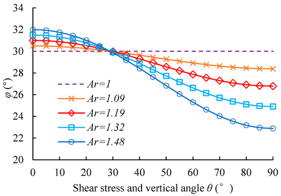
Figure 14.
Variation of the friction angle in terms of for various values of (Ar).
Table 4.
Anisotropy of the friction angle research model plan.
In the UMAT program, the friction angle is stored by the fifteenth state variable (SDV15). Figure 15 shows the distribution of the friction angle anisotropy coefficient when the model calculation is completed. Consistent with the anisotropic distribution of cohesion, the pile top position and the area outside the influence range of soil arching are not affected. The friction angle near the center of the two piles decreases, but the minimum value is not at the center of the two piles, indicating that the shear stress at the center of the two piles is not horizontal.
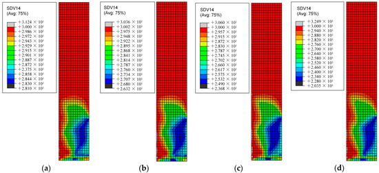
Figure 15.
Anisotropic friction angle distribution (°): (a) Ar = 1.09; (b) Ar = 1.19; (c) Ar = 1.32; (d) Ar = 1.48.
5.3. The Stress Distribution of Embankment Is Affected by the Anisotropy of Friction Angle
In order to understand the influence of anisotropic friction angle on the internal stress distribution of embankments, the change of the pile–soil stress ratio under different anisotropy degrees of friction angle is comprehensively analyzed. Figure 16 is the variation curve of the pile–soil stress ratio with differential settlement. It can be seen from Figure 16 that as the friction angle anisotropy coefficient increases, the pile–soil stress ratio gradually decreases and the differential settlement gradually increases. It shows that the part of the load transferred to the top of the pile through the shear stress is reduced. Therefore, the anisotropy of the friction angle significantly affects the degree of the soil arching effect. When the anisotropy is enhanced, the soil arching effect is weakened.
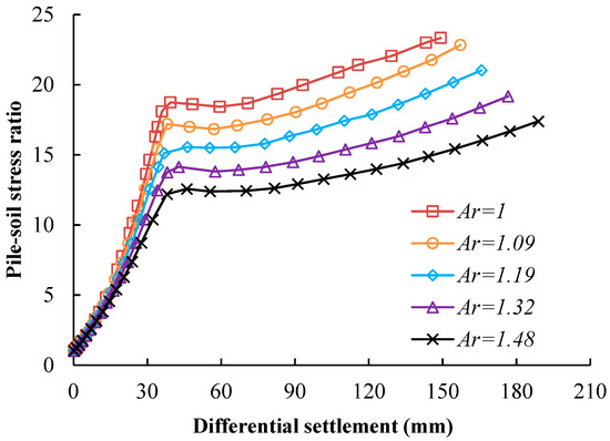
Figure 16.
Effect of the friction angle anisotropy coefficient (Ar) on the pile–soil stress ratio.
5.4. The Tensile Stiffness of Geogrid Is Affected by the Anisotropy of Friction Angle
Figure 17 illustrates the tensile stress curve along path 1 for the geogrid. The geogrid experiences a gradual increase in tensile stress as the anisotropy coefficient rises. Notably, the upward trend in tensile stress along path 1 is primarily concentrated within the range of the pile cap, with the highest value observed at the corner of the pile cap. With an increase in the anisotropy coefficient (Ar) from 1 to 1.48, the maximum tensile stress along path 1 rises by 27.8%, from 72.9 MPa to 93.2 MPa.
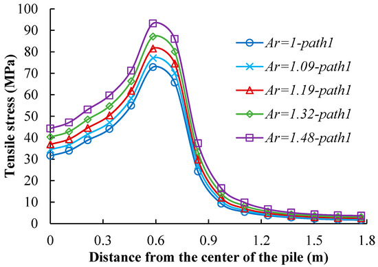
Figure 17.
Effect of the friction angle anisotropy coefficient (Ar) on the stress distribution of geogrid.
5.5. Embankment Settlement Is Affected by Friction Angle Anisotropy
In investigating the impact of the anisotropy degree pertaining to the friction angle on embankment settlement, it is imperative to analyze the computational outcomes concerning the vertical displacement of embankments exhibiting distinct anisotropy coefficients allied with their respective friction angles (Ar). Figure 18 illustrates the vertical settlement curve of the embankment with varying anisotropy coefficients of the friction angle (Ar), in accordance with the aforementioned discussion. Position A represents the location above the pile top, while position B represents the central position of the four piles. It is evident that the embankment settlement increases significantly with an increasing anisotropy coefficient. The settlement curve tends to stabilize at the position of the iso-settling surface. The position of the iso-settling surface undergoes minimal change, approximately 2.3 m, with an increasing anisotropy coefficient of the friction angle.
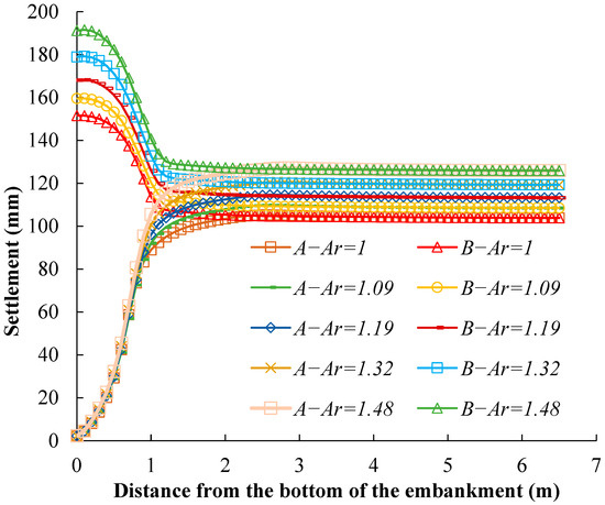
Figure 18.
The influence of different (Ar) values on embankment settlement.
As depicted in Figure 19, an increase in the anisotropy coefficient from 1 to 1.48 leads to a corresponding increase in the maximum embankment settlement from 151.6 mm to 191.2 mm, representing a 26.1% increase. Additionally, the settlement at the top of the embankment increases by 21.2% from 103.9 mm to 125.9 mm. These observations highlight the substantial influence of the anisotropy of the friction angle on the settlement of the embankment.
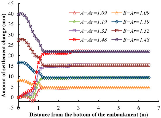
Figure 19.
The influence of different (Ar) values on the settlement variation of the embankment.
6. Engineering Example Verification and Related Design Description
6.1. Engineering Example Verification
In order to further verify the accuracy of the anisotropic yield criterion in this paper, the existing engineering examples [61] are selected. The finite element model consistent with the example is established by ABAQUS, and the analysis steps corresponding to the field are set up. The anisotropic Mohr–Coulomb yield criterion is applied to the embankment, and the numerical results under isotropic and anisotropic conditions are compared with the measured results to analyze the influence of anisotropy on the mechanical properties of the embankment structure. The results show that the settlement of embankment increases gradually with the increase in anisotropy coefficient of embankment. The maximum settlement of the embankment under isotropic conditions is 93.4 mm. When the anisotropy coefficient (Ar) is 1.1 and 1.2, the settlement increases to 95.7 mm and 103.3 mm, respectively, with an increase of 2.5% and 10.6%. The measured and simulated values of the maximum settlement in the center of the embankment in Reference [61] are 104 mm and 92.5 mm, respectively. Therefore, when the anisotropy coefficient (Ar) = 1.2, the model calculation results are in good agreement with the field-measured values. It shows that the embankment fill has a certain degree of anisotropy and also further verifies the rationality and applicability of the numerical calculation method in this paper.
6.2. Anisotropic Soil Construction Design
It is assumed that in the vertical direction of the embankment (along the elevation direction), the shear strength of the soil is larger, while in the transverse direction of the embankment (along the width direction of the embankment), the shear strength of the soil is smaller. In this case, for the embankment design, the following measures can be taken:
- (1)
- Filler direction: determine the layout direction of the filler layer to make full use of the high shear strength of the soil in the direction perpendicular to the embankment. The preferred direction of the filler can be selected to be consistent with the longitudinal direction of the vertical embankment to improve the overall stability of the embankment.
- (2)
- Filler type and thickness: Considering the low shear strength of the soil in the transverse direction of the embankment, high-strength filler material can be selected or the thickness of the filler layer can be increased to improve the bearing capacity of the embankment in the transverse direction.
- (3)
- Foundation treatment: According to the research results of soil anisotropy, appropriate foundation treatment measures can be considered, such as reducing pile spacing or increasing multi-layer geogrid, so as to further improve the stability of the embankment in different directions.
7. Conclusions
In this study, the significance of anisotropic behavior in embankment fill materials was addressed. An anisotropic calculation formula incorporating strength parameters was proposed, and a modified Mohr–Coulomb criterion was introduced. To investigate the influence of anisotropy on the stress and settlement of embankments, a customized user-defined subroutine (UMAT) was developed. The key findings and research contributions of this study were summarized as follows:
- (1)
- The Mohr–Coulomb yield criterion incorporates anisotropic considerations for cohesion, treating cohesion as a function of the direction of the principal stress. This approach enables dynamic updates of cohesion with changes in the direction of major principal stress in the code. When examining the effects of anisotropy on pile–soil stress ratios with a cohesive strength of 5 kPa, it was observed that as the anisotropy of cohesion intensifies and the anisotropy coefficient diminishes from 1 to 0.3, the ratio decreases from 36.1 to 28.8. Additionally, there is a notable 12.1% increase in settlement at the top of the embankment, highlighting the impact of cohesion anisotropy on geotechnical structural performance.
- (2)
- This paper presents an advancement of the Mohr–Coulomb criterion by incorporating a variable function that represents the dependence of friction angles on the direction of shear stress. This extension allows for the consideration of friction angle anisotropy in the material subroutine, enhancing the accuracy and adaptability of the yield criterion. Through an investigation of cases with a fixed friction angle of 30°, it was observed that as the coefficient of friction angle anisotropy increased from 1 to 1.48, resulting in heightened anisotropy, the pile–soil stress ratio experienced a significant decrease, dropping from 23.7 to 17.4. Additionally, the friction angle anisotropy exhibited a correspondence with an increased settlement at the pinnacle of the embankment, with the settlement of the top surface of the embankment increasing by 21.2%.
- (3)
- A numerical model consistent with the existing model test and field test is established. By comparing the field test results with the numerical calculation results using the anisotropic Mohr–Coulomb yield criterion, it is found that the calculation results under anisotropic conditions are closer to the actual situation than isotropic, which verifies the accuracy and applicability of the anisotropic numerical calculation method in this paper.
Author Contributions
Conceptualization, Y.Z.; writing—original draft preparation, Y.Z. and H.F.; writing—review and editing, Y.W. and J.L.; visualization, Y.Z. and J.C.; funding acquisition, Y.Z. and Z.C. All authors have read and agreed to the published version of the manuscript.
Funding
This research was funded by the National Natural Science Foundation for the General Program of China (Grant No. 52178316) and the National Science Fund for Excellent Young Scholars of China (Grant No. 51922029).
Institutional Review Board Statement
Not applicable.
Informed Consent Statement
Not applicable.
Data Availability Statement
All data that support the findings of this study are included within the article.
Conflicts of Interest
The authors declare no conflict of interest.
Nomenclature
| Serial number | Parameter | Definition |
| 1 | plastic flow factor | |
| 2 | G | plastic potential function |
| 3 | plastic strain rate | |
| 4 | σ | stress |
| 5 | b | derivative of the plastic potential function G to the stress |
| 6 | Rmc | yield curve shape of the yield function on the partial plane |
| 7 | p | average stress |
| 8 | ε | meridian eccentricity |
| 9 | c|0 | initial cohesion |
| 10 | ψ | dilatancy angle |
| 11 | Rmw(θ, e) | triple symmetric elliptic form of the plastic potential function on the partial plane |
| 12 | q | deviatoric stress |
| 13 | θ | Lode angle |
| 14 | e | eccentricity on the π plane |
| 15 | φ | friction angle of the soil |
| 16 | I | identity matrix |
| 17 | φi | interface friction angle |
| 18 | E | elastic modulus |
| 19 | v | Poisson ratio |
| 20 | c | cohesion |
| 21 | γ | unit weight |
| 22 | λ | compression index |
| 23 | κ | rebound index |
| 24 | M | critical state stress ratio |
| 25 | γʹ | soft soil unit weight |
| 26 | e1 | intercept of the slope of the e-lnp normal consolidation curve |
| 27 | ci | anisotropic cohesion |
| 28 | ch | horizontal cohesion |
| 29 | cv | vertical cohesion |
| 30 | i | angle between the large principal stress and the vertical direction |
| 31 | σx | horizontal stress |
| 32 | σz | vertical stress |
| 33 | τxz | shear stress |
| 34 | k | anisotropy coefficient |
| 35 | n | unit vector |
| 36 | nv | vertical component of the unit vector n. |
| 37 | φ0 | friction angle in each direction |
| 38 | φv | vertical friction angle in the direction of shear stress |
| 39 | φh | horizontal friction angle in the direction of shear stress. |
| 40 | Ar | anisotropy ratio |
| 41 | r | third deviatoric stress invariant |
| 42 | S | deviatoric stress |
| 43 | a | first derivative of the yield function with respect to stress |
Appendix A
The yield function expression of the Mohr–Coulomb yield criterion in ABAQUS is expressed by the stress invariant (Equation (A1)) [62].
where
Rmc defines the yield curve shape of the yield function on the partial plane;
is the average stress;
defines the angle of polarization, namely, the Lode angle. When defined by the cosine function, the Lode angle ranges from 0 to 60°;
defines the third deviatoric stress invariant;
defines the deviatoric stress;
S defines the deviatoric stress, S = ;
I defines the identity matrix.
The yield function and plastic potential function are derived using the implicit integration algorithm. We denote the first derivative of the yield function with respect to stress as vector a (Equation (A3)).
where
Specifically expressed as
The derivative of the average principal stress p to stress is
The derivative of the generalized shear stress q with respect to stress is as follows:
The derivative of Lode angle θ to stress is expressed as
where the derivative of the third stress invariant to the stress multiplied by 27/2 is the derivative of r3 to the stress (Equation (A10)).
The derivatives of Lode angle θ with respect to mean principal stress p and generalized shear stress q are
The expression of vector a is
References
- Krabbenhøft, K.; Krabbenhøft, J. Simplified kinematic hardening plasticity framework for constitutive modelling of soils. Comput. Geotech. 2021, 138, 104146. [Google Scholar] [CrossRef]
- Arthur, J.R.F.; Menzies, B.K. Inherent Anisotropy in a Sand. Géotechnique 1973, 22, 115–128. [Google Scholar] [CrossRef]
- Lade, P.; Abelev, A. Characterization of Cross-Anisotropic Soil Deposits from Isotropic Compression Tests. Soils Found. 2005, 45, 89–102. [Google Scholar] [CrossRef] [PubMed]
- Abelev, A.V.; Lade, P.V. Characterization of Failure in Cross-Anisotropic Soils. J. Eng. Mech. 2004, 130, 599–606. [Google Scholar] [CrossRef]
- Azami, A.; Pietruszczak, S.; Guo, P. Bearing Capacity of Shallow Foundations in Transversely Isotropic Granular Media. Int. J. Numer. Anal. Methods Geomech. 2010, 34, 771–793. [Google Scholar] [CrossRef]
- Symes, M.J.; Genst, A.; Hight, D.W. Drained Principal Stress Rotation in Saturated Sand. Géotechnique 1988, 38, 59–81. [Google Scholar] [CrossRef]
- Symes, M.J.P.R.; Gens, A.; Hight, D.W. Undrained Anisotropy and Principal Stress Rotation in Saturated Sand. Géotechnique 1984, 34, 11–27. [Google Scholar] [CrossRef]
- Zamanian, M.; Mollaei-Alamouti, V.; Payan, M. Directional Strength and Stiffness Characteristics of Inherently Anisotropic Sand: The Influence of Deposition Inclination. Soil Dyn. Earthq. Eng. 2020, 137, 106304. [Google Scholar] [CrossRef]
- Daraei, A.; Herki, M.B.; Sherwani, H.F.A.; Shokrollah, Z. Rehabilitation of Portal Subsidence of Heybat Sultan Twin Tunnels: Selection of Shotcrete or Geogrid Alternatives. Int. J. Geosynth. Ground Eng. 2018, 4, 15. [Google Scholar] [CrossRef]
- Daraei, A.; Herki, A.M.B.; Sherwani, H.F.A.; Zare, S. Slope Stability in Swelling Soils Using Cement Grout: A Case Study. Int. J. Geosynth. Ground Eng. 2018, 4, 10. [Google Scholar] [CrossRef]
- Arthur, J.R.F.; Chua, K.S.; Dunstan, T. Induced Anisotropy in a Sand. Géotechnique 1977, 27, 13–30. [Google Scholar] [CrossRef]
- Mahmoudi, M.; Rajabi, A.M. A numerical simulation using FLAC3D to analyze the impact of concealed karstic caves on the behavior of adjacent tunnels. Nat. Hazards 2023, 117, 555–577. [Google Scholar] [CrossRef]
- Meiqin, L.; Shang, W.; Fei, P. Simulation and Analysis of Three-point Bending Experiment with Hollow Beam Based on Abaqus. J. Phys. Conf. Ser. 2023, 2566, 012063. [Google Scholar] [CrossRef]
- Wang, L.F.; He, X.Q.; Sun, Y.Z.; Liew, K.M. A mesh-free vibration analysis of strain gradient nano-beams. Eng. Anal. Bound. Elem. 2017, 84, 231–236. [Google Scholar] [CrossRef]
- Ma, X.; Kiani, K. Spatially nonlocal instability modeling of torsionaly loaded nanobeams. Eng. Anal. Bound. Elem. 2023, 154, 29–46. [Google Scholar] [CrossRef]
- Kiani, K. Nanomechanical sensors based on elastically supported double-walled carbon nanotubes. Appl. Math. Comput. 2015, 270, 216–241. [Google Scholar] [CrossRef]
- Peng, L.X.; Liew, K.M.; Kitipornchai, S. Buckling and free vibration analyses of stiffened plates using the FSDT mesh-free method. J. Sound Vib. 2006, 289, 421–449. [Google Scholar] [CrossRef]
- Kiani, K. Column buckling of magnetically affected stocky nanowires carrying electric current. J. Phys. Chem. Solids 2015, 83, 140–151. [Google Scholar] [CrossRef]
- Zhang, L.W.; Zhang, Y.; Liew, K.M. Modeling of nonlinear vibration of graphene sheets using a meshfree method based on nonlocal elasticity theory. Appl. Math. Model. 2017, 49, 691–704. [Google Scholar] [CrossRef]
- Kiani, K. Nonlocal discrete and continuous modeling of free vibration of stocky ensembles of vertically aligned single-walled carbon nanotubes. Curr. Appl. Phys. 2014, 14, 1116–1139. [Google Scholar] [CrossRef]
- Bu, N.; Zhang, Y.; Li, X.; Chen, W.; Jiang, C. Contact High-Temperature Strain Automatic Calibration and Precision Compensation Research. J. Artif. Intell. Technol. 2022, 2, 69–76. [Google Scholar] [CrossRef]
- Du, H.; Du, S.; Li, W. Probabilistic time series forecasting with deep non-linear state space models. CAAI Trans. Intell. Technol. 2023, 8, 3–13. [Google Scholar] [CrossRef]
- Benali, A.; Hachama, M.; Bounif, A.; Nechnech, A.; Karray, M. A TLBO-optimized artificial neural network for modeling axial capacity of pile foundations. Eng. Comput. 2021, 37, 675–684. [Google Scholar] [CrossRef]
- Chen, J.; Yu, S.; Wei, W.; Ma, Y. Matrix-based method for solving decision domains of neighbourhood multigranulation decision-theoretic rough sets. CAAI Trans. Intell. Technol. 2022, 7, 313–327. [Google Scholar] [CrossRef]
- Yao, Z.W.; Huang, Q.; Ji, Z.; XF, L.; Bi, Q. Deep learning-based prediction of piled-up status and payload distribution of bulk material. Autom. Constr. 2021, 121, 103424. [Google Scholar] [CrossRef]
- Che, J.; Tong, X.; Yu, L. A dynamic bidirectional heuristic trust path search algorithm. CAAI Trans. Intell. Technol. 2022, 7, 340–353. [Google Scholar] [CrossRef]
- Wang, H.; Yue, W.; Wen, S.; Xu, X.; Haasis, H.D.; Su, M.; Liu, P.; Zhang, S.; Du, P. An improved bearing fault detection strategy based on artificial bee colony algorithm. CAAI Trans. Intell. Technol. 2022, 7, 570–581. [Google Scholar] [CrossRef]
- Jackson-Mills, G.; Barber, A.R.; Blight, A.; Pickering, A.; Boyle, J.H.; Richardson, R.C. Non-assembly 3D-printed walking mechanism utilising a hexapod gait. J. Artif. Intell. Technol. 2022, 2, 158–163. [Google Scholar] [CrossRef]
- Hsiao, I.H.; Chung, C.Y. AI-infused semantic model to enrich and expand programming question generation. J. Artif. Intell. Technol. 2022, 2, 47–54. [Google Scholar] [CrossRef]
- Li, Y.Q.; Goh, A.T.C.; Zhang, R.H.; Zhang, W.G. Stability charts for undrained clay slopes considering soil anisotropic characteristics. Bull. Eng. Geol. Environ. 2023, 82, 52. [Google Scholar] [CrossRef]
- Tian, Y.; Yao, Y.P. Constitutive modeling of principal stress rotation by considering inherent and induced anisotropy of soils. Acta Geotech. 2018, 13, 1299–1311. [Google Scholar] [CrossRef]
- Tian, Y.; Yao, Y. A simple method to describe three-dimensional anisotropic failure of soils. Comput. Geotech. 2017, 92, 210–219. [Google Scholar] [CrossRef]
- Yao, Y.; Tian, Y.; Gao, Z. Anisotropic UH model for soils based on a simple transformed stress method. Int. J. Numer. Anal. Methods Geomech. 2017, 41, 54–78. [Google Scholar] [CrossRef]
- Chen, L. Studay on the Anisotropy of Clay. Appl. Mech. Mater. 2012, 1931, 193–194. [Google Scholar] [CrossRef]
- Lade, P.V.; Rodriguez, N.M.; Van, D.E.J. Effects of Principal Stress Directions on 3D Failure Conditions in Cross Anisotropic Sand. J. Geotech. Geoenvironmental Eng. 2014, 140, 1–12. [Google Scholar] [CrossRef]
- Kirkgard, M.M.; Lade, P.V. Anisotropic Three-Dimensional Behavior of a Normally Consolidated Clay. Can. Geotechnical. J. 1993, 30, 848–858. [Google Scholar] [CrossRef]
- Lam, W.; Tatsuoka, F. Effects of Initial Anisotropic Fabric and σ2 on Strength and Deformation Characteristics of Sand. Soils Found. 1988, 28, 89–106. [Google Scholar] [CrossRef]
- Zdravkovic, L.; Potts, D.M.; Hight, D.W. The Effect of Strength Anisotropy on the Behaviour of Embankments on Soft Ground. Géotechnique 2002, 52, 447–457. [Google Scholar] [CrossRef]
- Bhasi, A.; Rajagopal, K. Numerical study of basal reinforced embankments supported on floating/end bearing piles considering pile–soil interaction. Geotext. Geomembr. 2015, 43, 524–536. [Google Scholar] [CrossRef]
- Van, S.J.M.; Bezuijen, A.; Lodder, H.J.; Van Tol, A.F. Model experiments on piled embankments. Part, I. Geotext. Geomembr. 2012, 32, 69–81. [Google Scholar] [CrossRef]
- Lai, H.; Zheng, J.; Zhang, J.; Zhang, R.; Cui, L. DEM analysis of “soil”-arching within geogrid-reinforced and unreinforced pile-supported embankments. Comput. Geotech. 2014, 61, 13–23. [Google Scholar] [CrossRef]
- Lade, P.V. Failure Criterion for Cross-Anisotropic Soils. J. Geotech. Geoenvironmental Eng. 2008, 134, 117–124. [Google Scholar] [CrossRef]
- Li, X.; Dafalias, Y.F. Constitutive Modeling of Inherently Anisotropic Sand Behavior. J. Geotech. Geoenvironmental Eng. 2002, 128, 868–880. [Google Scholar] [CrossRef]
- Li, X.; Dafalias, Y.F. Constitutive Framework for Anisotropic Sand Including Non-Proportional Loading. Géotechnique 2004, 54, 41–55. [Google Scholar] [CrossRef]
- Dafalias, Y.F.; Papadimitriou, A.G.; Li, X.S. Sand Plasticity Model Accounting for Inherent Fabric Anisotropy. J. Eng. Mech. 2004, 130, 1319–1333. [Google Scholar] [CrossRef]
- Jia, S.P.; Chen, W.Z.; Yang, J.P.; Chen, P.S. An elastoplastic constitutive model based on modified Mohr-Coulomb criterion and its numerical implementation. Rock Soil Mechanics. 2010, 31, 2051–2058. [Google Scholar] [CrossRef]
- Menetrey, P.H.; Willam, K.J. Triaxial Failure Criterion for Concrete and its Generalization. ACJ Struct. J. 1995, 92, 311–318. [Google Scholar] [CrossRef]
- Zhuang, Y.; Ellis, E.A. Finite-Element Analysis of a Piled Embankment with Reinforcement and Subsoil. Géotechnique 2016, 66, 596–601. [Google Scholar] [CrossRef]
- Liu, H.L.; Ng, C.W.W.; Fei, K. Performance of a geogrid-reinforced and pile-supported highway embankment over soft clay: Case study. J. Geotech. Geoenvironmental Eng. 2007, 133, 1483–1493. [Google Scholar] [CrossRef]
- Potyondy, J.G. Skin friction between various soils and construction materials. Geotechnique 1961, 11, 339–353. [Google Scholar] [CrossRef]
- Chen, W.F.; Snitbhan, N.; Fang, H.Y. Stability of Slopes in Anisotropic, Nonhomogeneous Soils. Can. Geotech. J. 1975, 12, 146–152. [Google Scholar] [CrossRef]
- Penava, D.; Ani, F.; Trajber, D.; Vig, M.; Sigmund, V. Three-dimensional micromodel of clay block masonry wall. Int. J. Mason. Res. Innov. 2016, 1, 282–305. [Google Scholar] [CrossRef]
- Wang, D.; Jin, X. Slope stability analysis by finite elements considering strength anisotropy. Rock Soil Mech. 2008, 29, 667–672. [Google Scholar] [CrossRef]
- Oliveira, V.J.P.; Lemos, J.L. Numerical predictions of the behaviour of soft clay with two anisotropic elastoplastic models. Comput. Geotech. 2011, 38, 598–611. [Google Scholar] [CrossRef][Green Version]
- Jones, B.M.; Plaut, R.H.; Filz, G.M. Analysis of geosynthetic reinforcement in pile-supported embankments. Part I: 3D plate model. Geosynth. Int. 2010, 17, 59–67. [Google Scholar] [CrossRef]
- Halvordson, K.A.; Plaut, R.H.; Filz, G.M. 2010. Analysis of geosynthetic reinforcement in pile-supported embankments. Part II: 3D cable-net model. Geosynth. Int. 2010, 17, 68–76. [Google Scholar] [CrossRef]
- Xv, P.; Shao, S.J.; Zhang, S. Strength criterion of cross-anisotropic Q3 loess. Chin. J. Geotech. Eng. 2018, 40, 116–121. [Google Scholar] [CrossRef]
- Schweiger, H.F.; Wiltafsky, C.; Scharinger, F. A Multilaminate Framework for Modelling Induced and Inherent Anisotropy of Soils. Géotechnique 2009, 59, 87–101. [Google Scholar] [CrossRef]
- Galavi, V.; Schweiger, H.F. A Multilaminate Model with Destructuration Considering Anisotropic Strength and Anisotropic Bonding. Soils Found. 2009, 49, 341–353. [Google Scholar] [CrossRef]
- Pietruszczak, S.; Mroz, Z. Formulation of Anisotropic Failure Criteria Incorporating a Microstructure Tensor. Comput. Geotech. 2000, 26, 105–112. [Google Scholar] [CrossRef]
- Fei, K.; Liu, H.L. Field test study and numerical analysis of a geogridreinforced and pile-supported embankment. Rock Soil Mech. 2009, 30, 1004–1012. [Google Scholar] [CrossRef]
- Sun, R.; Yang, J.S. Axisymmetric adaptive lower bound limit analysis for Mohr-Coulomb materials using Semidefinite programming. Comput. Geotech. 2021, 130, 103906. [Google Scholar] [CrossRef]


Disclaimer/Publisher’s Note: The statements, opinions and data contained in all publications are solely those of the individual author(s) and contributor(s) and not of MDPI and/or the editor(s). MDPI and/or the editor(s) disclaim responsibility for any injury to people or property resulting from any ideas, methods, instructions or products referred to in the content. |
© 2023 by the authors. Licensee MDPI, Basel, Switzerland. This article is an open access article distributed under the terms and conditions of the Creative Commons Attribution (CC BY) license (https://creativecommons.org/licenses/by/4.0/).