A Clustering Routing Algorithm Based on Improved Ant Colony Optimization for an Urban Rail Transit Ad Hoc Network

Abstract

As traffic pressure increases, urban rail transit has attracted attention because of its high speed and growing capacity in recent years. However, the traditional vehicle–ground communication systems of urban rail transit have been unable to meet the increasing requirements for communication. In this paper, we introduce an ad hoc network for urban rail transit to improve communication reliability, reduce end-to-end latency, and improve throughput of vehicle–ground communication. A novel clustering algorithm based on improved ant colony optimization is presented, which integrates various variables to elect cluster heads and adopts a low-latency queuing strategy. In addition, the algorithm can also replace the cluster heads adaptively to optimize the communication quality. Through the simulation results, the proposed algorithm can reduce the packet loss rate by about 60%, reduce the delay by about 50%, and improve the throughput by about 40% compared with the classical clustering routing protocol.

1. Introduction

With the rapid development of city size, urban rail transit becomes a critical way to release traffic pressure, which could provide large capacity and safe passenger services within medium-sized and large cities [1]. According to the statistical data, over 50% of people choose urban rail transit as their primary mode of travel. With the deep integration of new communication technologies and urban rail transit, such as 5G, vehicle-to-everything (V2X), and machine learning, the communication demands of urban rail transit will substantially grow [2,3].

How to ensure safe driving of the train is a significant problem [4]. The wireless communication system is an essential factor affecting the safety and efficiency of train operations. The traditional urban rail transit system commonly uses communication-based train control (CBTC), which has the characteristics of short departure intervals and high operating efficiency. However, more and more challenges in terms of reliable communication have been encountered by to CBTC systems due to their infrastructure, which includes multiple trackside equipment and central nodes. Central nodes are the fixed infrastructure along the trackside, such as access points in WLANs and base stations in LTE networks. Each terminal communicates with the station through central nodes, and the data packets are forwarded to the core network by the central nodes through cable or optical fiber. Therefore, the construction of a CBTC communication network relies on the central nodes, and the vehicle–ground communication is broken off when the central nodes are disturbed or destroyed, which causes problems such as emergency braking, delay, and suspension of trains [5]. In addition, the central nodes also increase the deployment and maintenance costs of trackside equipment and the core network. Based on this, decentralized networks have recently been researched.

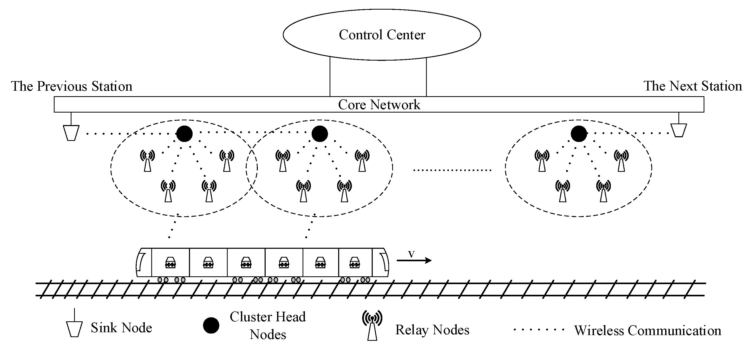
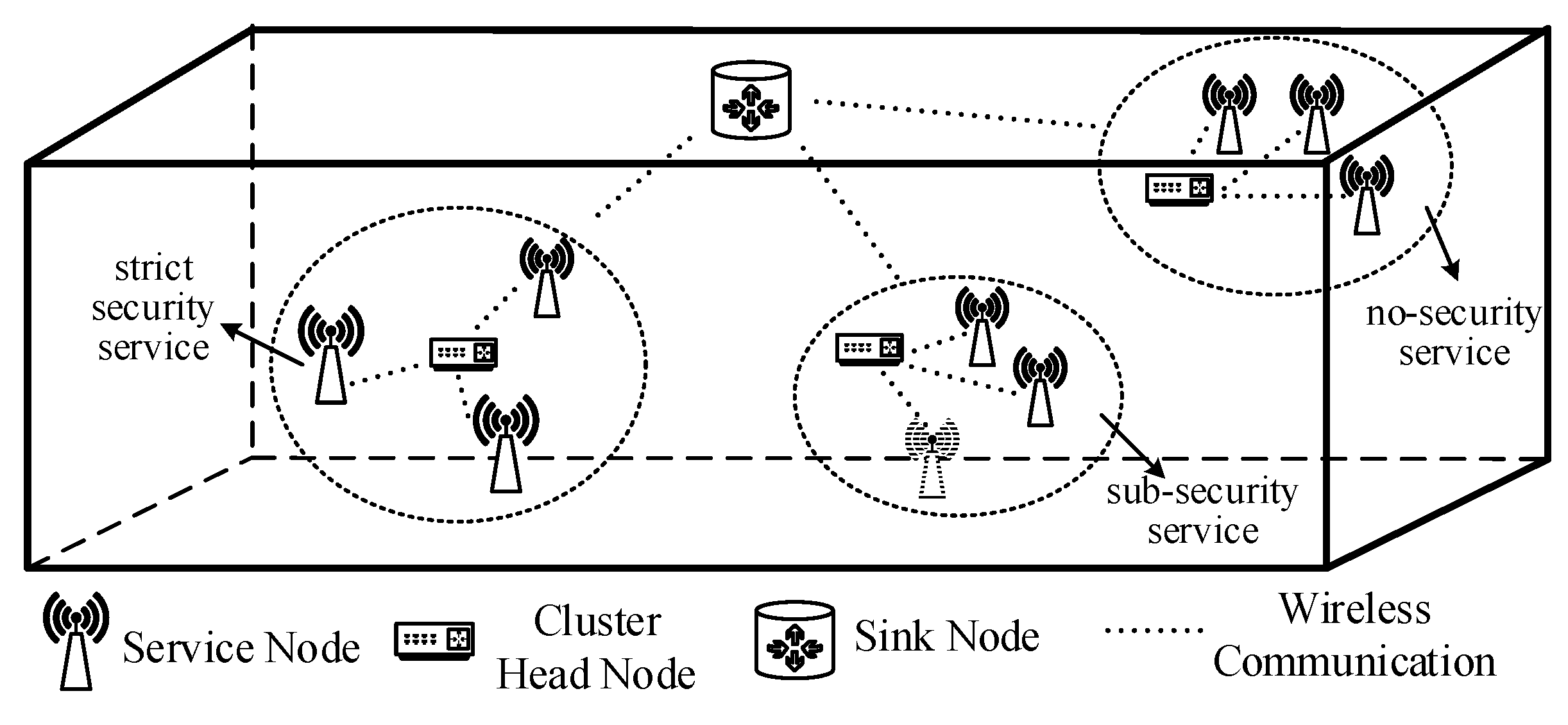
An ad hoc network is a typical decentralized network formed by wireless nodes that can communicate without pre-existing infrastructure. They have been widely used in the internet of things, internet of vehicles, and satellite internet. The train autonomous circumambulate system (TACS) is a development direction of the urban rail transit system, which simplifies the trackside equipment and adopts the intelligent onboard controller as the core, achieving the autonomous and safe operational control of trains [6]. Therefore, it is necessary to utilize the ad hoc network to optimize the vehicle–ground network. By arranging communication nodes reasonably, key areas such as turnouts and curves can be covered, and essential information can be exchanged between each node directly, which realizes the robust and dynamic networking of trains, trackside nodes, and station nodes. Compared with the traditional urban rail communication network, the ad hoc network has the following advantages:

• Decentralized network. Trains and trackside equipment can communicate directly under the ad hoc network without being forwarded by the central nodes;
• Lower cost. Construction and maintenance costs of the base station and the core network can be reduced due to the simplification of the infrastructure, and the cost of deploying cables can also be reduced because of the wireless communication between each trackside node;
• Lower time delay. Direct communication between trains and trackside equipment can reduce the time delay of forwarding;
• Strong network robustness. Because of the cancellation of central nodes, damage to some nodes will not seriously affect the whole network’s performance, leading to the network having strong survivability.

Ad hoc networks can be divided into flat networks and hierarchical clustering networks [7]. Flat networks have a peer-to-peer structure, making it difficult to uniformly manage and maintain each node with the movement of nodes in an extensive network. Therefore, the flat topology results in the easy interruption of network links. In addition, each node under this topology maintains routes to all other nodes, resulting in high overheads and low network scalability.

Under the hierarchical clustering structure, the network is separated into groups called clusters. Each cluster contains one cluster head node and several member nodes. This architecture has two levels: all cluster head nodes constitute the upper-layer network, and normal nodes constitute the lower-layer network. The upper-layer network is responsible for forwarding the data and managing the nodes of the lower-layer network. The clustering structure has the following advantages: (1) Only the cluster heads form the backbone network, rustling in simple topology; (2) Only part of the network is affected when nodes are changed, making the topology more stable; (3) Only the cluster heads need to maintain route information, which reduces the network overhead.

Due to these advantages, researchers have proposed many clustering schemes. Low-energy adaptive clustering hierarchy (LEACH) is a critical and widely considered clustering protocol in ad hoc networks. LEACH chooses the cluster heads based on a random probability number and aims to reduce energy consumption in wireless sensor networks (WSNs). Because the wireless sensor node is battery-powered, an energy-efficient routing protocol should be considered in a WSN to extend network lifetime. Although LEACH has been proposed for a long time, it has also been researched widely in recent years and has good performance. CH-leach is proposed to optimize cluster head selection in ref. [8], which divides clusters by the k-means algorithm, and selects the node nearest to the cluster center as the cluster head. But the algorithm in ref. [8] only has one cluster head for each cluster, which may cause hot-zone problems, and its ability to combat network congestion is weak. To solve the problem, Wang proposed a non-uniform clustering algorithm based on LEACH, which selects double cluster heads to prolong the network lifetime [9]. Furthermore, machine learning algorithms have also been used to select cluster heads. In ref. [10], a genetic algorithm (GA) is utilized for optimal cluster-head selection in the LEACH protocol, which can extend the lifetime to about three times that of conventional LEACH. Another useful machine learning algorithm in these networks is the ant colony optimization algorithm, which can help to find the best route. Authors in ref. [11] used an improved ant colony optimization method to find optimal multi-hop paths according to the residual energy of the next hop node. To avoid unnecessary energy consumption, energy-efficient dynamic and adaptive state-based scheduling (EDASS) was proposed [12], which can dynamically switch nodes between four states of route, active, wait, and sleep, and in this way, highly efficient energy management can be achieved.

In addition to WSN, a vehicular ad hoc network (VANET) is another widely used type of network, which has the characteristics of strong mobility and rapid topology change. QMM-VANET is proposed in ref. [13], which considers quality-of-service (QoS) requirements, the distrust value parameters, and mobility constraints. To reduce the influence of vehicle movement, Luo took into account the location information of vehicles and divided geographical locations into grids for clustering [14]. A wireless body area network (WBAN) is another new ad hoc network which has been developed in recent years. The WBAN is based on the human body and composed of network elements related to the human body. Authors in ref. [15] proposed an efficient QoS-based multi-path routing (MPR) scheme for WBAN, which divided data traffic into normal and emergency types, and the emergency traffic is routed onto the best path.

In an urban rail transit scenario, ad hoc networks have often been used to monitor train operational status and the carriage environment. In ref. [16], a clustering algorithm was utilized to maximize the lifetime of the high-speed railway network under the WSN network. Another cluster algorithm was proposed in ref. [17], which was used to minimize and balance the energy consumption of nodes. However, nodes used for vehicle–ground critical service transmission are powered by cables, so there is no need to save node energy as in a WSN network. In addition, trackside nodes are distributed along tunnel walls, and only the train is moving, which is different from VANET. Therefore, a novel clustering routing protocol is needed to meet the needs of urban rail transit vehicle–ground communication.

In this paper, we adopt an ad hoc network for the urban rail transit system and propose a clustering algorithm based on improved ant colony optimization. The contributions of this paper are as follows:

• An ad hoc network is deployed in an urban rail transit scenario, which can help to improve the robustness of the vehicle–ground network and the driving safety. Furthermore, urban rail transit is different from WSN or VANET, due to the fixed driving environment, power-suppliable nodes, and large data traffic;
• A cluster-head selection strategy based on cost function is proposed to reduce packet loss rate, which can elect cluster head nodes periodically and change cluster head nodes according to the packet loss rate;
• A low-delay queuing strategy based on service priority is proposed to reduce end-to-end delay, which can guarantee the time delay according to different service requirements;
• An improved ant colony algorithm is proposed to find the best route from source node to destination node, which integrates the route length, search direction, and node load to find a path.

The rest of this paper is organized as follows. In Section 2, we introduce the communication network architecture. The proposed algorithm and the network flow are discussed in Section 3. Section 4 shows the simulation results for end-to-end delay, packet loss rate, and throughput, and compares the proposed algorithm with classic LEACH and the ad hoc on-demand distance vector (AODV). Finally, Section 5 concludes the paper.

2. The Network Architecture

2.1. In-Vehicle Network Architecture

Figure 1 shows the network topology in a carriage, and the in-vehicle network includes three types of nodes: service nodes, cluster head nodes, and sink nodes.

1.

Service nodes. Service nodes are responsible for bearing different services. Generally, urban rail transit services can be divided into security and non-security services. Security services are essential for the safe operation of the train, such as the operation control service, video monitoring service, emergency text service, and operating conditions monitoring service. Non-security services generally refer to passenger services with lower latency requirements, such as web browsing, video calls, and online games [18]. In this paper, we classify the services into three priorities according to the delay and reliability requirements: strict security service, sub-security service, and non-security service, as shown in Table 1.

2.

Cluster head nodes. As mentioned above, cluster heads are responsible for forwarding the service data and managing the cluster members, usually selected by a selection algorithm. In this study, we elected cluster heads considering comprehensively the factors affecting the time delay and packet loss rate. In addition, we also set a low-delay queuing strategy for the cluster head nodes. Under this strategy, cluster heads can always forward the high-priority services first.

3.

Sink nodes. Sink nodes are the superior nodes of cluster heads. They are deployed at the carriage’s top center, responsible for receiving data from cluster heads and then forwarding information to the trackside system. In the ad hoc network, each node works according to the method of time-division multiple access (TDMA). The sink nodes are responsible for issuing the schedule to avoid resource collision and network congestion.

Figure 1. In-vehicle network architecture.

Figure 1. In-vehicle network architecture.

Table 1. The categories of urban rail services.

Security Service		Non-Security Service
Strict Security Service	Sub-Security Service
Operation control system (OCS)	Train operation status monitoring (TOSM)	Passenger multimedia service
Operational voice communication system (OVC)	Passenger information service (PIS)
	Closed-circuit television (CCTV)

Table 1. The categories of urban rail services.

Security Service		Non-Security Service
Strict Security Service	Sub-Security Service
Operation control system (OCS)	Train operation status monitoring (TOSM)	Passenger multimedia service
Operational voice communication system (OVC)	Passenger information service (PIS)
	Closed-circuit television (CCTV)

2.2. Vehicle-Ground Networking Architecture

The vehicle–ground network architecture is shown in Figure 2. We assume that the trackside nodes are randomly distributed along the tunnel wall, and the k-means algorithm is utilized to divide clusters. Assuming that the trackside nodes are $x_1,x_2,x_3,\cdots ,x_n$ the clustering process can be divided into the following steps:

• Step 1: Determine the number of clusters, which is denoted as K. Then, randomly select K nodes as the center of each cluster, which are denoted as $u_1^{(0)},u_2^{(0)},u_3^{(0)},\cdots ,u_k^{(0)}$;

• Step 2: Calculate the loss function $J(c,\mu )=\min {\displaystyle \sum _{i=1}^n{‖x_i-{\mu }_{c_i}‖}^2}$, where $c_i$ is the cluster for $x_i$. Then, repeat Step 3 and Step 4 until cluster members do not change with the repetition;

• Step 3: Assign $x_i$ to the cluster with the minimum $J$;

• Step 4: Recalculate cluster central nodes as $u_1^{(1)},u_2^{(1)},u_3^{(1)},\cdots ,u_k^{(1)}$;

In Step 1, we depend on the sum of the square errors and cluster load to determine K, which can be expressed by the following formula:

$$SSE={\displaystyle \sum _{i=1}^k{\displaystyle \sum _{p\in C_f}{\left|p-u_{c_i}\right|}^2}},$$

(1)

$$CL={\displaystyle \sum _{i=1}^{n_{c_i}}{L}_{c_i}},$$

(2)

where $p$ is the cluster member of $c_i$, $L_{c_i}$ is the packet length of $p$. For $K\in [k_1,k_n]$, the value that can minimize the clustering evaluation value is selected as the number of clusters. The clustering evaluation value can be calculated by Equation (3):

$$EV=a_1\ast SSE+a_2\ast CL,$$

(3)

where $a_1$ and $a_2$ are evaluation coefficients. Cluster load is an importance parameter in an urban rail transit scenario, which affects whether the network is congested, and square error is also a valuable evaluation parameter. Based on this, $a_1$ and $a_2$ are set to the same value in this paper. Therefore, we have $a_1=a_2=0.5$.

Similarly, the communication nodes in the vehicle–ground network system include relay nodes, cluster head nodes, and sink nodes.

• Relay nodes. Relay nodes are responsible for forwarding the information from the vehicle to the trackside cluster heads. Unlike in-vehicle service nodes, relay nodes do not carry specific services but only play the role of the wireless relay. Each relay node has equal status and the same communication ability and can participate in cluster-head election.
• Cluster head nodes. Cluster head nodes in the vehicle–ground network have the same function as in the in-vehicle network.
• Sink nodes. In the in-vehicle network, sink nodes are deployed on the top center of the carriage, but in the vehicle–ground network, sink nodes are located at the stations. Sink nodes in the vehicle–ground network are responsible for forwarding the data from cluster heads to the core network. Considering the time delay, when the train is in the first-half area between two stations, the data packets are forwarded to the sink node of the previous station and vice versa to the sink node of the next station.

Figure 2. Vehicle–ground network architecture.

Figure 2. Vehicle–ground network architecture.

3. The Proposed Algorithm

The proposed algorithm in this paper consists of cluster-head election, latency optimization methods, and an improved ant colony optimization method. In this section, the algorithm and the network flow are introduced in detail.

3.1. The Network Flow

The network flow can be divided into seven steps, described in

Table 2. Network flow.

Stage	Function
Step 1: Initial phase	Initialize the network. At this time, all nodes do not belong to any cluster.
Step 2: Flooding phase	All nodes in the network broadcast data packets containing their service type, geographic location, and IP address until each node knows the other nodes’ information.
Step 3: Clustering phase	In-vehicle network: The service nodes with the same service type form a cluster, calculate the cost value based on the method in Section 3.2, and broadcast it in the cluster.
	Vehicle–ground network: Nodes are clustered by the k-means method. Then, the cost value is calculated based on the method in Section 3.2 and broadcasted in the cluster.
Step 4: Cluster-head electing phase	The node with the minimum cost becomes the cluster head. The selected information is broadcasted in the network.
Step 5: Routing phase	The best route is selected according to the improved ACO method in Section 3.4.
Step 6: Working phase	The member nodes and cluster heads start to work. Each cluster head node forwards data according to the method in Section 3.3.
Step 7: Finish phase	When the network finishes a round, restart the network from Step 3.

.

3.2. Cluster-Head Election Strategy Based on Cost Function

Due to the characteristics of decentralization, each node in an ad hoc network can be the cluster head. Therefore, how to select a suitable node to be the cluster head and dynamically update it is a significant problem. A common method is to use multi-factor analysis to jointly evaluate the ability of each node as the cluster head. Based on this, we propose a cluster-head election strategy based on cost function (CHCF).

The algorithm comprehensively considers two variables: distance and packet loss rate. There are two types of distance: the distance between the node and the next hop, as shown in Equation (4), and the distance between the node and the cluster center, as shown in Equation (5). Note that the center node here is a virtual node based on the location information of cluster member nodes.

$$\mathrm{dis}(i)=\sqrt{{\left(x_i-x_{\mathrm{next} }\right)}^2+{\left(y_i-y_{\mathrm{next} }\right)}^2+{\left(z_i-z_{\mathrm{next}}\right)}^2},$$

(4)

$$\mathrm{cen}(i)=\sqrt{{\left(x_i-\frac{1}{N}{\displaystyle \sum _{j=1}^N{x}_j}\right)}^2+{\left(y_i-\frac{1}{N}{\displaystyle \sum _{j=1}^N{y}_j}\right)}^2+{\left(z_i-\frac{1}{N}{\displaystyle \sum _{j=1}^N{z}_j}\right)}^2},$$

(5)

where $\mathrm{dis}(i)$ and $\mathrm{cen}(i)$ are the two separate types of distance. $(x_i,y_i,z_i)$ represents the coordinate of node $i$, $(x_{next},y_{next},z_{next})$ is the coordinate of the next hop node, and $N$ refers to the node number in the cluster.

The packet loss rate is essential for communication reliability. In CHCF, the cluster head is re-elected each time period, which is denoted by $T$. At the end of each round, clusters calculate the average packet loss rate according to the packet number sent by the previous cluster and received by the current cluster head, as shown in Equation (6):

$$loss\_rate=1-\frac{Packet\_receive}{Packet\_send}.$$

(6)

We use the two variables to calculate each node’s cost value, and the node with the minimum cost value is elected as the cluster head. The specific calculation method is as follows:

$$C(i)=\left\{\begin{array}{cc}{k}_1\frac{dis(i)}{{\displaystyle \sum _{j=1}^{n}dis(j)}}+k_2\frac{cen(i)}{{\displaystyle \sum _{j=1}^{n}cen(j)}}& ,loss\_rate\le c_{threshold}\\ 1& ,loss\_rate>c_{threshold}\end{array}\right.,$$

(7)

in which $C(i)$ is the cost value and $k_1$ and $k_2$ are cost factors, which represent the influence level of different variables and have a relationship of $k_1+k_2=1$. In this paper, $k_1$ and $k_2$ are set as 0.5 and 0.5, respectively, considering the two factors are of equal importance. $c_{threshold}$ indicates the threshold of packet loss rate. After each network round, cluster heads compare the value of $loss\_rate$ with $c_{threshold}$. If $loss\_rate>c_{threshold}$, the current cluster head is restored as a common node and is not elected in the next round. If $loss\_rate\le c_{threshold}$, the current cluster head continues to be the cluster head in the next round. In this way, the reliability requirements of urban rail services can be guaranteed.

3.3. Low-Delay Queuing Strategy Based on Service Priority

Reducing the delay of delay-sensitive services in urban rail transit is a significant problem in guaranteeing secure driving. End-to-end delay consists of transmission, propagation, queuing, and processing delays. The propagation delay is related to the propagation distance. In Section 3.1, we use the distance factor when electing cluster heads to reduce the propagation delay. Queuing delay refers to the waiting time for service after packets arrive at the router, which is affected by router processing capacity and network congestion degree. When a data packet arrives at an overloaded node, a sizeable queuing delay is generated, and significantly affects the timely delivery of delay-sensitive services. Therefore, it is necessary to focus on a low-delay queuing strategy to guarantee meeting the delay requirements of different services [19].

This paper proposes a low-delay queuing strategy based on service priority (LDQSP). Assuming that the packet size of the same service and the processing capability of the routers are the same, and the arrival probability of data packets follows the Poisson distribution. The M/G/1 model in queuing theory is utilized to analyze the queuing time.

In traditional networks, data packets adopt the first-come-first-served method, which cannot optimize for service requirements. In LDQSP, data packets wait for packets being processed and packets with higher priority to complete processing before being served. Therefore, high-priority services can always be processed first, which can ensure the requirements of delay-sensitive services are met.

In queuing theory, $\lambda$ refers to the average number of packets arriving at the queuing system per unit of time, and $\mu$ refers to the number of packets a router can process per unit of time. $\rho$ indicates queuing strength, which meets $\rho =\lambda /\mu$. To consider the service priority, we have Equation (8) according to the Pollaczek–Khintchine formula:

$$L_Q=\frac{{\rho }^2}{2(1-\rho )},$$

(8)

in which $L_Q$ is the average queue length. Based on the Little theorem, the average queue time $W_Q$ should be:

$$W_Q=\frac{L_Q}{\lambda }=\frac{\rho R}{1-\rho },$$

(9)

where $R$ is the average remaining time of packets under processing when the current packets arrive. Therefore, the average time in the queue satisfies Equation (10):

$$W_S=W_Q+W_B=\frac{\rho R}{1-\rho }+\frac{1}{\mu },$$

(10)

in which $W_B$ is the average process time for a packet.

Assuming that the service priorities in the network are ranked from high to low as $1, 2, 3, \dots , i, i+1, i+2, \dots , n$, when considering the service priority, the average queuing time of the service with priority $i$ consists of three parts:

• The remaining time of the packet being processed;
• The waiting time of the packets already in the queue with higher priorities;
• The waiting time for newly arrived packets with higher priorities in the waiting process.

Based on the analysis in ref. [20], $W_S(i)$ satisfies:

$$W_S(i)=W_Q(i)+W_B(i)=\frac{{\displaystyle \sum _{j=1}^n{\rho }_j{R}_j}}{(1-{\displaystyle \sum _{j=1}^i{\rho }_i})(1-{\displaystyle \sum _{j=1}^{i-1}{\rho }_i})}+\frac{1}{{\mu }_i}.$$

(11)

Therefore, the end-to-end delay of the service with ith priority is as follows:

$$T_{avg}=W_S{(i)}_1+{\displaystyle \sum _{j=2}^n{W}_S{(i)}_j}+{\displaystyle \sum _{j=1}^n{t}_{trans}{(i)}_j},$$

(12)

where $t_{trans}{(i)}_j$ is the propagation delay of the hop $j$, and $W_S{(i)}_j$ is the average time in the queue of the hop $j$. Note that each cluster of the in-vehicle network is composed of service nodes with the same priority. $W_S{(i)}_1$ and $W_S{(i)}_j$ should be calculated by Equations (10) and (11), respectively.

3.4. The Ant Colony Optimization Method

After completing the cluster-head election, an effective routing algorithm is needed to complete the end-to-end communication from the train to the station. In the routing process, the source node and destination node are train and station, respectively, and the intermediate nodes are cluster heads. As a classical swarm intelligence algorithm, ant colony optimization (ACO) was first proposed in ref. [21], and is usually used to solve the problem of complicated combination optimization. Considering the similarity between finding the best route and ant colony foraging, an improved ACO algorithm is proposed in this section.

ACO uses the pheromone left by ants in foraging to find the optimal path. Pheromone is a substance left by ants on the path in the process of foraging, and ants can sense the pheromone intensity. Therefore, more ants pass along the path with stronger pheromone, and a positive feedback mechanism is formed, thereby gradually approaching the optimal path [22]. In the foraging process, the node with higher pheromone concentration has higher probability of being selected, but ants also choose the next hop based on higher heuristic information. Therefore, the next hop is determined according to the transition probability comprehensively calculated according to the pheromone concentration and heuristic information left on the current node path, which can be described by Equation (13) [21]:

$$p_{ij}^k(t)=\left\{\begin{array}{cc}\frac{{[{\tau }_{ij}(t)]}^{\alpha }{[{\eta }_{ij}(t)]}^{\beta }}{{\displaystyle {\sum }_{u\in J_k(i)}{[{\tau }_{iu}(t)]}^{\alpha }{[{\eta }_{iu}(t)]}^{\beta }}},& j\in J_k(i)\\ 0,& j\notin J_k(i)\end{array}\right.,$$

(13)

where $p_{ij}^k(t)$ is the transition probability of ant $k$ from node $i$ to node $j$ at time $t$, ${\tau }_{ij}(t)$ and ${\eta }_{ij}(t)$ are the pheromone concentration and heuristic information, respectively, $\alpha$ and $\beta$ represent the importance of the pheromone concentration and heuristic information, and $J_k(i)$ indicates the optional node set of ant $k$ at node $i$, which is the set of nodes that have not been visited. Based on Equation (13), ant $k$ determines the next hop node until arriving at the destination node. After all ants arrive at the destination node, the shortest route is saved, and then the pheromone concentration of each route is updated. After a certain number of iterations, all ants tend to choose the same path, and the algorithm reaches convergence.

${\eta }_{ij}(t)$ is usually calculated as $1/d_{ij}(t)$ in traditional ACO, in which $d_{ij}(t)$ is the distance between node $i$ to node $j$ at time $t$. Compared with other ad hoc networks, the urban rail transit scenario has the characteristics of linear distribution and huge data traffic; thus, specifying the routing direction and avoiding node congestion should be considered. In this paper, three factors are considered when calculating ${\eta }_{ij}(t)$, as shown in Equation (14):

$${\eta }_{ij}(t)=a_1\cdot norm[\frac{1}{d_{ij}(t)}]+a_2\cdot norm[\frac{1}{2-\cos {\theta }_{ij,id}(t)}]+a_3\cdot norm[(1-q_j(t))],$$

(14)

in which $norm[\cdot ]$ indicates the normalization operation, $\cos {\theta }_{ij,id}(t)$ indicates the cosine value of the angle between edge $ij$ and edge $id$, where node $d$ represents the destination node. Assume that the train moves from $z_1$ to $z_m$, and the train’s position is $z_t$ at time $t$. Based on the assumption, $q_j(t)$ is the ratio of the number of times node $j$ has been selected as the node on the best path in the process from $z_1$ to $z_t$ and the total path number from $z_1$ to $z_t$. According to Equation (14), ${\eta }_{ij}(t)$ is constrained by $d_{ij}(t)$, $\cos {\theta }_{ij,id}(t)$, and $q_j(t)$, which influence the route length, search direction, and node load, respectively.

${\tau }_{ij}(t)$ is updated at the end of each iteration, according to Equation (15):

$${\tau }_{ij}(t+1)=(1-\rho (t)){\tau }_{ij}(t)+{\displaystyle \sum _{k=1}^m\Delta {\tau }_{ij}^k},$$

(15)

where $\rho (t)$ is the pheromone volatilization factor and $\Delta {\tau }_{ij}^k$ is the pheromone left by ant $k$ on path $ij$. $\rho$ and $\Delta {\tau }_{ij}^k$ are improved by Equations (16) and (17):

$$\rho (t+1)=\rho (t)(1-e^{-t}),$$

(16)

$$\Delta {\tau }_{ij}^k=\frac{Q}{L_{best}}(1-q_j(t)),$$

(17)

in which $Q$ is a constant and $L_{best}$ represents the length of the best route. According to Equation (16), the pheromone volatilization factor gradually increases with the number of iterations, which can increase the search depth and avoid falling into local optimum. Compared with the traditional method Equation (17) adds the node’s load factor and can avoid selecting congested nodes during routing.

4. Simulation Results

This section presents the simulation results for end-to-end delay, packet loss rate, and throughput for the urban rail transit communication network under the proposed protocol. In order to validate the performance of our algorithm, we compare it with the LEACH clustering protocol and AODV routing protocol. LEACH utilizes random numbers to elect cluster heads periodically and AODV is an on-demand routing protocol based on node sequence number, and both are classical algorithms used in ad hoc networks.

4.1. Simulation Parameters

The simulation scenario is a typical tunnel within an urban rail transit system, which begins from one station and ends at the next station. The trackside nodes are randomly distributed along the tunnel wall, and the nodes in the train are also distributed randomly. Source nodes on the trackside are changed as the train moves, and destination nodes are located at the stations. Therefore, we only consider the simulation from the station to the middle of the tunnel, due to the symmetry on both sides of the tunnel.

The transmission power and the receiver sensitivity are set to10 dBm and −77 dBm, respectively. Each transceiver antenna’s gain is 5 dBi, and the frequency point is 2.4 GHz. The parameters above were obtained based on [23]. The parameters of the improved ACO algorithm are also given, which were obtained through a large number of experiments to confirm the best route. The parameters are summarized in

Table 3. Simulation parameters.

Parameter		Value
Parameters of vehicle–ground communication	Carrier frequency	2.4 GHz
	Data rate	20 Mbps
	Transmit power	10 dBm
	Tx Antenna gain	5 dBi
	Rx Antenna gain	5 dBi
	Receiver sensitivity	−77 dBm
Parameters of the improved ACO algorithm	$\alpha ,\beta$	1, 10
	${\alpha }_1,{\alpha }_2,{\alpha }_3$	0.5, 0.3, 0.2
	$Q$	1
	$\rho \left(0\right)$	0.8

.

4.2. Packet Loss Rate Results

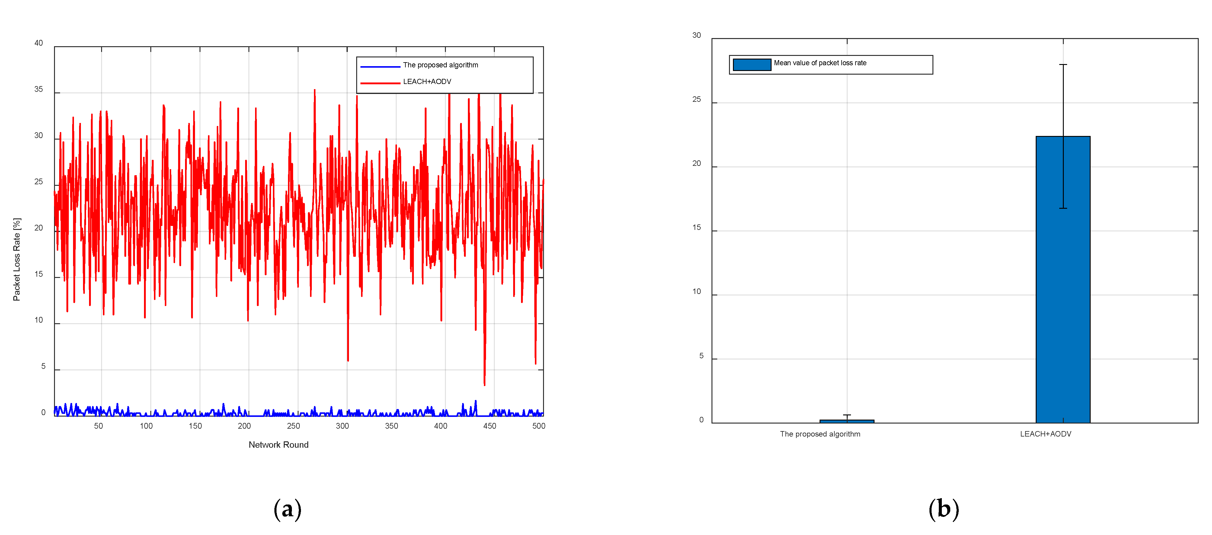
The proposed algorithm utilizes CHCF and the improved ACO algorithm to elect cluster heads and find the best route, and is compared with the LEACH and AODV algorithms. The process was set so that each node had 1000 packets to be sent every round, and the network ran 500 rounds. The statistical packet loss rate results are shown in Figure 3.

Figure 3a shows that the packet loss rate obtained by the proposed algorithm is significantly lower than the packet loss rate obtained by LEACH and AODV, and the error bars of the average packet loss rate are shown in Figure 3b. In Figure 3b, the bars represent the mean value of packet loss rate from network round 1 to round 500, and the vertical line at the top of the bars represents the standard deviation of packet loss rate from network round 1 to round 500. The mean values of packet loss rate are 0.25% and 22.37% for the proposed algorithm and comparison algorithm, respectively. It can be seen from Figure 3b that the proposed algorithm has a smaller and more stable packet loss rate than LEACH and AODV. The reason is that the proposed algorithm comprehensively considers multiple factors to elect cluster heads each round. However, LEACH only elects cluster heads according to a random number in each round, and the node which has been the cluster head cannot continue to serve as the cluster head in the next round. Therefore, the cluster head elected by LEACH can only guarantee the minimum packet loss rate for a short time. In addition, LEACH may elect the nodes at the edge positions to be cluster heads, which leads to the result that the packet loss rate fluctuates widely in different rounds. In contrast, the proposed algorithm re-elects the cluster heads according to the packet loss rate during each round. Thus, a node with a packet loss rate higher than $c_{threshold}$ cannot be the cluster head in the next round. Therefore, the packet loss rate obtained by the proposed algorithm only fluctuates in a small range and always keeps a low value.

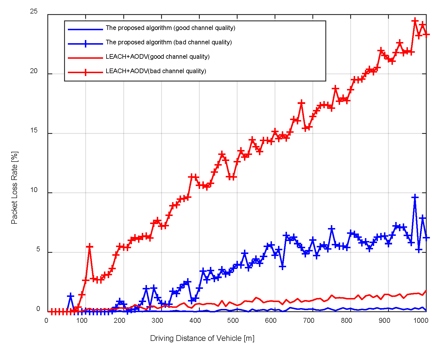
Considering the train is moving and the surrounding environment is constantly changing, it is necessary to validate the performance of the proposed algorithm under circumstances of different channel quality. In Figure 4, we depict the average packet loss when the train is at different positions and obtain the results for different channel qualities. The figure shows that the packet loss rate has an increasing trend, which is because the data packets are sent to the previous station as the train moves on. As the channel quality changes from good to bad, the received signal power decreases, and the packet loss rates of the proposed algorithm and the comparison algorithm both increase. However, the comparison algorithm is affected by channel quality and driving distance more seriously than the proposed algorithm. When the channel quality is bad, the maximum packet loss rate exceeds 20% for LEACH and AODV, while that for the proposed algorithm can still be below 10%. The reason is that as the train moves away from the station, the improved ACO algorithm can always find the best way depending on the shortest distance to neighboring nodes, routing direction, and node loads.

4.3. End-to-End Delay Results

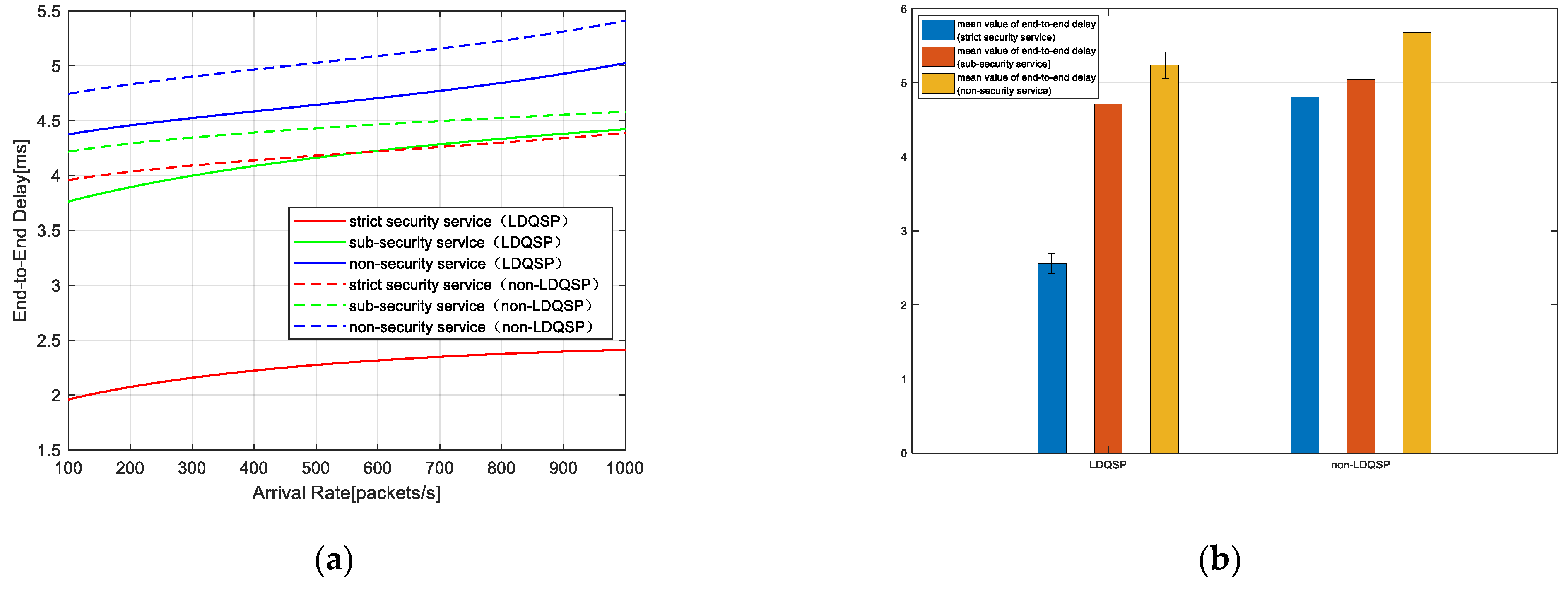
Based on the cluster heads and the best route selected by the proposed algorithm, we compared LDQSP with non-LDQSP in the simulation of end-to-end delay, in which non-LDQSP is a queuing strategy following the principle of first-come-first-served, and the route is found by the improved ACO algorithm.

Figure 5a shows the relationship between end-to-end delay and arrival rate. Since the arrival rate represents the number of packets arriving per time unit, the network becomes more congested with the increase in arrival rate. It can be seen from the figure that as the network becomes congested, the end-to-end delay of all services increases and the delay of LDQSP is lower than that of non-LDQSP. Figure 5b shows the error bars of the mean of end-to-end delay. The bars in Figure 5b represent the mean values of end-to-end delay when the arrival rate gradually increases, and the vertical line at the top of the bars represents the standard deviation of end-to-end delay when the arrival rate gradually increases. It can be seen that LDQSP has less delay than non-LDQSP, especially for strict security safety, which is decreased by about 50% compared with non-LDQSP. The results confirm that our low-delay queuing strategy can significantly guarantee the high-priority services.

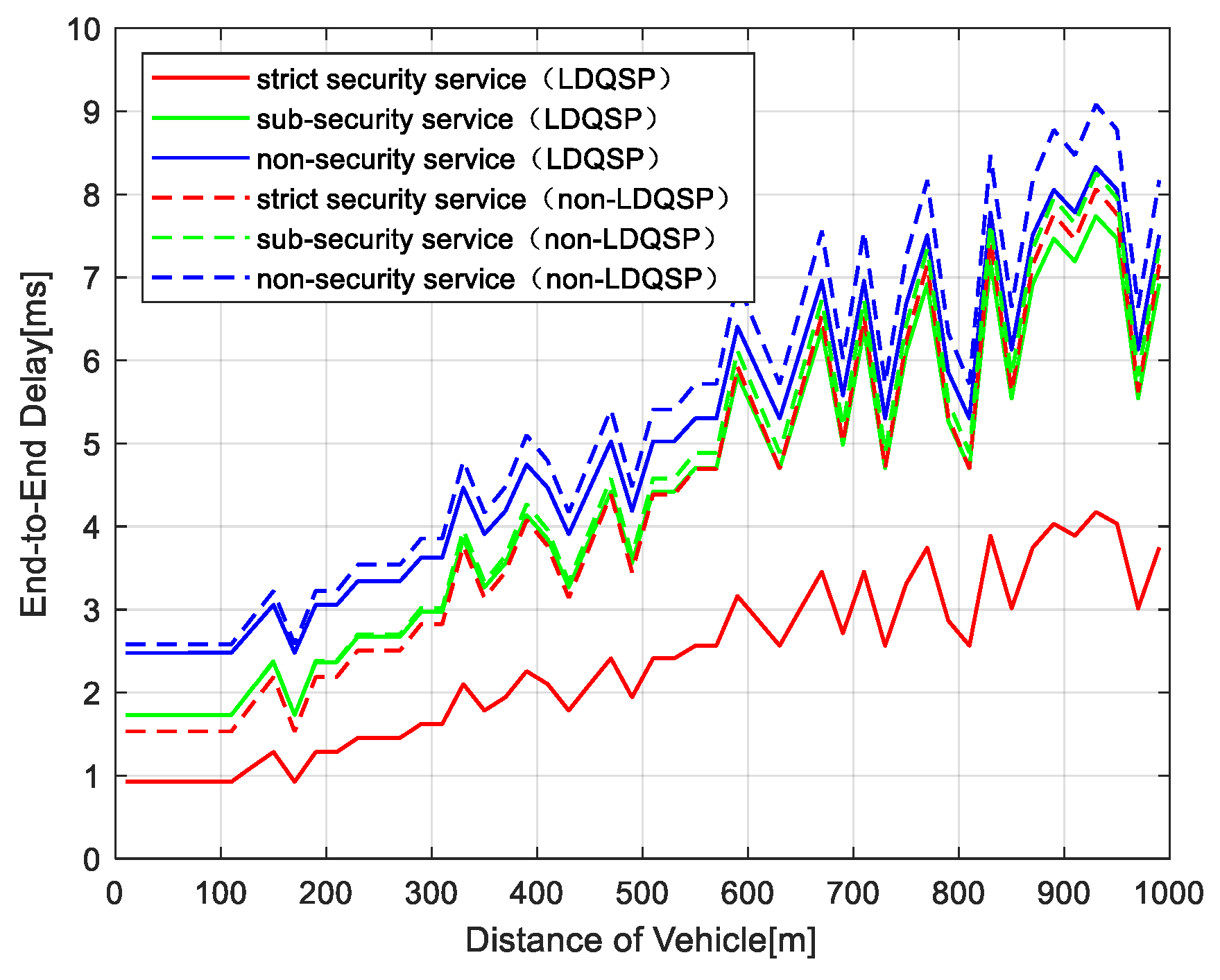
Figure 6 depicts the variation of end-to-end delay with driving distance. Similar to the packet loss rate results, the end-to-end delay also has an increasing trend, which is due to the increase in communication distance and hop numbers as the train moves away from the station. The result of LDQSP is lower than non-LDQSP, which is consistent with the results in Figure 5. Due to the optimization for different services in LDQSP, the delay has less fluctuation than that of non-LDQSP, which ensures the data packets can be delivered to the receiving end in time.

4.4. Throughput Results

The throughput of different services is compared in Figure 7. It can be seen from Figure 7 that the throughput of the proposed algorithm is larger than the throughput of LEACH and AODV, no matter what kind of service. The reason is that the proposed algorithm can achieve lower end-to-end delay and packet loss rate, enabling more data packets to be delivered in a certain time. With the increase in vehicle distance, the throughput gradually decreases, which is because the multiples hops influence the packet-delivery delay and the number of received packets. In addition, by observing the throughput of the three service types, it can be found that the strict security service has the smallest throughput, and the non-security service has the largest throughput, which is appropriate to the services’ characteristics. Non-security services are usually games, video, and other high data-traffic services, and from the simulation of throughput it can be seen that the proposed algorithm can guarantee high throughput.

4.5. Summary

The simulations above compare some key network parameters obtained by the proposed algorithm and the typical algorithms using LEACH and AODV. LEACH and AODV are important algorithms in ad hoc networks and have been widely used in recent years. But the urban rail transit scenario is different from the traditional ad hoc network, due to the linear deployment of nodes and there being no need to consider energy consumption, and to our knowledge there are few works focused on the ad hoc network routing algorithm in this scenario. It can be seen that in an urban rail transit scenario, the proposed algorithm has better performance in terms of packet loss rate, end-to-end delay, and throughput. In addition, the proposed algorithm can guarantee different service requirements according to the service characteristics in urban rail transit, such as reduced delay and packet loss rate for strict security services, greater throughput for non-security services, and better anti-congestion capability. Overall, the proposed algorithm is suitable for the urban rail transit scenario, and can provide better performance than other typical algorithms.

5. Conclusions

In this paper, a clustering algorithm based on an improved ant colony optimization algorithm is proposed, which can meet the communication requirements of next-generation urban rail transit systems with low delay and high reliability. The proposed algorithm includes the cluster-head election algorithm CHCF, low-delay queuing algorithm LDQSP, and a routing method based on improved ACO. CHCF elects cluster heads according to node cost. LDQSP enables cluster heads to implement different queuing strategies according to service priorities to ensure the end-to-end delay requirements of higher-priority services are met. Then, the improved ACO algorithm is used to find the best route under conditions of different train locations and wireless channel quality. Finally, the proposed algorithm was compared with the LEACH and AODV algorithms through simulation. The simulation results indicate that compared with the typical ad hoc network routing algorithms, the proposed algorithm in this paper can guarantee the different services’ requirements, reduce the packet loss rate and end-to-end delay about by 60% and 50%, respectively, and improve the network throughput by about 40% in an urban rail transit scenario.