Abstract
Automated machine learning (AutoML), which aims to facilitate the design and optimization of machine-learning models with reduced human effort and expertise, is a research field with significant potential to drive the development of artificial intelligence in science and industry. However, AutoML also poses challenges due to its resource and energy consumption and environmental impact, aspects that have often been overlooked. This paper predominantly centers on the sustainability implications arising from computational processes within the realm of AutoML. Within this study, a proof of concept has been conducted using the widely adopted Scikit-learn library. Energy efficiency metrics have been employed to fine-tune hyperparameters in both Bayesian and random search strategies, with the goal of enhancing the environmental footprint. These findings suggest that AutoML can be rendered more sustainable by thoughtfully considering the energy efficiency of computational processes. The obtained results from the experimentation are promising and align with the framework of Green AI, a paradigm aiming to enhance the ecological footprint of the entire AutoML process. The most suitable proposal for the studied problem, guided by the proposed metrics, has been identified, with potential generalizability to other analogous problems.
1. Introduction
With the exponential growth of machine learning (ML) and computing power, it has become a hot topic both in industry and the academic world [1]. In response to this burgeoning interest, the automation of machine learning is enabling the construction of models of acceptable quality for tasks such as data processing, exploration of various machine-learning algorithms, and efficient hyperparameter tuning. Therefore, continuous efforts are needed to further advance automation within the domain of machine learning [2]. In this context, ML is a powerful and versatile tool for solving complex problems in various domains. However, ML systems often require a large amount of computational resources, which can have a negative impact on the environment and the energy efficiency of the devices.
Automated Machine Learning (AutoML) is a promising research area that aims to reduce the human effort and expertise required to design and optimize machine learning models [3,4,5]. Nonetheless, AutoML systems often consume a large amount of computational resources and energy, which may have negative environmental and economic impacts [6,7,8].
In this paper, we propose a proof of concept for developing automated machine-learning systems that adhere to the principles of green computing. A proof of concept (PoC) is a partial or incomplete implementation of a method or idea conducted to verify the feasibility of a practical application. It demonstrates that a concept or theory is feasible for useful implementation, helping to mitigate risks, demonstrate value, and optimize performance before full implementation. With this approach in mind, we identify the main challenges and opportunities for integrating green computing techniques into the ML pipeline, such as data preprocessing, model selection, hyperparameter tuning, and deployment. We also discuss some potential applications and benefits of green machine-learning systems for different domains, such as healthcare, education, and smart cities. To conclude this introduction, we outline some open research directions and future perspectives for this novel and promising area of research [9,10].
Although artificial intelligence (AI) and AutoML are known for their potential to contribute to sustainability, the sustainability of AI and AutoML has not received the same level of attention. Building upon this premise, the concept of Green AI was introduced by Schwartz et al. [11] and is an emerging field that focuses on the development of AI algorithms and implementations that are more resource-efficient. This is important because AI has a significant environmental impact, as it requires a large amount of energy to train and run models.
In [12,13,14,15], the carbon footprint of AI computing has been characterized by examining the model development cycle across industry-scale machine-learning use cases while also considering the life cycle of system hardware. This comprehensive perspective underscores the need for further investigation into the sustainability of AI, particularly in terms of economic, social, and environmental aspects.
It is necessary to emphasize the importance of thoroughly assessing our ecological impact and actively avoiding unnecessary and extensive carbon footprints, firmly anchoring our proposals within the realm of sustainability. At the core of our proposal is the integration of Green AI metrics or accurate measurements of energy consumption into the intricate algorithms of AutoML. By incorporating these pivotal metrics, we chart an innovative path toward significantly reducing the inherent carbon emissions in machine-learning processes. This strategic alignment of AutoML with Green AI culminates in a collective stride towards a more environmentally conscious future.
The field of AutoML is inherently complex and not readily amenable to theoretical analysis, thus making empirical research contributions predominant. This necessitates conducting extensive experimental studies, which consume a substantial amount of computational resources and subsequently result in considerable carbon emissions. To mitigate these environmental impacts, it becomes imperative to devise techniques that exhibit higher resource efficiency and enable more rapid evaluations, consequently discarding approaches with subpar performance.
The major proportion of energy consumption and carbon emissions originates from the AutoML process, involving pipeline evaluations and the storage of intermediate search results. However, when formulating an AutoML proposal, it is crucial to adopt a holistic perspective considering the entire lifecycle, which includes data generation, storage, computational efforts, memory requirements during development, and the final benchmarking. It is essential not to judge research initiatives with a significant environmental footprint without carefully evaluating their cost-benefit trade-offs. This paper primarily centers on the AutoML process, aligning with the principle of Pareto, also known as the 80–20 rule and the law of the vital few [16].
The analysis of resource consumption in the context of AutoML is an essential aspect for evaluating the environmental sustainability of automated machine-learning approaches and contributes to the quest for more eco-friendly solutions in the field of artificial intelligence.
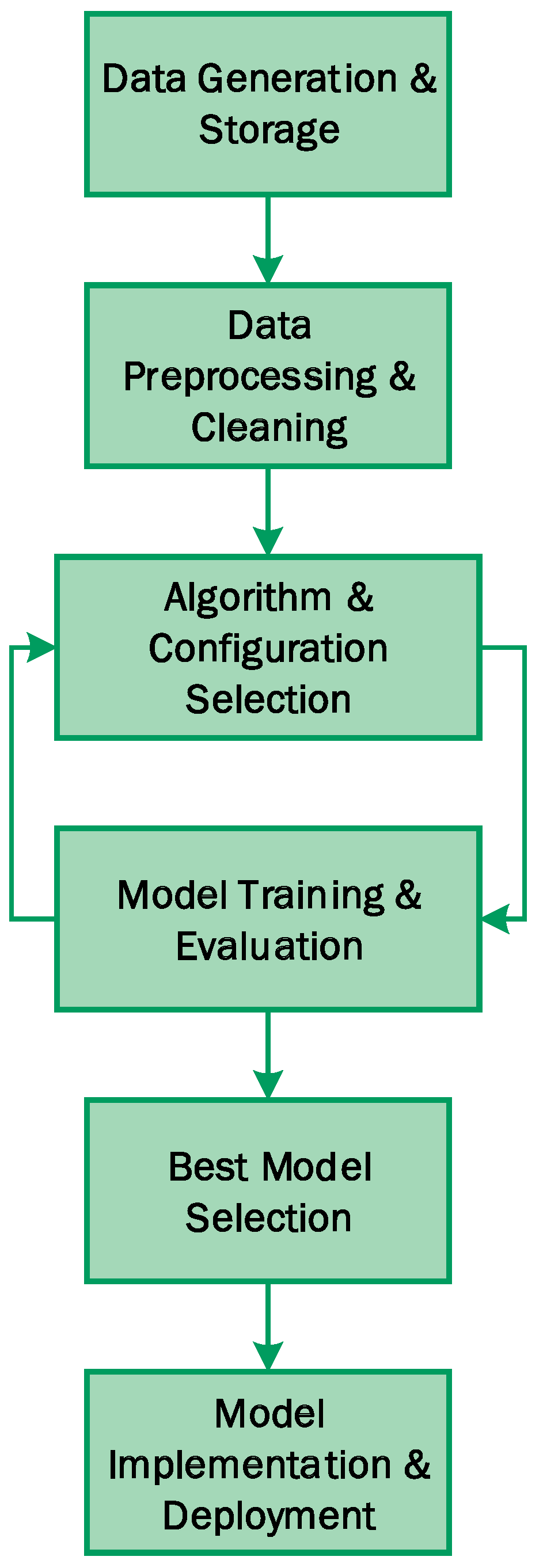
Various strategies have been developed to assess environmental sustainability in the context of AutoML, aiming to identify areas of higher environmental impact and achieve greater optimization for sustainability. Among the most relevant ones are the measurement of computational resource consumption, estimation of carbon emissions, evaluation of energy efficiency, scalability, and analysis of the AutoML lifecycle (Figure 1). Additionally, the performance and quality of models generated by AutoML are compared with the computational effort required. It is also suggested to conduct a comparison of environmental sustainability with traditional manual approaches to understand the environmental advantages of automation in artificial intelligence.
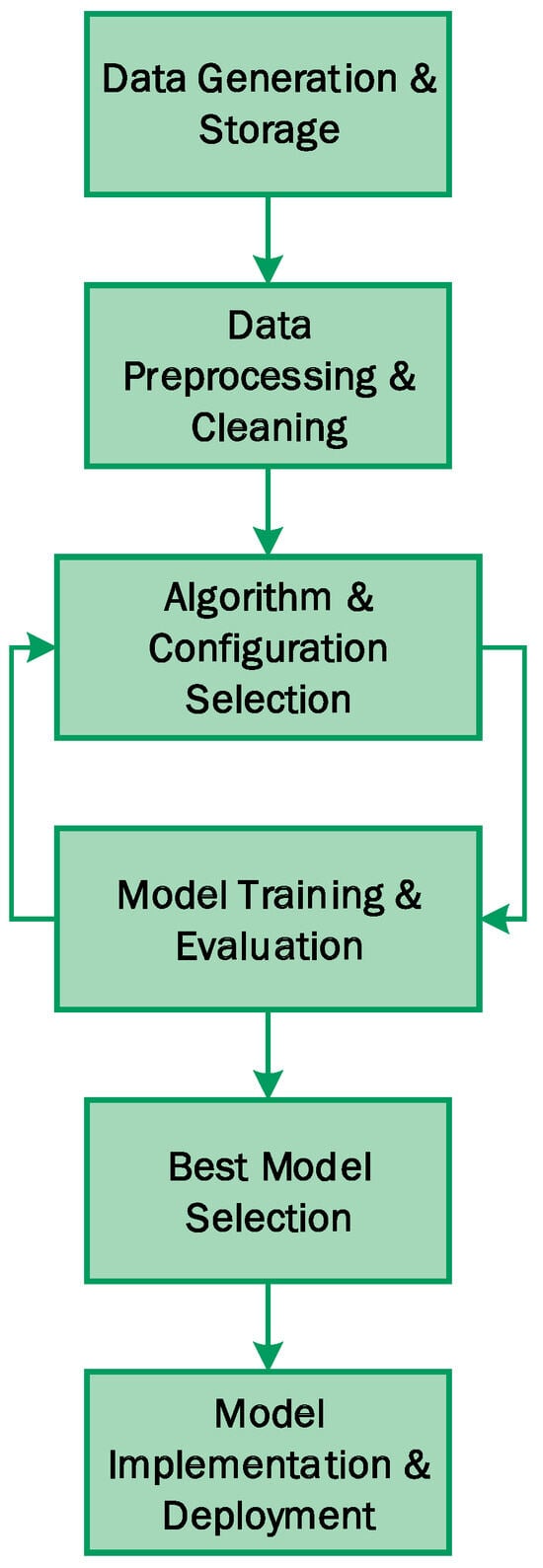
Figure 1.
Illustrates the AutoML lifecycle, encompassing data generation and storage, algorithm and configuration selection, model training and evaluation, and model implementation. Notably, it features a feedback loop that cycles back to the selection of algorithms and configurations after the model training and evaluation stage.
AutoML should not be quantified solely based on the efficiency of an approach or the environmental impact of a specific experiment. Instead, both factors should be considered jointly as research continues to explore the intersection of efficiency and environmental impact [17,18].
A burgeoning solution to the challenge of energy-intensive algorithms is green or sustainable AI [19,20,21,22], which underscores the growing pursuit of ecologically mindful practices within the realm of AI and AutoML. Key strategies include precision–energy trade-offs, energy-aware neural architecture search, model compression, and multi-objective Pareto optimization considering accuracy, latency, and power [23]. Cross-domain transfer learning can also improve sample efficiency and lower training costs [24]. Overall, research toward responsible and eco-conscious AI is rapidly gaining traction. The integration of Green AI principles into hyperparameter optimization and AutoML offers significant potential to mitigate the environmental footprint of developing performant ML solutions.
The objective of this research is to explore the sustainability implications associated with the computational processes within the domain of Automated Machine Learning. In this paper, we have made the following contributions:
- The best hyperparameter optimization strategy was identified using Green AI criteria among frequently used algorithms: Bayesian search and random search in scikit-learn.
- A proof of concept is presented under a Green AI paradigm for the entire AutoML process.
- An experimentation process was implemented based on the principles of Green AI sustainability, which confirmed the validity of sustainability applied to experimentation in AutoML.
The structure of this article is outlined as follows: In Section 2, we provide a review of relevant literature. Section 3 discusses necessary formalizations. The methodology of our proposal is presented in Section 4. The results of this experimentation are detailed in Section 5. Section 6 offers an in-depth discussion of the obtained results. Finally, in Section 7, we present our conclusions and outline directions for future research.
2. State of the Art
The widespread adoption of artificial intelligence (AI) has amplified the importance of achieving a delicate equilibrium between machine-learning model performance and sustainability. Building upon these principles, this is primarily due to the undeniable impact AI systems now exert on our carbon footprint [25,26]. Coping with this challenge has prompted the exploration of diverse strategies.
In the pursuit of this equilibrium, these encompass the curation of more efficient models [27], the meticulous optimization of hyperparameters [28], and the judicious utilization of knowledge transfer [29]. Additionally, the incorporation of reinforcement learning techniques [30], real-time monitoring mechanisms [31], and energy-efficient hardware [32] has emerged as a common practice.
Within this multifaceted landscape, particular attention has been dedicated to life cycle assessments [33] and the design of efficient datasets [34]. In a complementary vein, these facets have been accentuated, recognizing the pivotal roles that awareness and education play in the promotion of sustainability within the machine-learning domain [11].
Hyperparameter optimization for machine-learning algorithms has been a hub of active research, notably witnessing substantial progress in recent works [35,36,37,38]. In response to the growing need for environmentally friendly AI, various optimization strategies have arisen [22,39,40]. These strategies align with Green AI principles and strive to mitigate the environmental repercussions associated with AI development.
Among the most resource-efficient optimization techniques are those based on Bayesian sequential models and their derivatives [41,42,43]. Specifically, they aim to minimize the number of objective function evaluations, thus reducing computational expenses. Bayesian optimization, in particular, leverages probabilistic surrogate models to guide the selection of hyperparameters to evaluate based on prior results [44].
Although most current research centers on carbon footprint monitoring, hyperparameter fine-tuning, and model benchmarking [39], other innovative approaches have sought to reduce the number of iterations needed to find optimal hyperparameters. These strategies, such as those outlined by Stamoulis et al. [45], represent a significant departure from traditional hyperparameter tuning and can substantially diminish the energy costs associated with searching for the optimal set of hyperparameters. Notably, De et al. [46] demonstrated how hyperparameter tuning, when inclusive of energy consumption considerations, can foster the development of more energy-efficient models.
Variational Autoencoders (VAEs) have garnered significant attention due to their potential for crafting compact and lightweight neural networks while incurring minimal loss in accuracy [47]. The utilization of VAEs enables model compression, therefore reducing computational demands and energy consumption [48]. Moreover, VAEs excel in transferring knowledge from extensive teacher networks to more economical student models [29,49]. In a recent study by Asperti et al. [50], a comparative evaluation of various VAE variations was conducted, with a specific emphasis on analyzing the energy efficiency of different models. This research aligns with the principles of Green AI, highlighting the need for enhanced metrics beyond FLOPs (floating-point operations per second) and improved calculation methodologies.
Regarding deep learning models, such as VAEs and Convolutional Variational Autoencoders (ConvVAEs), it is possible to observe slightly divergent outcomes. These variations can be attributed to several contributing factors, as discussed in Sonderby et al. [51]. In the context of ConvVAEs, these outcomes are influenced by factors such as weight initialization, network architecture, and training hyperparameters. These considerations underscore the critical importance of precise configuration and hyperparameter optimization [42]. Additional sources of variation arise from random initialization and dataset diversity, which can impact the learned model parameters and filter responses [52]. In practical terms, the primary objective is to ensure that, despite the inherent variability introduced by these factors, the models effectively capture salient features and maintain consistent performance.
A significant area of uncertainty revolves around whether different training methodologies consistently yield VAEs or ConvVAEs models with similar generative capabilities. It is plausible that divergent training processes result in models with distinct filter weight configurations, while these models continue to exhibit comparable performance [52]. Furthermore, these training processes may potentially yield models with differing architectural configurations, involving variations in the number and type of network layers [53]. Consequently, the performance of these models may diverge, especially concerning the complexity of the data they aim to generate [54]. Clearly, these variations in model architectures bear significant implications for ecological sustainability and significantly influence the development of a sustainable paradigm for artificial intelligence.
Multi-objective optimization techniques, as surveyed by Morales et al. [55] and explored by Kim et al. [56] in the NEMO framework, offer a promising avenue for explicitly integrating sustainability objectives into the model training process. Specifically, these methods employ evolutionary algorithms to Pareto-optimize models for multiple objectives simultaneously, such as accuracy, latency, and energy efficiency.
In a parallel approach, hybrid human-AI approaches, as exemplified by the work of Wilson et al. [57], harness human inputs to enhance model efficiency. In particular, these approaches harness human inputs to enhance model efficiency through human-in-the-loop training. This strategy guides autoencoders toward meaningful and resource-efficient representations, mitigating the computational overhead associated with training. The integration of human domain knowledge further contributes to avoiding the inefficiencies inherent in pure black-box training strategies.
Quantization, as introduced by Zoph et al. [58], emerges as a potent tool for curtailing computational and environmental costs associated with machine-learning models. Essentially, by reducing the number of bits used to represent model parameters and weights, quantization substantially diminishes both model size and energy consumption.
Pruning, elucidated by Han et al. [59], offers another avenue for enhancing efficiency. This involves the removal of unnecessary connections and parameters from a model, leading to reductions in both model size and computational demands.
Lastly, knowledge distillation, originally proposed by Hinton et al. [60] and further advanced by Yang et al. [61], involves the transfer of knowledge from a large teacher network into a smaller student network. This process not only minimizes model complexity but also enhances the sustainability of machine-learning systems by reducing computational demands.
Collectively, the pursuit of sustainable machine learning involves a comprehensive array of strategies spanning efficient model design, hyperparameter optimization, lightweight models, multi-objective optimization, and hybrid human-AI approaches. These strategies form a cohesive approach to not only improving the environmental sustainability of AI but also maintaining and even enhancing model performance.
Overall, promising strides are being made towards sustainable AI. The research discussed in this section highlights some of the most promising approaches to balancing machine-learning performance with sustainability considerations. These solutions encompass a diverse range of methodologies, primarily deployed within the domain of deep learning. In contrast, our proposition centers on tabular data and AutoML solutions utilizing conventional algorithms. This focal point enables the creation of innovative features customized for widely adopted libraries, thus making a meaningful contribution to the sphere of Green AI within the corporate landscape.
3. Bayesian Optimization for Hyperparameter Optimization
In this section, the Bayesian optimization algorithm is examined, as it represents the primary method employed in experimentation. The definition of Bayesian optimization and the hyperparameter optimization problem are both provided.
3.1. Definitions
The hyperparameter optimization problem in machine learning involves finding the optimal set of hyperparameter values for a model that maximizes its performance on a given evaluation dataset. The problem can be formalized as a mathematical optimization problem as follows:
Given a hyperparameter space , an objective function , and a set of constraints , the hyperparameter optimization problem is to find the optimal hyperparameter configuration that either maximizes or minimizes the objective function subject to the constraints .
Here is a breakdown of the formalization:
- is a vector of hyperparameters that configure a machine-learning model.
- is the objective function that measures the model’s performance on an evaluation dataset using a specific metric, such as accuracy, mean squared error, or area under the ROC curve.
- represents the constraints, which can include limitations on allowable values for hyperparameters, constraints on computational resources (such as maximum runtime or available memory), or any other relevant constraints for the problem.
The aim is to find such that:
subject to:
In other words, we want to find the hyperparameter configuration that maximizes the objective function while satisfying all the constraints .
3.2. Bayesian Optimization
In recent years, there has been a growing interest in using Bayesian optimization for hyperparameter optimization. Bayesian optimization is a sequential model-based optimization algorithm that learns a probabilistic model of the objective function and uses this model to guide its search for the optimal hyperparameter configuration . The Bayesian optimization algorithm can be formalized as follows:
- Initialize: Start with a prior distribution over the hyperparameter space .
- Evaluate: Evaluate the objective function at a new hyperparameter configuration .
- Update: Update the prior distribution using the information from the objective function evaluation.
- Select: Select the next hyperparameter configuration using an acquisition function.
- Repeat: Repeat steps 2–4 until a stopping criterion is met.
The acquisition function is a function that measures the expected improvement in the objective function from evaluating the objective function at a new hyperparameter configuration .
A frequently used acquisition function is the expected improvement (EI) function, which is defined as follows:
where is the objective function evaluated at .
The Bayesian optimization algorithm can be used to find the optimal hyperparameter configuration for a wide range of machine-learning models (see Algorithm 1). The algorithm is particularly effective for problems with many hyperparameters, as it can efficiently explore the hyperparameter space.
| Algorithm 1 Bayesian optimization. |
|
In this algorithm, the following variables are utilized:
- is the prior distribution over the hyperparameter space .
- is the objective function.
- is the expected improvement acquisition function.
- and are the mean and covariance of the prior distribution .
- ∣ is the posterior distribution over the hyperparameter space given the objective function evaluation .
4. Materials and Methods
In this section, we describe the methodology used to conduct the research in the context of AutoML experimentation, specifically in relation to Green AI. We present the experimental design, the implementation of algorithms and pipelines, as well as the metrics used to measure energy efficiency and sustainability.
The proposed methodology encompasses the subsequent phases:
- Dataset Selection. The selection of a well-established dataset with minimal storage and processing demands.
- Algorithm and Pipeline Selection. The selection of hyperparameter optimization algorithms, pipelines, and machine-learning algorithms from the proposed AutoML lifecycle.
- Sustainability Metrics Identification. The identification of metrics for evaluating sustainability.
- PoC AutoML Implementation. The implementation of a quantifiably carbon-footprinted proof-of-concept AutoML, utilizing the elements from the aforementioned phases.
- Proposal Evaluation. The comprehensive evaluation of the proposal.
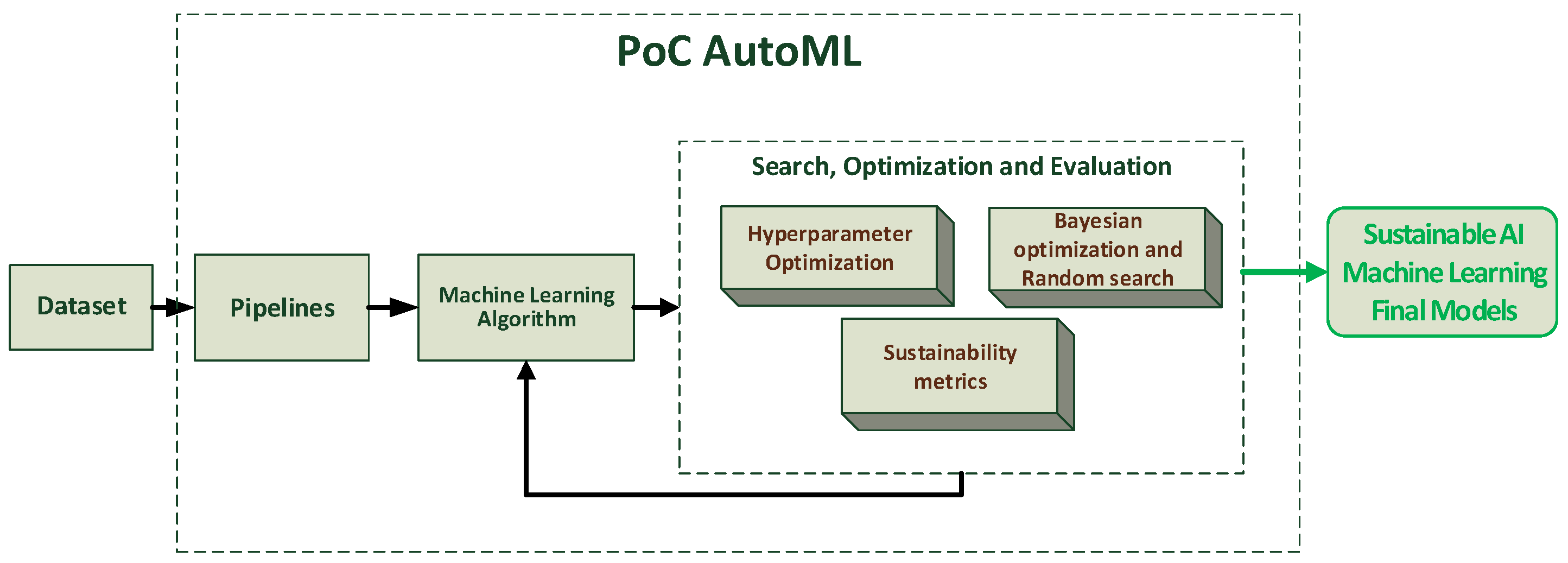
Figure 2 presents a workflow depicting the outlined methodology.
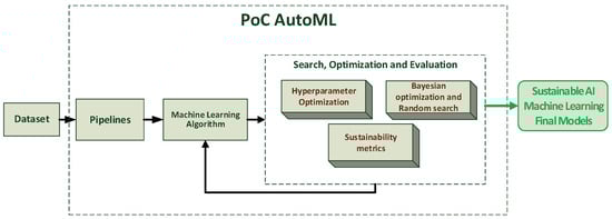
Figure 2.
The illustration shows a workflow of the proposed methodology. It includes the input dataset, the selection of ML algorithms, the search and optimization of hyperparameters with sustainability metrics, the evaluation of the models, and the final model, which is slightly greener AI.
This methodology enables the construction of a more resource-efficient AutoML, which contributes to reducing the environmental impact of artificial intelligence.
4.1. Dataset
For the AutoML experimentation, we selected a dataset widely recognized and extensively used within the machine-learning community. The Breast Cancer Wisconsin (Diagnostic) Dataset [62] was used as the dataset. This dataset serves as a robust and comparative foundation for evaluating diverse AutoML approaches in relation to sustainability and efficiency.
4.2. Proof of Concept on Sustainability within AutoML
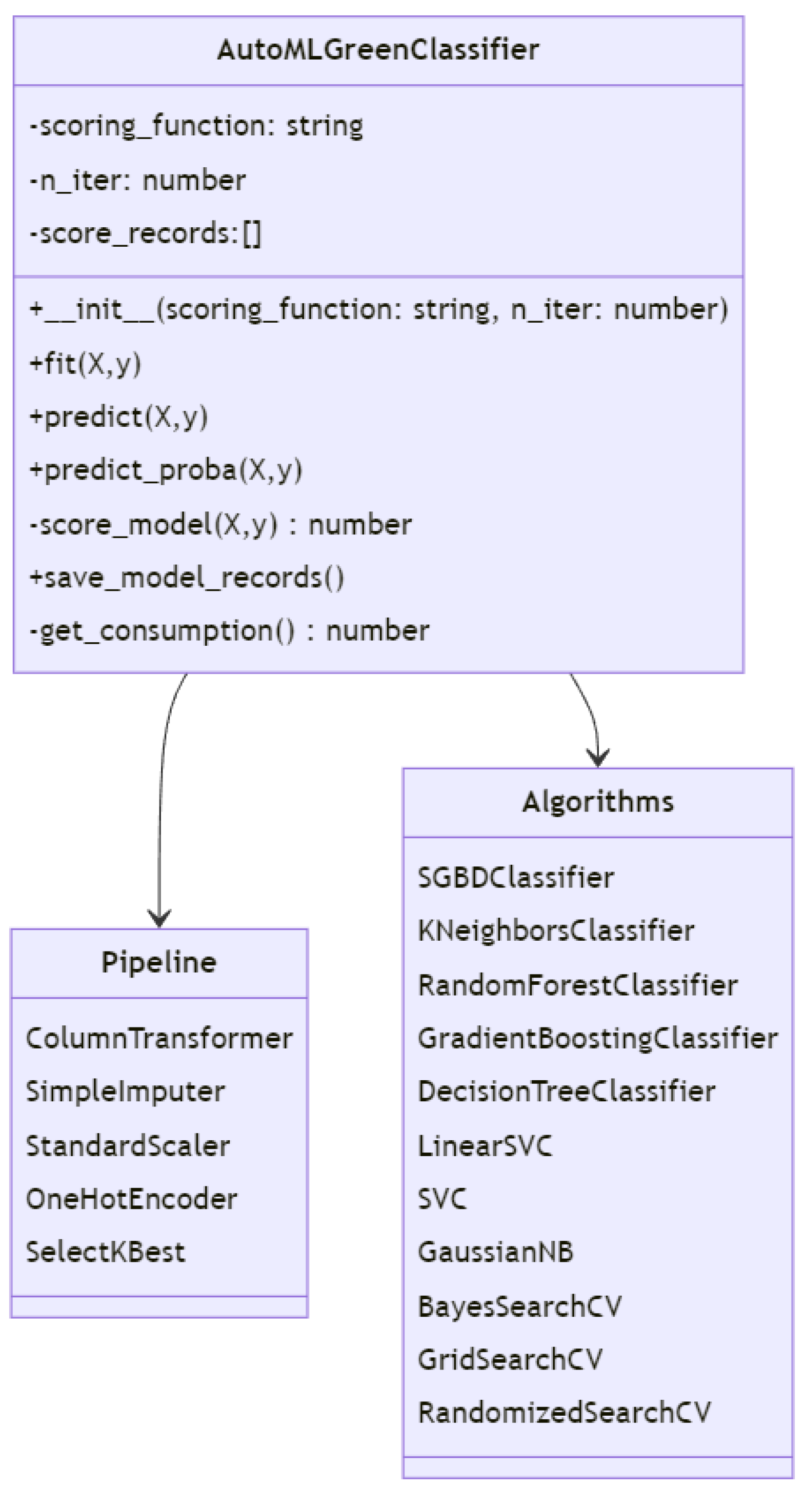
A proof-of-concept study with a specific emphasis on sustainability within the realm of AutoML was undertaken. We established an experimental framework aimed at assessing the influence of various hyperparameter optimization approaches on sustainability, encompassing variables such as training duration, utilization of computational resources, and the corresponding carbon emissions. Figure 3 illustrates the class diagram that presents the primary classes and relationships within a sustainability-oriented AutoML system.
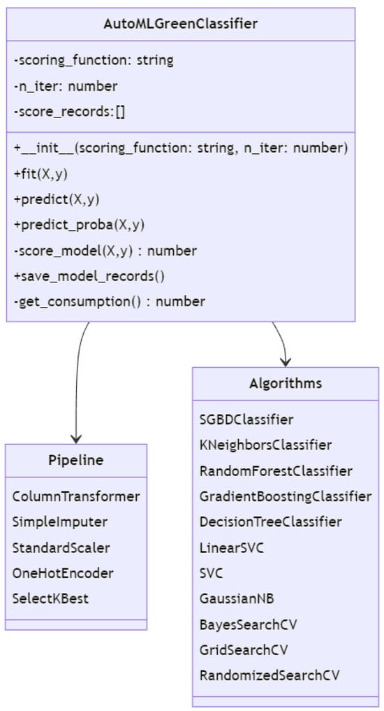
Figure 3.
This class diagram shows the main classes and relationships within a sustainable-focused AutoML system, including the AutoML classifier, data processing pipelines, and a variety of machine-learning algorithms.
4.3. Hyperparameter Optimization, Pipelines, and Machine-Learning Algorithms
Two hyperparameter optimization algorithms were defined: Bayesian optimization (see Algorithm 2) and random search (see Algorithm 3). These selections were made based on their widespread use within the AutoML community and their potential to improve efficiency and sustainability. Grip search was not included as it is computationally very costly and, therefore, has a greater impact on the carbon footprint. Several data preprocessing pipelines and a taxonomy of machine-learning algorithms were designed, covering different approaches and strategies (see Table 1). This allowed exploring a variety of configurations and modeling options, contributing to a comprehensive assessment of sustainability and efficiency.
| Algorithm 2 Bayesian Optimization. |
|

Table 1.
Taxonomy of Machine-Learning Algorithms.
| Algorithm 3 Random Hyperparameter Search. |
|
4.4. Sustainability Metrics
This paper focuses on sustainability aspects induced by computing, as proposed by [63,64,65,66]. These measurements focus on estimating the time and resource consumption, which allows us to determine the carbon footprint of the experimentation in an estimated but precise way. The main metrics identified in the state of the art are [17,25,67,68,69]:
- Runtime is a measure of the time it takes for a program to complete. It is not a perfect measure of efficiency, but it is strongly correlated with the power consumption of the corresponding experiment. Runtime can be used to calculate an estimate of the total carbon footprint of the experiment, but additional information is needed, such as the power consumption of the hardware used and the composition of the power mix. Compared to other measures, runtime is easy to measure on most hardware.
- CPU/GPU Hours. Measuring CPU/GPU hours is a practical and straightforward method for quantifying environmental impact. However, its measurement can be ambiguous, as it can be based on either the actual clock time of CPU/GPU or the real time of CPU/GPU, resulting in different interpretations for quantifying environmental impact. Counting CPU/GPU hours is a suboptimal indicator of efficiency, given its hardware dependence. Nonetheless, it remains one of the most practical metrics due to its ease of measurement and relatively straightforward determination of carbon footprint, assuming that the CPU/GPU consistently consumes a certain amount of energy and that the energy mix is known. The total energy consumption of all active CPU devices (kWh) is calculated as a product of the power consumption of the CPU devices and its loading time , where is equivalent CPU model specific power consumption at long-term loading (kW), is the total loading of all processors (fraction). If the tracker cannot match any CPU device, the CPU power consumption is set to a constant value equal to 100 W [70,71].
- RAM. Dynamic random access memory devices are an important source of energy consumption in modern computing systems, especially when a significant amount of data should be allocated or processed. However, accounting of RAM energy consumption is problematic as its power consumption is strongly dependent on whether data are read, written, or maintained. In RAM, power consumption is considered proportional to the amount of allocated power by the current running process calculated as follows: , where -power consumption of all allocated RAM (kWh), is allocated memory (GB) measured via psutiland 0.375 W/Gb is estimated specific energy consumption of DDR3, DDR4 modules [70,71].
- Energy consumption is hardware-dependent, as it heavily relies on the energy efficiency of the hardware itself. Therefore, while it is a suboptimal metric for assessing the efficiency of a given approach, it proves to be a commendable measure for quantifying the environmental impact of a specific experiment on particular hardware. Notably, energy, in conjunction with the hardware, constitutes the primary external resource required for executing AutoML experiments. Starting from the quantified energy consumption, it is frequently plausible to reasonably approximate the actual carbon dioxide equivalent (CO2e) emissions engendered by the experiment at its specific execution locale and time, given a sufficiency of supplemental information.
- Carbon dioxide equivalent (CO2e) is an excellent and arguably the most direct measure for quantifying the environmental footprint of an experiment, given the provision of the specific physical location and time of execution. However, CO2e, despite its merit, encounters measurement issues that are similar to, or even more complex than, those of energy consumption due to its indirect measurability. The CO2e value as an AI carbon footprint (kg) generated during models learning is defined by multiplication of total power consumption from CPU, GPU and RAM by emission intensity coefficient (kg/kWh) and coefficient: Here, is the power usage effectiveness of the data center required if the learning process is run on the cloud. PUE is the optional parameter with default value = 1 [71]. Rather, it is calculated based on energy consumption coupled with supplementary information concerning the energy mix. In practical terms, procuring corresponding information frequently proves unfeasible, with even the energy mix susceptible to variation depending on external influences, such as climatic conditions, particularly when encompassing renewable energy components. Although the energy consumption of an experiment remains largely independent of execution time and locale, the CO2e footprint of the same experiment can experience drastic fluctuations predicated on these factors.
Estimating the efficiency of an approach independently of hardware proves unattainable, as none of the previously discussed solutions offer a definitive and robust solution [17]. Each approach is accompanied by its own set of limitations or drawbacks.
4.5. Experiment
The experimentation was conducted following the phases defined in the proposed methodology, as well as some proposals of the Sample, Explore, Model, and Assess (SEMMA) methodology [72]. The experiments were executed on a personal computer with the following physical specifications: an Intel i7 12700 (Intel, Santa Clara, CA, USA) processor running at 4.9 GHz, 32 GB of RAM at 3600 MHz.
Two primary experiments were conducted. The initial experiment assessed the Cancer Wisconsin (Diagnostic) Dataset through the implementation of a proof of concept. The dataset was partitioned with (67–33%) designated for training and the remaining portion for testing. A suite of traditional pipelines and a core set of algorithms were defined (see Table 1). The algorithm search space was deliberately kept conservative, and default parameters were employed to mitigate any potential bias from experts influencing the outcomes. The search process encompassed both Bayesian and random hyperparameter search and optimization techniques independently. Hyperparameter refinement was executed employing an energy consumption metric (RAM + CPU). It was stipulated that the chosen algorithms should not be executed on GPUs. Upon the completion of the hyperparameter search and optimization, the resultant models underwent testing. Metrics for balanced accuracy were employed (due to dataset imbalance in a binary classifier) alongside other established metrics, including the F1 score and Accuracy. Testing was carried out utilizing a cross-validation approach (cv = 5). The energy consumption across the search and optimization phases, the training phase of the selected models, and the testing phase were quantified. Lastly, the carbon footprint of the experimentation was computed. This was achieved by taking into account the energy consumption of the search and optimization phases, the training phase of the selected models, and the testing phase.
The second experiment was conducted using the same dataset with the same partitions. The same pipelines and algorithms were used, as well as the same search spaces. The hyperparameter optimization was performed using the Bayes and random algorithms, but the balanced accuracy metric was used to select the best solutions. After the hyperparameter search and optimization, the obtained models were tested. The accuracy, precision, F1-score, and power consumption metric (RAM + CPU) were used. The tests and the carbon footprint were obtained in a similar way to the previous experiment.
5. Results
This section describes the main results of the experimentation carried out, as well as their interpretation and the main experimental conclusions that can be drawn. To avoid making the presentation too long, not all tables of results are presented for each experiment. Tables for the Bayesian algorithms were selected for Experiment I, and tables for the random algorithms were selected for Experiment II. However, analyses are presented for each case.
5.1. Experiment I
In this experiment, as a first case, the performance of different classification models was evaluated using the Bayesian method to optimize hyperparameters with energy efficiency in mind. The performance metrics evaluated were CO2e, accuracy, balanced accuracy, F1-score, and energy consumption (see Table 2). The results indicate that the model with the lowest CO2e was the DecisionTreeClassifier (DTC), with 0.0001 CO2e, but it had moderate accuracy and F1-score. The models with the highest accuracy were GaussianNB (GNB, greater than 0.93) and RandomForestClassifier (RFC, greater than 0.94). However, their CO2e was high (greater than 0.014). In balanced accuracy, GNB, RFC, and GradientBoostingClassifier (GBC) stood out, with values above 0.93. The F1-score measures precision/recall and is crucial in classification models. GNB, RFC, and GBC achieved the highest scores (greater than 0.94). Energy consumption (energy train) was low in simple models like DTC and GNB (less than 2) but high in ensemble methods like RFC (greater than 40). In test energy consumption (energy test), ensemble methods also required significant processing power (greater than 120). There is a trade-off between performance metrics and energy consumption/CO2e. More powerful models consume more. Considering the overall performance of all metrics, the RFC algorithm achieves a good balance between precision (0.94 accuracy, 0.95 F1-score) and reasonable consumption (0.014 CO2e).
Table 2.
The outcomes of the data obtained through the Bayesian search algorithm with default hyperparameters are showcased, involving the selection of the top 15 best and worst results from the initial experiment. The subsequent abbreviations represent the models employed in the study: GBC: GradientBoostingClassifier; RFC: RandomForestClassifier; GNB: GaussianNB; DTC: DecisionTreeClassifier; LSVC: LinearSVC.
In this experiment, as a second case, the performance of different classification models was evaluated using the random method to optimize hyperparameters with energy efficiency in mind. The most efficient algorithms in terms of CO2e emissions were LSVC, DTC, and GNB, with values below 0.001. In terms of performance metrics such as accuracy and F1-score, the top-performing models were SVC, GBC, and RFC, with values above 0.93 and 0.94, respectively. However, these latter models also exhibited high energy consumption and CO2e emissions due to their complexity. Decision Trees, Linear SVM, and Naive Bayes required minimal processing, making them “green” models. The trade-off between model accuracy and energy efficiency/emissions is evident. In conclusion, SVC, GBC, and RFC achieved the highest accuracy but with a significant environmental impact. Optimization or the use of “green” models like Decision Trees or Naive Bayes would be necessary to reduce energy consumption and emissions.
In Experiment I, the Bayesian and random methods were compared for AutoML optimization. The results showed that the best models in terms of accuracy, balanced accuracy, and F1 score were GBC, RFC, and SVC. All these models achieved values exceeding 0.93 for accuracy and F1-score. Training times were comparable between the two groups for models such as Gradient Boosting (70–90 s) and Random Forest (40–60 s). Energy consumption during testing was also similar between Bayes and random for the main models, with values ranging from 100 to 200 watts. Consequently, the CO2e values were very close in both groups for the top models, ranging from 0.01 to 0.03 kilograms of CO2 equivalent. Decision Trees and linear SVC were “green” in both cases, exhibiting low consumption and CO2e. Bayes slightly improved the hyperparameters for Gradient Boosting (precision of 0.9309 compared to 0.9256). However, overall, the results were quite similar. In conclusion, no significant differences were observed between the Bayesian and random algorithms for AutoML optimization in this problem. The primary models achieved comparable metrics and energy consumption using both optimization methods.
5.2. Experiment II
In this experiment, as a first case, the performance of various classification models was evaluated using the Bayesian method to optimize hyperparameters. The performance metrics evaluated were equivalent CO2 emissions (CO2e), accuracy, balanced accuracy, F1-score, and energy consumption (cpupower). Regarding equivalent CO2 emissions, the most efficient models were KNC, with values below 0.001. The models with the highest accuracy were GBC and KNC, with values exceeding 0.94. Considering balanced accuracy, which is a relevant metric due to class imbalance, the leaders were again GBC and KNC, with balances above 0.94. The F1-score was also higher in GBC and KNC (0.95 or higher). Energy consumption during training (cpupowertrain) was low in KNC (less than 2) but high in GBC (greater than 50). Energy consumption during testing (cpupowertest) was also low in KNC (less than 10) but high in GBC (greater than 80). Consequently, equivalent CO2 emissions (CO2e) were significantly higher in GBC (greater than 0.01) compared to KNC (less than 0.001). When analyzing the balanced accuracy metric in AutoML results, it was found that the best values were obtained with GBC, KNC, and SVC, with balances above 0.94. This indicates good performance across all classes, including minority ones. Accuracy remains aligned and is not inflated by the majority class. Decision Trees and LSVC showed low balanced accuracy (<0.92), likely due to issues with small classes. Class-specific F1-score would be useful to confirm performance in each category. GBC maintains high levels of balanced accuracy with different hyperparameters but consumes more resources than KNC, resulting in higher CO2e. SVC achieves a good balance between precision (balanced accuracy of 0.95) and efficiency. In conclusion, although KNC demonstrated greater efficiency, GNB achieved better precision but with a higher environmental impact. It would be possible to optimize the latter or use “green” models like KNC to reduce emissions. The top-performing models are GBC, KNC, and SVC, prioritizing the balanced accuracy metric for the classification problem with imbalanced classes. Further hyperparameter optimization could further enhance these results.
In this experiment, as a second case, the performance of various classification models was evaluated using the random optimization method to tune hyperparameters. The performance metrics evaluated were: equivalent CO2 emissions (CO2e), accuracy, balanced accuracy, F1 score, and energy consumption (see Table 3). The results indicate that the most efficient models in terms of CO2e were SVC and KNC, with values below 0.001. The models with the highest accuracy were RFC, GBC, and SVC, with values exceeding 0.93. In terms of balanced accuracy, which is a relevant metric due to class imbalance, the leaders were again RFC, GBC, and SVC, with balances above 0.92. The F1 score was also higher in RFC, GBC, and SVC (0.95 or higher). Energy consumption during training (cpupowertrain) was low in SVC and KNC (less than 1.5) but high in ensemble methods like GBC and RFC (greater than 60). Energy consumption during testing (cpupowertest) was also lower in SVC and KNC (less than 3) compared to ensembles (greater than 150). As a result, equivalent CO2 emissions (CO2e) were significantly higher in ensembles (greater than 0.02) compared to SVC and KNC (less than 0.001). In conclusion, while models like SVC achieved a good balance between efficiency and classification metrics, ensembles achieved higher accuracy but with a greater environmental impact.
Table 3.
The outcomes of the data obtained through the random search algorithm with default hyperparameters are showcased, involving the selection of the top 15 best and worst results from the initial experiment. The subsequent abbreviations represent the models employed in the study: GBC: GradientBoostingClassifier; RFC: RandomForestClassifier; KNC: KNeighborsClassifier.
In Experiment II, the Bayesian and random methods were compared for AutoML optimization. In both cases, the best models in terms of accuracy, balanced accuracy, and F1-score were RaFC, GBC, and SVC, with values above 0.93. Resource consumption (cpupower) was similar in Bayesian and random for the main models, with GBC and RFC in the range of 60–150 watts. Test consumption (cpupowertest) was also comparable between the two groups for the top models, mostly ranging between 150 and 250 watts. Consequently, CO2e emission values were very close in Bayesian and random for the top models, with values between 0.02 and 0.04 kilograms of CO2 equivalent. Linear classifiers like SVC were the most efficient in both cases, with low consumption and CO2e. Overall, Bayesian optimization found better hyperparameters, with a slight advantage in balanced accuracy for the main models. However, in terms of metrics and energy consumption, the results are quite similar between the two optimizers. In conclusion, both Bayesian and random optimization methods can be used to find good hyperparameters for AutoML. The choice of optimizer may depend on the specific application, but both methods can achieve similar results in terms of accuracy, balanced accuracy, F1 score, and energy consumption.
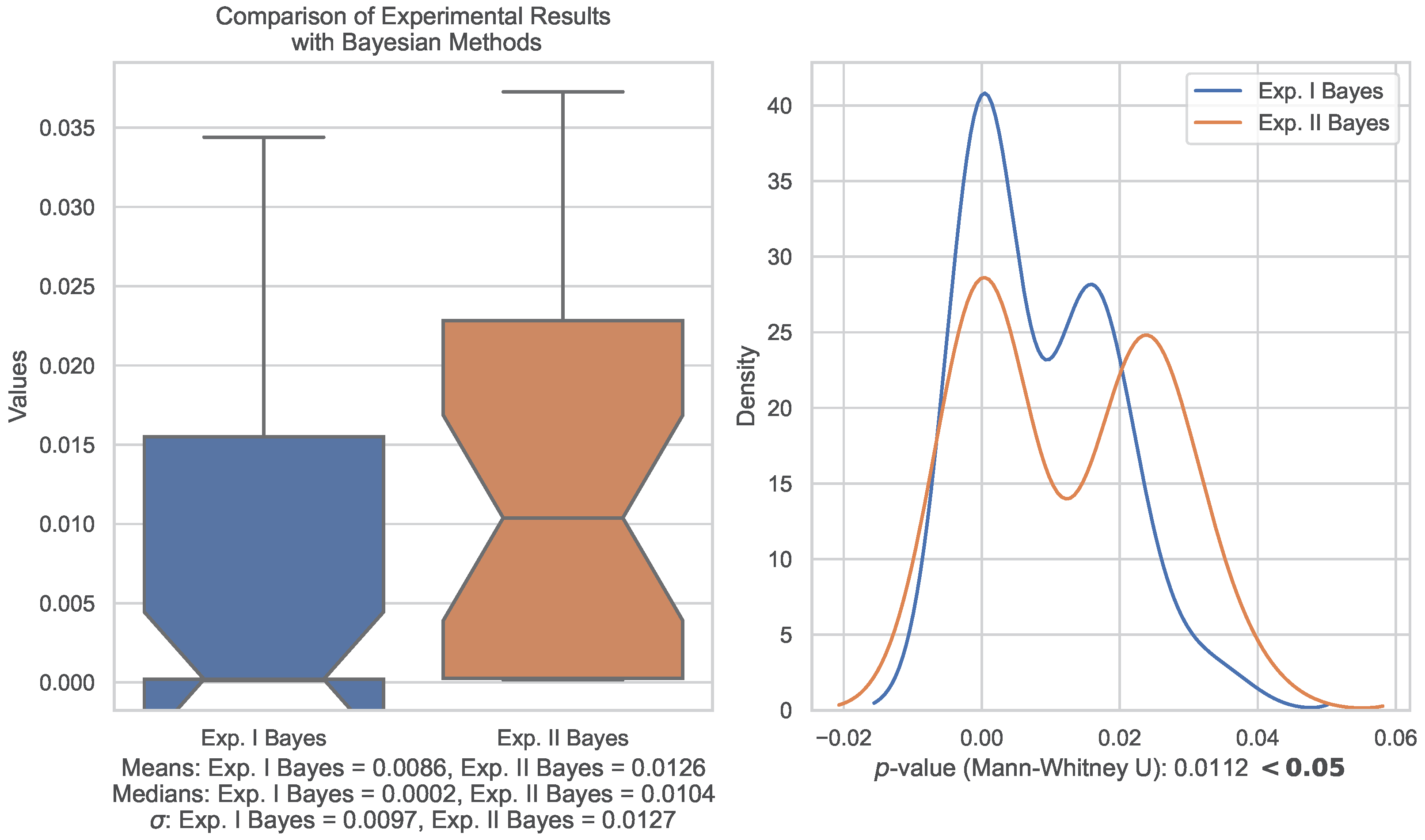
5.3. Comparison of Experiments I and II
A comparative analysis of the CO2e results of Experiments I and II, with respect to the Bayes algorithm, was carried out. The means, medians, standard deviations, and interquartile ranges (IQR) were calculated for both samples. Additionally, the Mann–Whitney U statistical test was performed to determine if there were significant differences between the samples. The p-value is a measure of the probability of obtaining the observed results if there are no real differences between the samples. A p-value less than 0.05 is considered statistically significant, which means that it is unlikely that the observed results are due to chance. The results are presented in Figure 4.

Figure 4.
The figure shows the results of the calculation of the means, medians, standard deviations, and interquartile ranges (IQR) for both samples. It also shows the result of the Mann–Whitney U statistical test, which determined if there are significant differences between the samples.
6. Discussion
The results of the analysis provide valuable insights into the performance and energy efficiency of different classification models and AutoML optimization techniques for a multiclass problem.
A trade-off emerges between predictive performance and energy efficiency in machine-learning models, where the more complex models like Gradient Boosting, Random Forest, and Support Vector Machines achieve remarkable accuracy and F1 scores but also exhibit significantly higher energy consumption and CO2e emissions. In contrast, simpler models like Decision Trees, Naive Bayes, and Linear SVM offer lower emissions but come at the cost of diminished predictive performance. Specifically, the complex models attain 2–5% higher precision in metrics such as accuracy and F1 yet simultaneously demonstrate a 5 to 10-fold surge in energy consumption and emissions. For example, while Random Forest achieves an impressive accuracy of 0.94, it emits 0.014 kg of CO2e, whereas Decision Trees, with an accuracy of 0.92, emit a mere 0.0001 kg of CO2e. In relative terms, Decision Trees offer a 2% reduction in accuracy while achieving a staggering 99% reduction in CO2e emissions compared to Random Forest, illustrating the inherent trade-off between predictive performance and energy efficiency/emissions. Thus, simpler models like Decision Trees and Naive Bayes, though green in their minimal processing requirements, involve some sacrifice in precision, aligning with established research confirming the link between heightened model complexity and elevated computational costs [25].
In Bayesian optimization, the primary hyperparameters under consideration included the number of estimators in Random Forest (ranging from 100 to 500 trees), the maximum tree depth in Decision Trees (varying from 5 to 20 levels), and the number of boosting iterations in Gradient Boosting (ranging from 50 to 200). The selection of these search ranges was guided by recommendations from the existing literature. Conversely, in a random search, these same hyperparameters were randomly sampled.
Bayesian search notably enhanced the balanced accuracy for Gradient Boosting (0.9309 vs. 0.9256) by identifying near-optimal values around 150 boosting iterations. Nonetheless, in a broader context, both approaches yielded similar performance metrics for the primary models. For instance, with Random Forest, Bayesian search achieved an accuracy of 0.9414 using 300 estimators, while random search reached 0.9415 with 250 estimators. A comprehensive exploration of the subtle differences in optimization performance would necessitate further in-depth investigations into hyperparameter responses and the search space.
By meticulously examining specific hyperparameters and search ranges, we gain valuable technical insights into the AutoML optimization process. Although both Bayesian and random search methods demonstrated comparable metrics for the leading models, a more exhaustive analysis of the minor discrepancies could reveal the relative strengths of each method. Both methods achieved favorable outcomes in AutoML optimization, with similar performance metrics under both techniques. Bayesian optimization held a slight advantage in fine-tuning particular models like Gradient Boosting, but the differences were marginal, confirming the feasibility of both methods as AutoML optimizers. This finding aligns with prior research, which consistently highlights the similar performance levels achieved by these hyperparameter tuning methodologies [38].
The results of the analysis show that the CO2e values in the Bayes sample of Experiment II tend to be higher, more dispersed, and wider in terms of interquartile range compared to the Bayes sample of Experiment I. Additionally, the Mann–Whitney U test shows that the Bayes samples of Experiment I and Experiment II have significant differences, as the p-value (0.015523) is less than 0.05, which is the significance level (Figure 4).
The importance of these findings lies in the verification that the proposal outlined in the context of the proof of concept, which consists of the incorporation of metrics related to energy efficiency, leads to the obtainment of machine-learning models characterized by a lower carbon footprint and by their greater agreement with the precepts of Green AI. Despite the inherent limitations of the restricted dataset and the small number of algorithms evaluated, the empirical results allow us to maintain that it is plausible to extrapolate such conclusions to AutoML tools and to other instances of structured data classification that present similarities in terms of the imbalanced class problem.
The discoveries of this study are significant because they provide practical guidance on how to develop and deploy AutoML models more sustainably. The results can be used to inform the design of new AutoML algorithms and to guide the selection of appropriate models for specific problems and energy efficiency metrics.
In summary, it is observed that there is a trade-off between predictive performance and energy efficiency. More complex models have superior predictive performance but also have higher energy consumption and CO2e emissions. A valuable contribution is made to the field of Green AI by demonstrating the feasibility of integrating environmental sustainability into AutoML.
7. Conclusions and Future Research Directions
This study proposed a strategy to improve the energy efficiency of AutoML through hyperparameter optimization using Bayesian and random search algorithms. The experimental results from the proof of concept confirm the viability of developing sustainable AutoML from an energy perspective. This research and its findings are aligned with the Green AI paradigm, whose goal is to reduce the ecological footprint of the entire AutoML process and AI in general.
The results highlight the importance of sustainability in the AutoML context. Energy efficiency was improved through hyperparameter optimization in Bayesian and random search strategies, with the aim of decreasing its environmental impact. These findings indicate that it is feasible to implement concrete measures to reduce the environmental impact of AutoML without negatively affecting other performance metrics, steering it towards greater sustainability and aligning it with the general efforts to make artificial intelligence more environmentally friendly.
The future research proposals are oriented towards the development of prototypes that encompass the evaluation of a broader range of AutoML tools and algorithms, the exploration of various hyperparameter optimization strategies and techniques, the creation of new lightweight and efficient ML architectures, and the ongoing investigation of methods to reduce the carbon footprint throughout the entire ML lifecycle, including data preprocessing, model training, deployment, and inference.
Author Contributions
D.C.-N. and L.G.-F. participated in the conception and design of the work; D.C.-N. and L.G.-F. reviewed the bibliography; D.C.-N. and L.G.-F. conceived and designed the experiments; D.C.-N. and L.G.-F. performed the experiments; D.C.-N. and L.G.-F. analyzed the data; D.C.-N. and L.G.-F. wrote and edited the paper. All authors have read and agreed to the published version of the manuscript.
Funding
This work has been possible thanks to the collaboration and support of the Emerging Heterogeneous Architectures for Machine Learning and Energy Efficiency (TED2021-131019B-I00).
Institutional Review Board Statement
Not applicable.
Informed Consent Statement
Not applicable.
Data Availability Statement
The dataset used is in the public domain. The code can be requested from the authors.
Conflicts of Interest
The authors declare no conflict of interest.
Abbreviations
| AutoML | Automated Machine Learning |
| ML | Machine Learning |
| AI | Artificial Intelligence |
| CPU | Central Processing Unit |
| GPU | Graphics Processing Unit |
| CO2e | Carbon Dioxide Equivalent |
| FLOPs | Floating-point operations per second |
| IQR | Interquartile Ranges |
| KNC | K-Nearest Neighbors Classifier |
| RFC | Random Forest Classifier |
| GBC | Gradient Boosting Classifier |
| DTC | Decision Tree Classifier |
| LSVC | Linear Support Vector Machine |
| SVC | Nonlinear Support Vector Machine |
| GNB | Gaussian Naive Bayes |
References
- Zhou, Z.H. Machine Learning; Springer Nature: Berlin/Heidelberg, Germany, 2021. [Google Scholar]
- Finn, C.; Abbeel, P.; Levine, S. Model-agnostic meta-learning for fast adaptation of deep networks. In Proceedings of the International Conference on Machine Learning, PMLR, Sydney, Australia, 6–11 August 2017; pp. 1126–1135. [Google Scholar]
- Tsiakmaki, M.; Kostopoulos, G.; Kotsiantis, S.; Ragos, O. Implementing AutoML in educational data mining for prediction tasks. Appl. Sci. 2019, 10, 90. [Google Scholar] [CrossRef]
- Preuveneers, D. AutoFL: Towards AutoML in a Federated Learning Context. Appl. Sci. 2023, 13, 8019. [Google Scholar] [CrossRef]
- Shin, J.; Park, K.; Kang, D.K. TA-DARTS: Temperature Annealing of Discrete Operator Distribution for Effective Differential Architecture Search. Appl. Sci. 2023, 13, 10138. [Google Scholar] [CrossRef]
- Zöller, M.A.; Huber, M.F. Benchmark and survey of automated machine learning frameworks. J. Artif. Intell. Res. 2021, 70, 409–472. [Google Scholar] [CrossRef]
- Teixeira, M.C.; Pappa, G.L. Understanding AutoML search spaces with local optima networks. In Proceedings of the Genetic and Evolutionary Computation Conference, Boston, MA, USA, 9–13 July 2022; pp. 449–457. [Google Scholar]
- Tu, R.; Roberts, N.; Prasad, V.; Nayak, S.; Jain, P.; Sala, F.; Ramakrishnan, G.; Talwalkar, A.; Neiswanger, W.; White, C. Automl for climate change: A call to action. arXiv 2022, arXiv:2210.03324. [Google Scholar]
- Hutter, F.; Kotthoff, L.; Vanschoren, J. Automated Machine Learning: Methods, Systems, Challenges; Springer Nature: Berlin/Heidelberg, Germany, 2019. [Google Scholar]
- Yao, Q.; Wang, M.; Chen, Y.; Dai, W.; Li, Y.F.; Tu, W.W.; Yang, Q.; Yu, Y. Taking human out of learning applications: A survey on automated machine learning. arXiv 2018, arXiv:1810.13306. [Google Scholar]
- Schwartz, R.; Dodge, J.; Smith, N.A.; Etzioni, O. Green Ai. Commun. ACM 2020, 63, 54–63. [Google Scholar] [CrossRef]
- Wu, C.J.; Raghavendra, R.; Gupta, U.; Acun, B.; Ardalani, N.; Maeng, K.; Chang, G.; Aga, F.; Huang, J.; Bai, C.; et al. Sustainable ai: Environmental implications, challenges and opportunities. Proc. Mach. Learn. Syst. 2022, 4, 795–813. [Google Scholar]
- Patterson, D.; Gonzalez, J.; Hölzle, U.; Le, Q.; Liang, C.; Munguia, L.M.; Rothchild, D.; So, D.R.; Texier, M.; Dean, J. The carbon footprint of machine learning training will plateau, then shrink. Computer 2022, 55, 18–28. [Google Scholar] [CrossRef]
- Taddeo, M.; Tsamados, A.; Cowls, J.; Floridi, L. Artificial intelligence and the climate emergency: Opportunities, challenges, and recommendations. One Earth 2021, 4, 776–779. [Google Scholar] [CrossRef]
- Dhar, P. The carbon impact of artificial intelligence. Nat. Mach. Intell. 2020, 2, 423–425. [Google Scholar] [CrossRef]
- Dunford, R.; Su, Q.; Tamang, E. The Pareto Principle. Plymouth Stud. Sci. 2014, 7, 140–148. [Google Scholar]
- Tornede, T.; Tornede, A.; Hanselle, J.; Mohr, F.; Wever, M.; Hüllermeier, E. Towards green automated machine learning: Status quo and future directions. J. Artif. Intell. Res. 2023, 77, 427–457. [Google Scholar] [CrossRef]
- Bliek, L. A survey on sustainable surrogate-based optimisation. Sustainability 2022, 14, 3867. [Google Scholar] [CrossRef]
- Mehta, Y.; Xu, R.; Lim, B.; Wu, J.; Gao, J. A Review for Green Energy Machine Learning and AI Services. Energies 2023, 16, 5718. [Google Scholar] [CrossRef]
- Al-Jarrah, O.Y.; Yoo, P.D.; Muhaidat, S.; Karagiannidis, G.K.; Taha, K. Efficient machine learning for big data: A review. Big Data Res. 2015, 2, 87–93. [Google Scholar] [CrossRef]
- Zhong, S.; Zhang, K.; Bagheri, M.; Burken, J.G.; Gu, A.; Li, B.; Ma, X.; Marrone, B.L.; Ren, Z.J.; Schrier, J.; et al. Machine learning: New ideas and tools in environmental science and engineering. Environ. Sci. Technol. 2021, 55, 12741–12754. [Google Scholar] [CrossRef] [PubMed]
- Yarally, T.; Cruz, L.; Feitosa, D.; Sallou, J.; Van Deursen, A. Uncovering Energy-Efficient Practices in Deep Learning Training: Preliminary Steps Towards Green AI. In Proceedings of the 2023 IEEE/ACM 2nd International Conference on AI Engineering–Software Engineering for AI (CAIN), Melbourne, Australia, 15–16 May 2023; IEEE: Piscataway Township, NJ, USA, 2023; pp. 25–36. [Google Scholar]
- Wu, M.; Wang, L.; Xu, J.; Hu, P.; Xu, P. Adaptive surrogate-assisted multi-objective evolutionary algorithm using an efficient infill technique. Swarm Evol. Comput. 2022, 75, 101170. [Google Scholar] [CrossRef]
- Menghani, G. Efficient deep learning: A survey on making deep learning models smaller, faster, and better. ACM Comput. Surv. 2023, 55, 1–37. [Google Scholar] [CrossRef]
- Strubell, E.; Ganesh, A.; McCallum, A. Energy and policy considerations for deep learning in NLP. arXiv 2019, arXiv:1906.02243. [Google Scholar]
- Lacoste, A.; Luccioni, A.; Schmidt, V.; Dandres, T. Quantifying the carbon emissions of machine learning. arXiv 2019, arXiv:1910.09700. [Google Scholar]
- Tan, M.; Le, Q. Efficientnet: Rethinking model scaling for convolutional neural networks. In Proceedings of the International Conference on Machine Learning, PMLR, Long Beach, CA, USA, 9–15 June 2019; pp. 6105–6114. [Google Scholar]
- Feurer, M.; Hutter, F. Hyperparameter optimization. In Automated Machine Learning: Methods, Systems, Challenges; Springer: Cham, Switzerland; Berlin, Germany, 2019; pp. 3–33. [Google Scholar]
- Mirzadeh, S.I.; Farajtabar, M.; Li, A.; Levine, N.; Matsukawa, A.; Ghasemzadeh, H. Improved knowledge distillation via teacher assistant. In Proceedings of the AAAI Conference on Artificial Intelligence, New York, NY, USA, 7–12 February 2020; Volume 34, pp. 5191–5198. [Google Scholar]
- Vázquez-Canteli, J.R.; Nagy, Z. Reinforcement learning for demand response: A review of algorithms and modeling techniques. Appl. Energy 2019, 235, 1072–1089. [Google Scholar] [CrossRef]
- Anthony, L.F.W.; Kanding, B.; Selvan, R. Carbontracker: Tracking and predicting the carbon footprint of training deep learning models. arXiv 2020, arXiv:2007.03051. [Google Scholar]
- Han, S.; Mao, H.; Dally, W.J. Deep compression: Compressing deep neural networks with pruning, trained quantization and huffman coding. arXiv 2015, arXiv:1510.00149. [Google Scholar]
- Henderson, P.; Hu, J.; Romoff, J.; Brunskill, E.; Jurafsky, D.; Pineau, J. Towards the systematic reporting of the energy and carbon footprints of machine learning. J. Mach. Learn. Res. 2020, 21, 10039–10081. [Google Scholar]
- Hooker, S.; Dauphin, Y.; Courville, A.; Frome, A. Selective Brain Damage: Measuring the Disparate Impact of Model Pruning. In Proceedings of the International Conference on Learning Representations (ICLR), Addis Ababa, Ethiopia, 26 April–1 May 2019. [Google Scholar]
- Bergstra, J.; Yamins, D.; Cox, D.D. Hyperopt: A python library for optimizing the hyperparameters of machine learning algorithms. In Proceedings of the 12th Python in Science Conference, Citeseer, Austin, TX, USA, 24 June–29 June 2013; Volume 13, p. 20. [Google Scholar]
- Probst, P.; Boulesteix, A.L.; Bischl, B. Tunability: Importance of hyperparameters of machine learning algorithms. J. Mach. Learn. Res. 2019, 20, 1934–1965. [Google Scholar]
- Claesen, M.; De Moor, B. Hyperparameter search in machine learning. arXiv 2015, arXiv:1502.02127. [Google Scholar]
- Yang, L.; Shami, A. On hyperparameter optimization of machine learning algorithms: Theory and practice. Neurocomputing 2020, 415, 295–316. [Google Scholar] [CrossRef]
- Verdecchia, R.; Sallou, J.; Cruz, L. A systematic review of Green AI. In Wiley Interdisciplinary Reviews: Data Mining and Knowledge Discovery; Wiley: Hoboken, NJ, USA, 2023; p. e1507. [Google Scholar]
- Candelieri, A.; Perego, R.; Archetti, F. Green machine learning via augmented Gaussian processes and multi-information source optimization. Soft Computing 2021, 25, 12591–12603. [Google Scholar] [CrossRef]
- Bachoc, F. Cross validation and maximum likelihood estimations of hyper-parameters of Gaussian processes with model misspecification. Comput. Stat. Data Anal. 2013, 66, 55–69. [Google Scholar] [CrossRef]
- Snoek, J.; Larochelle, H.; Adams, R.P. Practical bayesian optimization of machine learning algorithms. Adv. Neural Inf. Process. Syst. 2012, 2, 2951–2959. [Google Scholar]
- Sun, X.; Lin, J.; Bischl, B. Reinbo: Machine learning pipeline search and configuration with bayesian optimization embedded reinforcement learning. arXiv 2019, arXiv:1904.05381. [Google Scholar]
- Shahriari, B.; Swersky, K.; Wang, Z.; Adams, R.P.; De Freitas, N. Taking the human out of the loop: A review of Bayesian optimization. Proc. IEEE 2015, 104, 148–175. [Google Scholar] [CrossRef]
- Stamoulis, D.; Cai, E.; Juan, D.C.; Marculescu, D. Hyperpower: Power-and memory-constrained hyper-parameter optimization for neural networks. In Proceedings of the 2018 Design, Automation & Test in Europe Conference & Exhibition (DATE), Dresden, Germany, 19–23 March 2018; IEEE: Piscataway Township, NJ, USA, 2018; pp. 19–24. [Google Scholar]
- de Chavannes, L.H.P.; Kongsbak, M.G.K.; Rantzau, T.; Derczynski, L. Hyperparameter power impact in transformer language model training. In Proceedings of the Second Workshop on Simple and Efficient Natural Language Processing, Online, 10 November 2021; pp. 96–118. [Google Scholar]
- Polino, A.; Pascanu, R.; Alistarh, D. Model compression via distillation and quantization. arXiv 2018, arXiv:1802.05668. [Google Scholar]
- Sze, V.; Chen, Y.H.; Yang, T.J.; Emer, J.S. Efficient processing of deep neural networks: A tutorial and survey. Proc. IEEE 2017, 105, 2295–2329. [Google Scholar] [CrossRef]
- Romero, A.; Ballas, N.; Kahou, S.E.; Chassang, A.; Gatta, C.; Bengio, Y. Fitnets: Hints for thin deep nets. arXiv 2014, arXiv:1412.6550. [Google Scholar]
- Asperti, A.; Evangelista, D.; Loli Piccolomini, E. A survey on variational autoencoders from a green AI perspective. SN Comput. Sci. 2021, 2, 301. [Google Scholar] [CrossRef]
- Sønderby, C.K.; Raiko, T.; Maaløe, L.; Sønderby, S.K.; Winther, O. Ladder variational autoencoders. Adv. Neural Inf. Process. Syst. 2016, 29, 3745–3753. [Google Scholar]
- Glorot, X.; Bengio, Y. Understanding the difficulty of training deep feedforward neural networks. In Proceedings of the Thirteenth International Conference on Artificial Intelligence and Statistics, JMLR Workshop and Conference Proceedings, Sardinia, Italy, 13–15 May 2010; pp. 249–256. [Google Scholar]
- Bergstra, J.; Bengio, Y. Random search for hyper-parameter optimization. J. Mach. Learn. Res. 2012, 13, 281–305. [Google Scholar]
- Ulyanov, D.; Vedaldi, A.; Lempitsky, V. Deep image prior. In Proceedings of the IEEE Conference on Computer Vision and Pattern Recognition, Salt Lake City, UT, USA, 18–23 June 2018; pp. 9446–9454. [Google Scholar]
- Morales-Hernández, A.; Van Nieuwenhuyse, I.; Rojas Gonzalez, S. A survey on multi-objective hyperparameter optimization algorithms for machine learning. Artif. Intell. Rev. 2023, 56, 8043–8093. [Google Scholar] [CrossRef]
- Kim, Y.H.; Reddy, B.; Yun, S.; Seo, C. Nemo: Neuro-evolution with multiobjective optimization of deep neural network for speed and accuracy. In Proceedings of the ICML 2017 AutoML Workshop, Sydney, Australia, 10 August 2017; pp. 1–8. [Google Scholar]
- Wilson, A.G.; Dann, C.; Lucas, C.; Xing, E.P. The human kernel. Adv. Neural Inf. Process. Syst. 2015, 2, 2854–2862. [Google Scholar]
- Zoph, B.; Vasudevan, V.; Shlens, J.; Le, Q.V. Learning transferable architectures for scalable image recognition. In Proceedings of the IEEE Conference on Computer Vision and Pattern Recognition, Salt Lake City, UT, USA, 18–23 June 2018; pp. 8697–8710. [Google Scholar]
- Han, S.; Pool, J.; Tran, J.; Dally, W. Learning both weights and connections for efficient neural network. Adv. Neural Inf. Process. Syst. 2015, 1, 1135–1143. [Google Scholar]
- Hinton, G.; Vinyals, O.; Dean, J. Distilling the knowledge in a neural network. arXiv 2015, arXiv:1503.02531. [Google Scholar]
- Yang, J.; Martinez, B.; Bulat, A.; Tzimiropoulos, G. Knowledge distillation via adaptive instance normalization. arXiv 2020, arXiv:2003.04289. [Google Scholar]
- Wolberg, W.; Street, W.; Mangasarian, O. Breast Cancer Wisconsin (Diagnostic) UCI Machine Learning Repository; University of California: Irvine, CA, USA, 1995. [Google Scholar] [CrossRef]
- Oyedeji, S.; Seffah, A.; Penzenstadler, B. A catalogue supporting software sustainability design. Sustainability 2018, 10, 2296. [Google Scholar] [CrossRef]
- Calero, C.; Moraga, M.Á.; Piattini, M. Introduction to Software Sustainability. In Software Sustainability; Calero, C., Moraga, M.Á., Piattini, M., Eds.; Springer International Publishing: Cham, Switzerland, 2021; pp. 1–15. [Google Scholar] [CrossRef]
- Noman, H.; Mahoto, N.A.; Bhatti, S.; Abosaq, H.A.; Al Reshan, M.S.; Shaikh, A. An Exploratory Study of Software Sustainability at Early Stages of Software Development. Sustainability 2022, 14, 8596. [Google Scholar] [CrossRef]
- Calero, C.; Bertoa, M.F.; Moraga, M.Á. A systematic literature review for software sustainability measures. In Proceedings of the 2013 2nd International Workshop on Green and Sustainable Software (GREENS), San Francisco, CA, USA, 20 May 2013; IEEE: Piscataway Township, NJ, USA, 2013; pp. 46–53. [Google Scholar]
- Heguerte, L.B.; Bugeau, A.; Lannelongue, L. How to estimate carbon footprint when training deep learning models? A guide and review. arXiv 2023, arXiv:2306.08323. [Google Scholar] [CrossRef]
- Lannelongue, L.; Grealey, J.; Inouye, M. Green algorithms: Quantifying the carbon footprint of computation. Adv. Sci. 2021, 8, 2100707. [Google Scholar] [CrossRef] [PubMed]
- Patel, Y.S.; Mehrotra, N.; Soner, S. Green cloud computing: A review on Green IT areas for cloud computing environment. In Proceedings of the 2015 International Conference on Futuristic Trends on Computational Analysis and Knowledge Management (ABLAZE), Greater Noida, India, 25–27 February 2015; IEEE: Piscataway Township, NJ, USA, 2015; pp. 327–332. [Google Scholar]
- Maevsky, D.; Maevskaya, E.; Stetsuyk, E. Evaluating the RAM energy consumption at the stage of software development. In Green IT Engineering: Concepts, Models, Complex Systems Architectures; Springer: Berlin/Heidelberg, Germany, 2017; pp. 101–121. [Google Scholar]
- Budennyy, S.; Lazarev, V.; Zakharenko, N.; Korovin, A.; Plosskaya, O.; Dimitrov, D.; Arkhipkin, V.; Oseledets, I.; Barsola, I.; Egorov, I.; et al. Eco2AI: Carbon emissions tracking of machine learning models as the first step towards sustainable AI. arXiv 2022, arXiv:cs.LG/2208.00406. [Google Scholar] [CrossRef]
- Tariq, H.I.; Sohail, A.; Aslam, U.; Batcha, N.K. Loan default prediction model using sample, explore, modify, model, and assess (SEMMA). J. Comput. Theor. Nanosci. 2019, 16, 3489–3503. [Google Scholar] [CrossRef]
Disclaimer/Publisher’s Note: The statements, opinions and data contained in all publications are solely those of the individual author(s) and contributor(s) and not of MDPI and/or the editor(s). MDPI and/or the editor(s) disclaim responsibility for any injury to people or property resulting from any ideas, methods, instructions or products referred to in the content. |
© 2023 by the authors. Licensee MDPI, Basel, Switzerland. This article is an open access article distributed under the terms and conditions of the Creative Commons Attribution (CC BY) license (https://creativecommons.org/licenses/by/4.0/).