SANA: Sensitivity-Aware Neural Architecture Adaptation for Uniform Quantization

Abstract

Uniform quantization is widely taken as an efficient compression method in practical applications. Despite its merit of having a low computational overhead, uniform quantization fails to preserve sensitive components in neural networks when applied with ultra-low bit precision, which could lead to a non-trivial accuracy degradation. Previous works have applied mixed-precision quantization to address this problem. However, finding the correct bit settings for different layers always demands significant time and resource consumption. Moreover, mixed-precision quantization is not well supported on current general-purpose machines such as GPUs and CPUs and, thus, will cause intolerable overheads in deployment. To leverage the efficiency of uniform quantization while maintaining accuracy, in this paper, we propose sensitivity-aware network adaptation (SANA), which automatically modifies the model architecture based on sensitivity analysis to make it more compatible with uniform quantization. Furthermore, we formulated four different channel initialization strategies to accelerate the quantization-aware fine-tuning process of SANA. Our experimental results showed that SANA can outperform standard uniform quantization and other state-of-the-art quantization methods in terms of accuracy, with comparable or even smaller memory consumption. Notably, ResNet-50-SANA (24.4 MB) with W4A8 quantization achieved 77.8% top-one accuracy on ImageNet, which even surpassed the 77.6% of the full-precision ResNet-50 (97.8 MB) baseline.

1. Introduction

Large neural network models generally require high computational and memory resources and are challenging to deploy in resource-constrained environments. Quantization [1,2,3] has shown great success to address this problem and achieve efficient deep learning. By reducing the precision of model parameters, quantization reduces storage and computational cost and enables the deployment of large over-parameterized models on mobile platforms such as phones or smart speakers.

Uniform quantization is a mainstream quantization method due to its simplicity and efficiency, but it could lead to performance degradation when applied with an ultra-low bitwidth (4 bit or less). For example, directly performing W3A8 on ResNet-50 will lead to significant accuracy degradation (from 77% to 70%) [4], even with dedicated re-training. In order to preserve important components in the pre-trained model, mixed-precision quantization [3,5] has been proposed in previous works to narrow the accuracy gap by assigning higher precision to more-sensitive layers. However, the improvement comes at the cost of a substantial demand for computational resources and non-negligible time and space consumption in hardware deployment. It should be noted that the implementation overhead is even more severe in the case of general-purpose machines (GPUs and CPUs).

In this paper, we aimed to maintain the simplicity and meanwhile improve the accuracy with sensitivity-aware model architecture adaptation. We found that some models may be more sensitive to the disturbance of quantization due to their complicated architectures and heavily fine-tuned parameters. We analyzed the sensitivity of models and automatically adjusted the model architecture accordingly to make it more compatible with uniform quantization. Specifically, the model architecture can be adapted by increasing the size of the channels in the convolution layers while making necessary accommodations to the regularization layers. The adapted architecture can then be fine-tuned to achieve better performance. To speed up this process, we formulated four initialization strategies, Halving, Zero Padding, Averaging, and Small Int. The effectiveness of different initialization strategies was evaluated based on the experimental results in Section 4. In summary, the contribution of this paper includes three aspects:

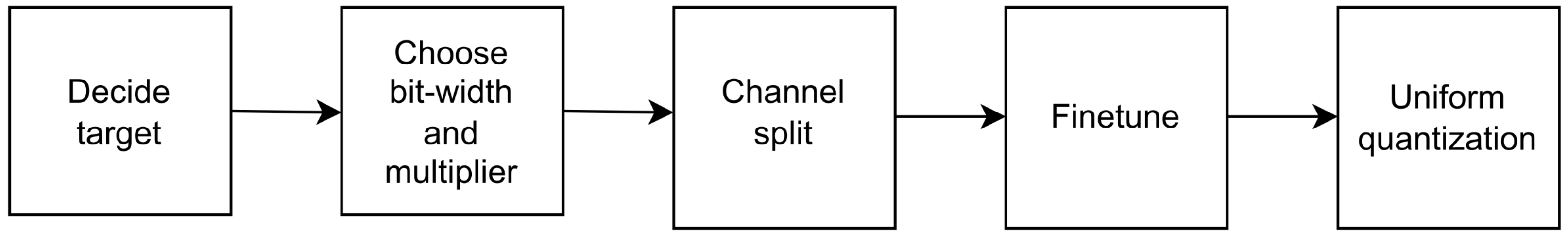
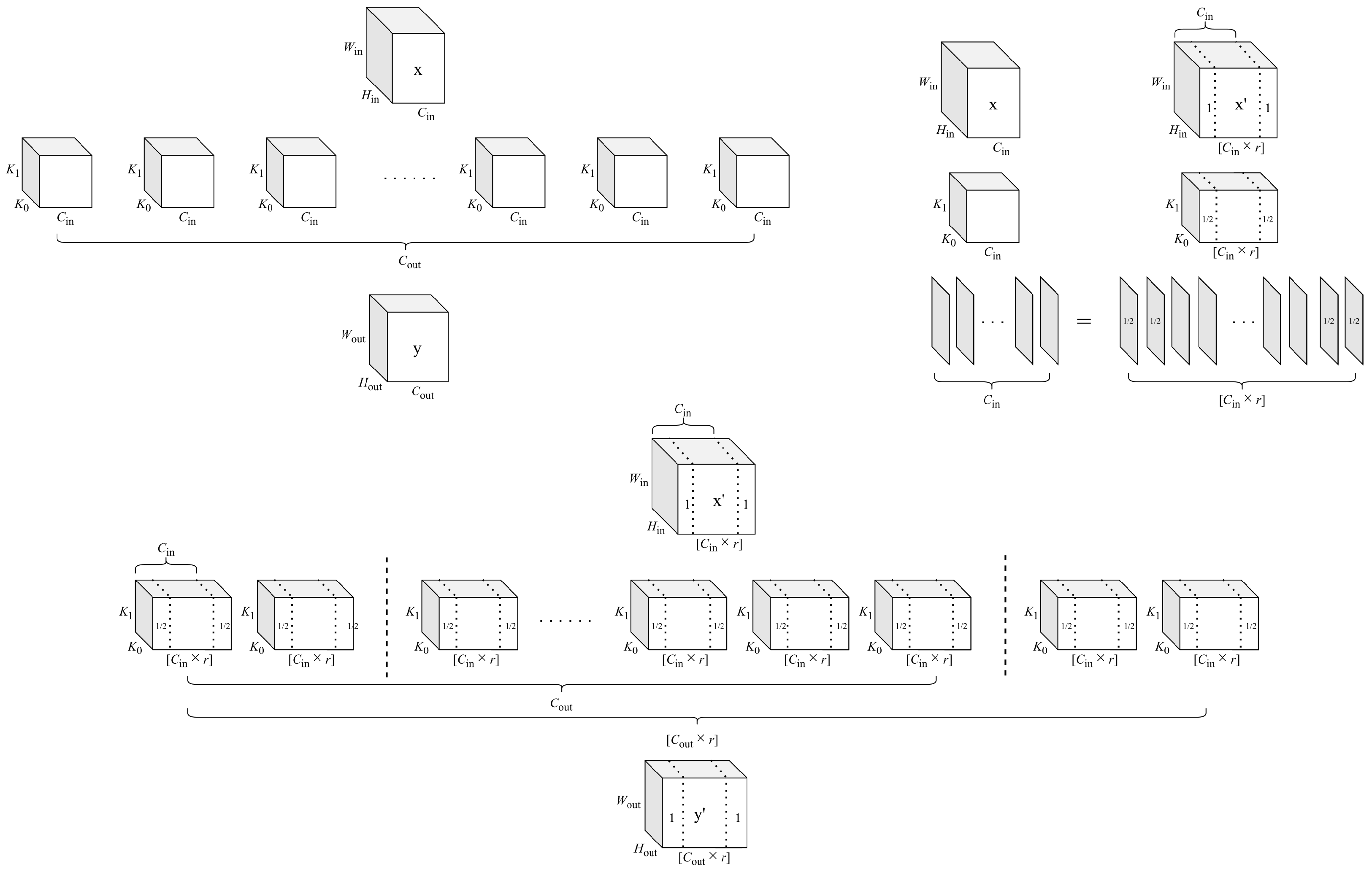
• We propose sensitivity-aware neural architecture adaptation to automatically make the original model friendly to uniform quantization. Our model is cost-friendly compared to neural architecture search (NAS) and outperformed direct uniform quantization or mixed-precision quantization.
• We formulated four initialization strategies to quicken the quantization-aware fine-tuning process.
• Our approach provides a practical and simple solution, with the W4A8 ResNet-50-SANA model achieving 77.8% accuracy, which surpassed the 77.6% accuracy of the full-precision ResNet-50 model.

2. Related Work

2.1. Post-Training Quantization

Post-training quantization (PTQ) directly computes the quantization parameters without any training or fine-tuning. Unlike quantization-aware training (QAT), labeled data or high computational power are not required for PTQ. However, this benefit often comes at the expense of non-trivial accuracy degradation, especially when using low-precision quantization [6,7,8]. Several methods have been proposed to address the challenges of PTQ [9,10]. Choukroun et al. [11] proposed the optimal MSE method to minimize the $L_2$ distance between the quantized model and the pretrained model. Banner et al. [12] developed a channelwise quantization approach that computes clipping thresholds and bits allocated for each channel. To solve the outlier channel problem, Zhao et al. [13] introduced an outlier-channel-splitting (OCS) method to split the channels with extreme values. Another notable work is AdaRound, proposed by Nagel et al. [14], showing that a weight-rounding mechanism that adapts to the data and the task loss outperformed the naive round-to-nearest method. Liu et al. [15] proposed an adaptive floating point (AFP) with a flexible configuration of the exponent and mantissa segments. In situations where training data may be inaccessible, Cai et al. [16] matched the statistics of batch normalization to synthesize the calibration data. Liu et al. [17] proposed a zero-shot adversarial quantization (ZAQ) framework utilizing generative adversarial networks (GANs) to generate realistic data when the available data are insufficient for calibration.

2.2. Mixed-Precision Quantization

Conventional quantization approaches project full-precision weights and activations to fixed-point numbers, using the same bitwidth for all layers of a network [18]. However, mixed-precision quantization provides flexibility in selecting different precisions for different network layers [19,20,21]. Selecting mixed-precision for each layer can be seen as a searching problem, and many methods have been proposed to solve it [2,3,22,23]. In particular, Wang et al. [3] leveraged reinforcement learning (RL) to automatically determine the quantization policy and took the hardware accelerator as part of the RL agent feedback. Wu et al. [24] converted the bitwidth search into a neural architecture search (NAS) problem and explored the search space using the differentiable NAS (DNAS) method [25]. Different from these exploration-based approaches, Dong et al. [5,26] introduced HAWQ, which measures the layer sensitivity based on the trace of the second-order operator, which is faster than exploration-based mixed-precision methods.

2.3. Neural Architecture Search

Automated machine learning (AutoML) has been gaining increased attention in recent years, with a strong emphasis on the automation of parameter selection and the fine-tuning of the model architecture [27]. A notable idea in this domain is model architecture adaptation, which reduces the need to design neural networks from scratch. Neural architecture search (NAS) [28,29,30], in particular, aims to find the optimal architecture for a specific problem by using methods such as reinforcement learning and evolutionary algorithms [25,31,32]. Both AutoML and NAS have been employed to adapt neural architectures with notable results [33,34].

Furthermore, model adaptation has also been integrated with other optimization avenues, such as quantization. Previous research has focused on joint optimization for the neural architecture and quantization space, which has been shown to be effective in achieving significant performance gains and has inspired broad interest. Specifically, Gong et al. [35] explored the end-to-end co-optimization of NAS and mixed-precision quantization. Furthermore, Wang et al. [36] used a predictor–transfer technique to obtain a quantization-aware predictor, which was then fed into the evolutionary search to jointly optimize the neural network architecture, pruning policy, and quantization policy.

3. Methodology

3.1. Motivation

Uniform quantization is efficient and simple to deploy on general computation hardware compared with mixed-precision quantization. However, mixed-precision quantization can bridge the accuracy gap more effectively under the same memory constraint by assigning bits and discretizing distributions in a non-uniform manner. One of the key differences between these techniques is that uniform quantization overlooks the importance of keeping sensitive and efficient layers of higher precision to save time and resources. In contrast, mixed-precision quantization allocates more bits to more-sensitive layers and fewer bits to less-sensitive layers, resulting in higher performance.

To close the accuracy gap, we can either assign higher bitwidths to sensitive layers, as done in mixed-precision quantization, or enhance their robustness to uniform quantization. Taking inspiration from [37], we attempted to reduce the model’s sensitivity by splitting its channels. Our hypothesis is that networks with more channels are less sensitive to quantization. There are four reasons supporting our hypothesis. The first is network redundancy. More channels can imply greater redundancy. When quantization is applied, even if some information is lost in a few channels, others can still retain the necessary information for the network to perform well. The second reason is the number of parameters. Networks with more channels usually have more parameters. Even if quantization results in information loss, the overall capability of the model remains. The third reason is feature capture. More channels in the network can capture more features, complex patterns, and higher-order statistics, which might be less affected by quantization. The forth is the model width. Intuitively, wider layers can capture finer-grained patterns on larger images, making them less sensitive to quantization.

Our work performed uniform quantization on the adopted models with extra channels, which is simple and straightforward to deploy on general devices and saves computational resources. We accommodated a neural network for uniform quantization using channel splitting and then applied uniform quantization with lower bits on the expanded larger network to fit within the desired memory constraint. Our approach works automatically on the selected models, optimizing the trade-off between quantization and model sensitivity. The whole process is illustrated in Figure 1.

Consider a layer that takes a vector $\mathbf{x}={\left\{{\mathbf{x}}_i\right\}}_{i=0}^{C_{\mathrm{in}}}$ as the input and a vector $\mathbf{y}={\left\{{\mathbf{y}}_j\right\}}_{j=0}^{C_{\mathrm{out}}}$ as the output.

$${\mathbf{y}}_j=\sum _{i=1}^{C_{\mathrm{in}}}{\mathbf{x}}_i\ast {\mathbf{W}}_{i,j}$$

(1)

In this equation, ${\mathbf{W}}_{i,j}$ denotes the weights and ∗ operator stands for either matrix multiplication or 2D convolution. To resize the layer, we introduce a multiplier r ($r\in (1,2]$):

$${\mathbf{y}}_j^{\prime }=\sum _{i=1}^{[C_{\mathrm{in}}\times r]}{\mathbf{x}}_i^{\prime }\ast {\mathbf{W}}_{ij}^{\prime }$$

(2)

Here, ${\mathbf{x}}^{\prime }={\left\{{\mathbf{x}}_i^{\prime }\right\}}_{i=0}^{[C_{\mathrm{in}}\times r]}$ and ${\mathbf{y}}^{\prime }={\left\{{\mathbf{y}}_j^{\prime }\right\}}_{j=0}^{[C_{\mathrm{out}}\times r]}$ are the resized input vector and the resized output vector, respectively. $\left[\right]$ represents a rounding operation that rounds the number to the nearest integer and truncates the fractional part. To meet the memory constraint, we expanded the entire network using this formula and then uniformly quantized it into a lower bitwidth than the target, rather than quantizing the original network to the target bitwidth. We can approximately estimate the model size and determine the appropriate multiplier r. The number of parameters in $\mathbf{W}$ would be $C_{\mathrm{in}}\times C_{\mathrm{out}}$, and the number of parameters in ${\mathbf{W}}^{\prime }$ would be $[C_{\mathrm{in}}\times r]\times [C_{\mathrm{out}}\times r]$.

$$C_{\mathrm{in}}\times C_{\mathrm{out}}\times b_t=[C_{\mathrm{in}}\times r]\times [C_{\mathrm{out}}\times r]\times b$$

(3)

Based on the number of parameters in the weight matrices, we can choose the appropriate multiplier r. In Formula (3), $b_t$ represents the target bitwidth for the base model and b represents the scaled bitwidth for the expanded model. Usually, $b_t$ is determined by the target memory usage and b is determined by the network itself, which will be further discussed later. With $b_t$ and b, we can determine the multiplier r:

$$r=\sqrt{\frac{b_t}{b}}$$

(4)

For instance, if we set the target bitwidth at 8 bit and the scaled bitwidth at 4 bit, then the multiplier r is $\sqrt{\frac{8}{4}}=\sqrt{2}$.

In this paragraph, we will explain how b is determined by the network. Though networks with more channels are generally less sensitive to quantization, the benefit of channel splitting is different for different networks. To further examine the hypothesis, we also investigated the relationship between the network size and sensitivity to quantization by conducting empirical experiments on redundant models and compact models respectively. The results are shown in Section 4.

To save training time, we also formulated four extra channel-allocation strategies, which will be discussed in the following section. These strategies allow the expanded model to inherit a significant portion of the pre-trained weights from the base model, eliminating the need to train from scratch and quickening the fine-tuning process.

3.2. Uniform Quantization

The uniform quantization function is defined as follows:

$$Q\left(r\right)=\left[\frac{r}{S}\right]-Z$$

(5)

In this equation, Q represents the quantization function, r represents the input (activation or weight), S represents the real-valued scaling factor, and Z represents the integer zero point. The choice of the integer zero point in quantization can determine whether the quantization is symmetric or asymmetric. Since symmetric quantization is one of the most-straightforward quantization strategies, we implemented symmetric quantization to contribute to making our approach simpler. In full-range symmetric quantization, the integer zero point Z is set to 0 to reduce the computational cost during inference, and the real-valued scaling factor S is given by:

$$S=\frac{max\left(\right|r\left|\right)}{2^{b-1}-1}$$

(6)

where b is the quantization bitwidth.

In asymmetric quantization, the real-valued scaling factor S is defined as:

$$S=\frac{\beta -\alpha }{2^b-1}$$

(7)

where $\alpha$ and $\beta$ denote the minimum and maximum values for the clipping range (i.e., $\alpha =r_{\min }$ and $\beta =r_{\max }$).

3.3. Initialization

A good initialization is helpful for the training process to achieve better performance, while a poor initialization can result in slow convergence and high variance, requiring extra time for training to reach satisfactory performance. To alleviate the problem and speed up the quantization-aware fine-tuning process, we explored four different ways to initialize the neural network parameters effectively: (1) Halving, (2) Zero Padding, (3) Averaging, and (4) Small Int. The network remains functionally identical when using either Halving or Zero Padding, which explains why it requires less training time. We explain each method in detail as follows.

Halving: Inspired by outlier channel splitting (OCS) [38], we divided the values in the first $[C_{\mathrm{in}}\times r]-C_{\mathrm{in}}$ channels by 2 and allocated the extra channels with the same divided values. This approach creates a functionally identical network and reduces the range of the distribution. We can define a convolution layer as in Equation (1). The input size is $\left(N,C_{\mathrm{in}},H_{\mathrm{in}},W_{\mathrm{in}}\right)$, and the output size is $(N,C_{\mathrm{out}},H_{\mathrm{out}},W_{\mathrm{out}})$.

Here, N represents the batch size, C denotes the number of channels, H and W represent the height and width in pixels, ${\mathbf{W}}_{i,j}$ represents the weights, and ∗ represents either matrix multiplication or 2D convolution. For convolution, the size of the weights is $(C_{\mathrm{out}},C_{\mathrm{in}},K_0,K_1)$, and $(K_0,K_1)$ is the size of the convolving kernel. We analyzed one batch at a time. In the following discussion, the size of $\mathbf{x}$ is $(C_{\mathrm{in}},H_{\mathrm{in}},W_{\mathrm{in}})$ and the size of $\mathbf{y}$ is $(C_{\mathrm{out}},H_{\mathrm{out}},W_{\mathrm{out}})$.

After channel splitting, the size of ${\mathbf{W}}^{\prime }$ is $([C_{\mathrm{out}}\times r],[C_{\mathrm{in}}\times r],K_0,K_1)$. To match the size of the weights, we split the input $\mathbf{x}={\left\{{\mathbf{x}}_i\right\}}_{i=0}^{C_{\mathrm{in}}}$ with the formula below:

$${\mathbf{x}}_i^{\prime }=\left\{\begin{array}{cc}{\mathbf{x}}_i\hfill & 1\le i\le C_{\mathrm{in}}\hfill \\ {\mathbf{x}}_{i-C_{\mathrm{in}}}\hfill & C_{\mathrm{in}}+1\le i\le [C_{\mathrm{in}}\times r]\hfill \end{array}\right.$$

(8)

To ensure the correctness of forward propagation, the output ${\mathbf{y}}_j^{\prime }$ must also follow the same splitting rule:

$${\mathbf{y}}_j^{\prime }=\left\{\begin{array}{cc}{\mathbf{y}}_j\hfill & 1\le j\le C_{\mathrm{out}}\hfill \\ {\mathbf{y}}_{j-C_{\mathrm{out}}}\hfill & C_{\mathrm{out}}+1\le j\le [C_{\mathrm{out}}\times r]\hfill \end{array}\right.$$

(9)

Without loss of generality, we halved the values in the first $s_{in}$ channels ($s_{in}=[C_{\mathrm{in}}\times r]-C_{\mathrm{in}}$) and rewrote the convolution equation:

$$\begin{array}{cc}\hfill {\mathbf{y}}_j& =\sum _{i=1}^{s_{in}}{\mathbf{x}}_i\ast {\mathbf{W}}_{i,j}+\sum _{i=s_{in}+1}^{C_{\mathrm{in}}}{\mathbf{x}}_i\ast {\mathbf{W}}_{i,j}\hfill \\ \hfill & =\sum _{i=1}^{s_{in}}({\mathbf{x}}_i\ast \frac{{\mathbf{W}}_{i,j}}{2}\times 2)+\sum _{i=s_{in}+1}^{C_{\mathrm{in}}}{\mathbf{x}}_i\ast {\mathbf{W}}_{i,j}\hfill \\ \hfill & =\sum _{i=1}^{s_{in}}{\mathbf{x}}_i\ast \frac{{\mathbf{W}}_{i,j}}{2}+\sum _{i=s_{in}+1}^{C_{\mathrm{in}}}{\mathbf{x}}_i\ast {\mathbf{W}}_{i,j}\hfill \\ \hfill & +\sum _{i=C_{\mathrm{in}}+1}^{[C_{\mathrm{in}}\times r]}{\mathbf{x}}_{i-C_{\mathrm{in}}}\ast \frac{{\mathbf{W}}_{i-C_{\mathrm{in}},j}}{2}\hfill \\ \hfill & =\sum _{i=1}^{[C_{\mathrm{in}}\times r]}{\mathbf{x}}_i^{\prime }\ast {\mathbf{W}}_{i,j}^{″}\hfill \end{array}$$

(10)

We split each of the first $s_{in}$ input channels into two channels, resulting in ${\mathbf{W}}^{″}$ with a size of $(C_{\mathrm{out}},[C_{\mathrm{in}}\times r],K_0,K_1)$. By Halving the weights of these channels, we preserved the equivalence of ${\mathbf{y}}_j$ and ${\mathbf{y}}_j^{\prime }$ when $1\le j\le C_{\mathrm{out}}$. For ${\mathbf{y}}_j^{\prime }$, where $C_{\mathrm{out}}+1\le j\le [C_{\mathrm{out}}\times r]$, we simply duplicated the first $s_{out}$ output channels ($s_{out}=[C_{\mathrm{out}}\times r]-C_{\mathrm{out}}$) of ${\mathbf{W}}^{″}$. Thus, the extra weights are equal to the corresponding weights of the first $s_{out}$ output channels.

$$\begin{array}{cc}\hfill {\mathbf{y}}_j^{\prime }& ={\mathbf{y}}_{j-C_{\mathrm{out}}}=\sum _{i=1}^{[C_{\mathrm{in}}\times r]}{\mathbf{x}}_i^{\prime }\ast {\mathbf{W}}_{i,j-C_{\mathrm{out}}}^{″}\hfill \\ \hfill & =\sum _{i=1}^{[C_{\mathrm{in}}\times r]}{\mathbf{x}}_i^{\prime }\ast {\mathbf{W}}_{i,j}^{\prime }\hfill \end{array}$$

(11)

We expanded certain channels in the weights and scaled the layer with factor r while preserving functional equivalence. To achieve this, we halved and duplicated the values in the first $s_{in}$ channels ($s_{in}=[C_{\mathrm{in}}\times r]-C_{\mathrm{in}}$) to obtain ${\mathbf{W}}^{″}$. After duplication, we obtain ${\mathbf{W}}_{i,j-C_{\mathrm{out}}}^{″}={\mathbf{W}}_{i,j}^{\prime }$ for $C_{\mathrm{out}}+1\le j\le [C_{\mathrm{out}}\times r]$. The size of ${\mathbf{W}}^{\prime }$ is $([C_{\mathrm{out}}\times r],[C_{\mathrm{in}}\times r],K_0,K_1)$. In Figure 2, we illustrate the process of neural architecture adaption with Halving initialization.

Zero Padding: In digital signal processing, Zero Padding is typically employed to make the length of a signal a power of two by extending the signal with zeros. Inspired by this, we initialized the weights of the extra channels to zeros to keep the generality of the model. After splitting inputs $\mathbf{x}$ and $\mathbf{y}$ as Equations (8) and (9), we can rewrite the convolution equation as in Equation (10). Note that ${\mathbf{0}}_{C_{\mathrm{out}}\times ([C_{\mathrm{in}}\times r]-C_{\mathrm{in}})\times K_0\times K_1}$ is an all-zero matrix with a size of $(C_{\mathrm{out}},[C_{\mathrm{in}}\times r],K_0,K_1)$.

$$\begin{array}{cc}\hfill {\mathbf{y}}_j& =\sum _{i=1}^{C_{in}}{\mathbf{x}}_i\ast {\mathbf{W}}_{i,j}+\sum _{i=C_{\mathrm{in}}+1}^{[C_{\mathrm{in}}\times r]}{\mathbf{x}}_{i-C_{\mathrm{in}}}\ast {\mathbf{0}}_{C_{\mathrm{out}}\times ([C_{\mathrm{in}}\times r]-C_{\mathrm{in}})\times K_0\times K_1}\hfill \\ \hfill & =\sum _{i=1}^{[C_{\mathrm{in}}\times r]}{\mathbf{x}}_i^{\prime }\ast {\mathbf{W}}_{i,j}^{″}\hfill \end{array}$$

(12)

By initializing extra channels with zeros, we obtain ${\mathbf{W}}_{i,j}^{″}$, whose size is $(C_{\mathrm{out}},[C_{\mathrm{in}}\times r],K_0,K_1)$. Then, we duplicated ${\mathbf{W}}_{i,j}^{″}$ ($1\le j\le s_{out}$) and expanded the output channels as specified in Equation (11). The weights of the scaled convolutional layer are denoted by ${\mathbf{W}}_{i,j}^{\prime }$. With Zero Padding, the layer remains functionally equivalent while extending the original input and output size r-times. This technique enables the effective usage of the pre-trained weights for the adopted architecture, which requires a larger model size.

Averaging: In the Averaging initialization, we followed the same splitting rule as described earlier (12). However, here, we cannot guarantee the equivalency. Given the fact that stochastic gradient descent during training incrementally updates the network weights to minimize the loss, one intuitive strategy is to allocate the extra channels with the average value of pre-trained model parameters. Assuming that the weights of the best base model and the optimal expanded model come from the same distribution, Averaging can potentially lead to faster convergence and less fine-tuning time.

For $1\le i\le C_{\mathrm{in}}$ and $1\le j\le C_{\mathrm{out}}$, we have ${\mathbf{W}}_{i,j}^{\prime }={\mathbf{W}}_{i,j}$, while for $C_{\mathrm{out}}+1\le j^{\prime }\le [C_{\mathrm{out}}\times r]$ or $C_{\mathrm{in}}+1\le i^{\prime }\le [C_{\mathrm{in}}\times r]$, we initialized the extra channels using the formulas below:

$${\mathbf{W}}_{i,j^{\prime }}^{″}={\mu }_{\mathrm{out}}$$

(13)

where ${\mu }_{\mathrm{out}}$ is the mean value of the weights for the output channels. Then, we split the input channels. For $C_{\mathrm{in}}+1\le i^{\prime }\le [C_{\mathrm{in}}\times r]$, we have:

$${\mathbf{W}}_{i^{\prime },j}^{\prime }={\mu }_{\mathrm{in}}$$

(14)

where ${\mu }_{\mathrm{in}}$ is the mean value of the weights for the input channels, whose output dimensions are $[C_{\mathrm{out}}\times r]$.

Small Int: Using the average value of layer weights may lead to a very large initialization for low-bit quantization. To address this, we divided the average value by the real-valued scaling factor S when performing uniform quantization. Thus, the weights are mapped to small integers to quicken the process during quantization. In addition, here, we used the statistics of the weight distribution instead of the actual weight values for initialization.

Similar to Averaging, for $1\le i\le C_{\mathrm{in}}$ and $1\le j\le C_{\mathrm{out}}$, we have ${\mathbf{W}}_{i,j}^{\prime }={\mathbf{W}}_{i,j}$. For $C_{\mathrm{out}}+1\le j^{\prime }\le [C_{\mathrm{out}}\times r]$ or $C_{\mathrm{in}}+1\le i^{\prime }\le [C_{\mathrm{in}}\times r]$, we initialized the extra channels using the formula below:

$${\mathbf{W}}_{i,j^{\prime }}^{″}=\frac{max\left(\right|{\mu }_{\mathrm{out}}-3\times {\sigma }_{\mathrm{out}}|,|{\mu }_{\mathrm{out}}+3\times {\sigma }_{\mathrm{out}}\left|\right)}{2^{b-1}}$$

(15)

where ${\sigma }_{\mathrm{out}}$ is the standard deviation of the weights for the output channels. After channel splitting, for $C_{\mathrm{in}}+1\le i^{\prime }\le [C_{\mathrm{in}}\times r]$, we initialized ${\mathbf{W}}_{i,j}^{\prime }$ with:

$${\mathbf{W}}_{i^{\prime },j}^{\prime }=\frac{max\left(\right|{\mu }_{\mathrm{in}}-3\times {\sigma }_{\mathrm{in}}|,|{\mu }_{\mathrm{in}}+3\times {\sigma }_{\mathrm{in}}\left|\right)}{2^{b-1}}$$

(16)

Here, ${\sigma }_{\mathrm{in}}$ is the standard deviation of the weights for the input channels, whose output dimensions are $[C_{\mathrm{out}}\times r]$. Specifically, in symmetric quantization, the quantized newly initialized weights ${\mathbf{W}}_{i^{\prime },j}^{\prime }$ are:

$$\begin{array}{cc}\hfill Q\left(r\right)& =\left[\frac{r}{S}\right]=\left[\frac{{\mathbf{W}}_{i^{\prime },j}^{\prime }}{\frac{max\left(\right|{\mathbf{W}}_{i^{\prime },j}^{\prime }\left|\right)}{2^{b-1}-1}}\right]\hfill \\ \hfill & \approx [\frac{max\left(\right|{\mu }_{\mathrm{in}}-3\times {\sigma }_{\mathrm{in}}|,|{\mu }_{\mathrm{in}}+3\times {\sigma }_{\mathrm{in}}\left|\right)}{max\left(\right|{\mathbf{W}}_{i^{\prime },j}^{\prime }\left|\right)]}\hfill \end{array}$$

(17)

Assuming that the weights ${\mathbf{W}}_{i^{\prime },j}^{\prime }$ follow a Gaussian distribution, during inference, the weights of the extra channels are mapped to 1 owing to the three-sigma rule. In most situations, the weights of the extra channels are mapped to small integers such as 0, 1, and 2, which can speed up the quantization process.

In summary, we explored four initialization schemes in total: (1) Halving, (2) Zero Padding, (3) Averaging, and (4) Small Int. After initialization, we fine-tuned the expanded model to improve its robustness. With these allocation strategies, the expanded model inherits the pre-trained weights, keeps the generality, and requires less hyperparameter tuning to reach a satisfactory performance. As shown in Section 4, our initialization strategies achieved decent results with low bitwidth weights, which shows the superiority of uniform quantization with the adapted model architectures.

It should be noted that we can easily implement these strategies by modifying the neural network building blocks, which makes these strategies easy to apply to different networks. Due to the flexibility of building neural networks with blocks, we can expand and fine-tune models with different settings.

4. Experimental Results

In this section, we conducted experiments to verify the effectiveness of the proposed hypothesis. We investigated the relationship between the network size and sensitivity on ResNet-50 [39] and EfficientNet-B2 [37]. Respectively, ResNet-50 represents insensitive redundant models, and EfficientNet-B2 represents sensitive compact models. To evaluate the effectiveness of our method, we quantized the networks with each architecture uniformly to W3A8, W4A8, and W8A8 under different memory constraints and multipliers. The results are shown in Table 1 and in later sections.

4.1. Experimental Settings

Dataset: We carried out the experiments on the ImageNet classification dataset [40], which contains 1.2-million training images, 50-thousand validation images, and 100-thousand test images in 1000 categories.

Training strategy:. Within the primary framework of our study, our objective was to enhance the model robustness against quantization. We attempted to accomplish this by first pretraining a more-extensive model, followed by implementing quantization, thereby yielding superior outcomes.

We used pre-trained weights to initialize the training process following the training schemes outlined in the timm repository [41,42]. With our initialization schemes, the training steps were much fewer than training from scratch. Additionally, for the quantization process, we disabled the learning rate scheduler, allowing the pre-trained weights to be fine-tuned with a relatively small initial learning rate.

We fine-tuned ResNet-50-SANA with an initial learning rate of 0.00003, a batch size of 256, a weight decay rate of 0.0001, and a drop path rate of 0.05. We augmented the training data using Random Augmentation [43] with a magnitude of seven and a noise deviation of 0.5, Label Smoothing with a parameter of $\alpha =0.1$, MixUp [44] with a parameter of $\alpha =0.2$, CutMix [45] with a parameter of $\alpha =1.0$, and Horizontal Flip with a probability of 0.5. For the validation data, we also apply Random Resized Cropping (RRC) with a parameter of 0.95 (to keep 95% of the original image pixels). The binary cross-entropy (BCE) loss function and LAMB optimizer were also used to calculate the model error and find the best parameters.

To fine-tune our EfficientNet-B2-SANA model, we followed the recommended hyperparameters and set the learning rate to 0.00001, the batch size to 256, the weight decay rate to 0.00001, the dropout rate to 0.3, the drop path rate to 0.2, and the model weights’ moving average decay rate to 0.9999. We used RMSprop [46] with a parameter of $ϵ=0.001$ for optimization. For data augmentation, we applied Random Augmentation with an integer magnitude of nine and a noise deviation of 0.5. Additionally, we used Random Erasing [47] with a probability of 0.2 for further improvement.

4.2. Ablation Study

The experimental results used uniform quantization to simplify deployment and save time. Generally, mixed-precision quantization can achieve higher precision with the same size constraint compared to uniform quantization. To explore the effectiveness of SANA, we compared our results with ResNet-50-MP, which uses mixed-precision quantization with an average bitwidth of four. The results are shown in Table 2. As can be seen, using ResNet-50-SANA with W3A8 and a $1.155$ multiplier can better improve the accuracy compared to ResNet-50-MP with 4 bit mixed-precision quantization and no channel splitting. Note that the models in Table 2 have the same model size. These results demonstrate that SANA can achieve better performance even compared to mixed-precision quantization, while having the extra benefits of being easier to deploy and faster to train.

Another assumption we made is that larger models exhibit greater resilience to quantization, as compared to their smaller counterparts. This notion formed the basis of our approach to tackling the sensitivity issues observed in models such as ResNet-50 and EfficientNet-B2. This was empirically proven through the quantization results of various models. For instance, when comparing the full-precision accuracy with the channelwise W4A32 quantization accuracy on ImageNet [48], we observed that, for large models, the accuracy of quantized ResNet-50 (97.8 MB) and ResNet-101 (171.0 MB) dropped by 13.77% and 12.88%, while for small models such as SqueezeNet (0.5 MB) and DenseNet (33.0 MB), the accuracy drops were more intolerable, by 28.10% and 17.4%, respectively.

4.3. Results

To obtain the results in Table 1, we first set the target bitwidth $b_{t_1}$ to 8 bit and the scaled bitwidth $b_1$ to 4 bit to conduct the ResNet-50-SANA and EfficientNet-B2-SANA experiments. The multiplier $r_1$ was calculated as $\sqrt{\frac{8}{4}}\approx 1.414$. We used Halving for initialization. As can be seen in Table 1, by applying channel splitting, we observed a 0.454% and 0.104% performance improvement for W4A8 quantization on ResNet-50 and EfficientNet-B2, respectively. For ResNet-50, we compared our results with other popular methods such as LQ-Net [49], PACT [2], and HAWQ-V3 [50]. For the compressed ResNet-50 model, which has a size of 12.2MB, we managed to compare our results with both the baseline and the most-popular quantization algorithms available. In our observations, the utilization of LQ-Net and PACT on ResNet-50 led to improvements of either 0.19 or 0.29, whereas our approach realized a more-substantial improvement of 0.42. Furthermore, both LQ-Net and PACT need training phases to find the optimal quantization parameters, consequently extending the duration of the quantization process. In contrast, SANA only requires fine-tuning subsequent to architecture adaptation, simplifying the process significantly. Moreover, the quantization process in SANA relies only on uniform quantization, while LQ-Net and PACT require more-complex designs such as a learnable quantizer, adding to their implementation complexity. The results indicated that channel splitting can benefit both insensitive and sensitive networks, achieving better outcomes compared to W8A8 quantization without channel splitting.

Table 1. SANA results with ResNet-50 and EfficientNet-B2 on the ImageNet dataset. We used Halving for initialization. Note that SANA with W3A8 has the same model size as the original network in W4A8, while SANA W4A8 has the same size as the original network in W8A8. (a) ResNet-50 results. For redundant networks such as ResNet-50, using W3A8 and a 1.155 multiplier obtained a substantial improvement over the original W4A8 methods. Moreover, using W4A8 and a 1.414 multiplier exceeded even the full-precision model. (b) EfficientNet-B2 results. For sensitive networks such as EfficientNet-B2, using a high quantization bitwidth and large scaling factor, specifically W4A8 and a 1.414 multiplier, can effectively increase the capacity of the network and maintain performance.

Method	Accuracy	Size (MB)	Mul	Precision
(a)
Naive	77.610	97.8	1	FP
	77.318	24.5	1	W8A8
	76.210	12.2	1	W4A8
LQ-Net [49]	76.400	12.2	1	W4A32
PACT [2]	76.700	15.3	1	W5A5
	76.500	12.2	1	W4A4
HAWQ-V3 [50]	77.580	24.5	1	W8A8
	75.390	18.7	1	MP4/8
SANA	77.772	24.4	1.414	W4A8
	76.630	12.2	1.155	W3A8
(b)
Naive	79.800	35.2	1	FP
	78.006	8.8	1	W8A8
	77.542	4.4	1	W4A8
B0-HMQ [51]	76.400	7.3	1	W8A8
B3-QN [52]	67.800	5.8	1	W4A8
SANA	78.120	8.8	1.414	W4A8
	74.132	4.4	1.155	W3A8

Table 1. SANA results with ResNet-50 and EfficientNet-B2 on the ImageNet dataset. We used Halving for initialization. Note that SANA with W3A8 has the same model size as the original network in W4A8, while SANA W4A8 has the same size as the original network in W8A8. (a) ResNet-50 results. For redundant networks such as ResNet-50, using W3A8 and a 1.155 multiplier obtained a substantial improvement over the original W4A8 methods. Moreover, using W4A8 and a 1.414 multiplier exceeded even the full-precision model. (b) EfficientNet-B2 results. For sensitive networks such as EfficientNet-B2, using a high quantization bitwidth and large scaling factor, specifically W4A8 and a 1.414 multiplier, can effectively increase the capacity of the network and maintain performance.

Method	Accuracy	Size (MB)	Mul	Precision
(a)
Naive	77.610	97.8	1	FP
	77.318	24.5	1	W8A8
	76.210	12.2	1	W4A8
LQ-Net [49]	76.400	12.2	1	W4A32
PACT [2]	76.700	15.3	1	W5A5
	76.500	12.2	1	W4A4
HAWQ-V3 [50]	77.580	24.5	1	W8A8
	75.390	18.7	1	MP4/8
SANA	77.772	24.4	1.414	W4A8
	76.630	12.2	1.155	W3A8
(b)
Naive	79.800	35.2	1	FP
	78.006	8.8	1	W8A8
	77.542	4.4	1	W4A8
B0-HMQ [51]	76.400	7.3	1	W8A8
B3-QN [52]	67.800	5.8	1	W4A8
SANA	78.120	8.8	1.414	W4A8
	74.132	4.4	1.155	W3A8

Table 2. Ablation results for ResNet-50-SANA on ImageNet. Here, ResNet-50-MP denotes the mixed-precision quantization model, while MP4 refers to the average 4 bit of mixed precisions.

Method	Accuracy	Size (MB)	Mul	Precision
ResNet-50-SANA	76.630	12.2	1.155	W3A8
ResNet-50-SANA	75.458	12.2	1.414	W2A8
ResNet-50-MP	76.534	12.2	1	MP4
ResNet-50	76.210	12.2	1	W4A8

Table 2. Ablation results for ResNet-50-SANA on ImageNet. Here, ResNet-50-MP denotes the mixed-precision quantization model, while MP4 refers to the average 4 bit of mixed precisions.

Method	Accuracy	Size (MB)	Mul	Precision
ResNet-50-SANA	76.630	12.2	1.155	W3A8
ResNet-50-SANA	75.458	12.2	1.414	W2A8
ResNet-50-MP	76.534	12.2	1	MP4
ResNet-50	76.210	12.2	1	W4A8

For another experimental setting, we set a lower target bitwidth $b_{t_2}$ to 4 bit and a scaled bitwidth $b_2$ to 3 bit. The multiplier $r_2$ is $\sqrt{\frac{4}{3}}\approx 1.155$. The results showed that using channel splitting on ResNet-50-SANA improved the accuracy by 0.420%. With lower quantization bitwidth b and smaller multiplier r, it becomes more challenging to maintain high performance with limited model capacity. Given that the performance improvement achieved by using $b_2=3$ and $r_2=1.155$ is comparable to that achieved with $b_1=4$ and $r_1=1.414$, we can conclude that the 3 bit quantization for ResNet-50-SANA is more noticeable than the 4 bit quantization for EfficientNet-B2-SANA, as the former task is more challenging. From the perspective of sensitivity analysis, inspired by HAWQ, we utilized PyHessian to compute the sensitivity of a model based on the top Hessian eigenvalue of the model. Our computations yielded values of 19,090.533 for ResNet and 31,197.035 for EfficientNet-B2, clearly illustrating that ResNet is less sensitive than EfficientNet-B2. Because ResNet-50 is relatively redundant, it is less sensitive to quantization, which allowed us to adapt its architecture and quantize it to a lower bitwidth while still maintaining performance.

Another interesting observation is that the accuracy of EfficientNet-B2-SANA still dropped by 3.41% even with channel splitting. Since EfficientNet-B2 is very sensitive, the contribution of channel splitting is not enough to bridge the accuracy gap between 3 bit quantization and 4 bit quantization, thus resulting in undesirable performance. Unlike ResNet-50, sensitive networks require larger multipliers to improve model robustness and increase model capacity. As there is no performance gap between W4A8 and W8A8, we concluded that channel splitting can achieve better accuracy with a bitwidth of four and a multiplier of 1.414 for sensitive networks. For such sensitive models, it is advisable to employ a higher quantization bit, minimizing modifications to both the parameters and architectural frameworks.

Furthermore, we investigated the effects of different initialization methods on the performance of uniform quantization with the adapted model architecture. We used four initialization schemes: (1) Halving, (2) Zero Padding, (3) Averaging, and (4) Small Int. The effect of using different initialization strategies is shown in

Table 3. Results obtained with ResNet-50-SANA and EfficientNet-B2-SANA using different initialization schemes on ImageNet. The target of the W3A8 configuration with a 1.155 multiplier for the SANA models is the W4A8 configuration with a 1 multiplier for original models. EfficientNet-B2-SANA showed sensitivity issues, and using W3A8 did not lead to significant improvements, while ResNet-50-SANA gained a substantial improvement over the original W4A8 methods.

Method	Precision	Mul	Size (MB)	Accuracy				Target
				Halving	Zero Padding	Averaging	Small Int
ResNet-50-SANA	W3A8	1.155	12.2	76.630	76.942	76.834	76.622	76.210
EfficientNet-B2-SANA	W3A8	1.155	4.4	74.132	74.162	73.714	74.006	77.542
EfficientNet-B2-SANA	W4A8	1.414	8.8	78.120	77.974	78.058	78.226	78.006

. For example, we can juxtapose the ResNet-50-SANA results, featuring W3A8 precision and a 1.55 multiplier, against those of a uniform W4A8 in Table 1, ensuring that the size of the quantized model matches that of the naive W4A8. As can be seen, for EfficientNet-B2-SANA, the sensitivity issues made it difficult to improve the accuracy using W3A8 and a 1.155 multiplier compared with an original EfficientNet-B2 with W4A8 and a 1 multiplier. Interestingly, we observed that the Zero Padding method had the highest accuracy for this configuration, yielding a score of 76.942, reflecting a 0.732 increment when compared to the target naive W4A8. Moreover, the Halving initialization and the Small Int initialization also achieved high accuracy on EfficientNet-B2-SANA, while the Averaging initialization showed promising results on ResNet-50-SANA.

To compare our approach with other works, we trained a ResNet-50 model that was 2× the size of the original ResNet-50, resulting in a model size of 195.6 MB, with an accuracy of 78.46%. We then applied various quantization strategies to reduce the model size to 24.4 MB. The results are shown in

Table 4. Comparison of model sizes and accuracies for different quantization strategies and baselines. Utilizing an expanded pretrained model with a smaller compression ratio yielded better results compared to utilizing a shrunken pretrained model with a larger compression ratio. For instance, when both methods were given the same model size of 12.2 MB, the expanded model combined with a low-bit approach achieved 76.630% accuracy, while the shrunken model paired with a high-bit approach only managed 74.710%.

Method	Accuracy	Size (MB)	Multiplier	Precision
Expanded-ResNet50	78.460	195.6	1.414	FP
SANA	77.984	24.4	1.414-layerwise	W4A8
SANA	77.772	24.4	1.414	W4A8
Mixed-Precision	77.600	24.4	1.414	MP4A8
Expanded-ResNet50	79.346	130.5	1.155	FP
SANA	76.630	12.2	1.155	W3A8
ResNet50	77.610	97.8	1	FP
Naive-Q	77.318	24.4	1	W8A8
Mixed-Precision	76.534	12.2	1	MP4A8
Naive-Q	76.210	12.2	1	W4A8
Shrunk-ResNet50	74.710	48.9	0.707	FP
Naive-Q	74.860	12.2	0.707	W8A8

. It is worth noting that, for the same size, our approach achieved better accuracy than the mixed-precision model. Additionally, our method is fully automated, and it is much easier to deploy than a mixed-precision model, further emphasizing its superiority.

When comparing the expanded ResNet-50 model with the original ResNet-50 model, after 4 bit quantization, the expanded model (Expanded-ResNet50) achieved the same size (24.4 MB) as the original model after 8 bit quantization. The accuracy of the expanded model after 4 bit quantization (77.772) was higher than that of the original model after 8 bit quantization (77.318). It should be noted that, if we further release the degree of freedom to allow choosing the multiplier r in a layerwise manner, then the final model can become even more quantization-friendly, resulting in a superior 77.984 final accuracy.

Conversely, trying to achieve a larger compression ratio by shrinking the original baseline model will lead to inferior results. As in Table 4, the 8 bit quantized result (74.860) of the Shrunk-ResNet50 was much worse than the naive 4 bit quantization result (76.210) of the original ResNet-50 model, with the same model size of 12.2 MB. In contrast, applying SANA with a multiplier of 1.155 and a 3 bit quantization can achieve 76.630 accuracy, which is significantly better than the other methods, with the same 12.2 MB model size.

5. Conclusions

In conclusion, we proposed a novel sensitivity-aware architecture adaptation method for uniform quantization. This technique automatically adapts neural architectures by splitting the channels of the convolution operations. Moreover, to quicken the fine-tuning process of the refined model, we formulated four initialization strategies, Halving, Zero Padding, Averaging, and Small Int, to reasonably initialize the newly expanded weights. The experiments on ResNet-50 and EfficientNet-B2 demonstrated that neural architecture adaptation can benefit both robust networks and sensitive networks, achieving better performance compared to uniform quantization without architecture adaptation. The sensitivity analysis further indicated that SANA is more suitable for redundant networks such as ResNet-50. For sensitive networks such as EfficientNet-B2, higher bitwidths and larger multipliers are needed. Overall, SANA effectively reduced the quantization error and maintained high performance. Its automated features and uniform approach ensure that it is easy to deploy on various types of devices.

References

1. Gholami, A.; Kim, S.; Dong, Z.; Yao, Z.; Mahoney, M.W.; Keutzer, K. A survey of quantization methods for efficient neural network inference. arXiv 2021, arXiv:2103.13630. [Google Scholar]
2. Choi, J.; Wang, Z.; Venkataramani, S.; Chuang, P.I.J.; Srinivasan, V.; Gopalakrishnan, K. Pact: Parameterized clipping activation for quantized neural networks. arXiv 2018, arXiv:1805.06085. [Google Scholar]
3. Wang, K.; Liu, Z.; Lin, Y.; Lin, J.; Han, S. Haq: Hardware-aware automated quantization with mixed precision. In Proceedings of the IEEE/CVF Conference on Computer Vision and Pattern Recognition, Long Beach, CA, USA, 15–20 June 2019; pp. 8612–8620. [Google Scholar]
4. Zhou, S.; Wu, Y.; Ni, Z.; Zhou, X.; Wen, H.; Zou, Y. Dorefa-net: Training low bitwidth convolutional neural networks with low bitwidth gradients. arXiv 2016, arXiv:1606.06160. [Google Scholar]
5. Dong, Z.; Yao, Z.; Gholami, A.; Mahoney, M.W.; Keutzer, K. Hawq: Hessian aware quantization of neural networks with mixed-precision. In Proceedings of the IEEE/CVF International Conference on Computer Vision, Seoul, Republic of Korea, 27 October–2 November 2019; pp. 293–302. [Google Scholar]
6. Jeon, Y.; Lee, C.; Cho, E.; Ro, Y. Mr.BiQ: Post-Training Non-Uniform Quantization based on Minimizing the Reconstruction Error. In Proceedings of the 2022 IEEE/CVF Conference on Computer Vision and Pattern Recognition (CVPR), New Orleans, LA, USA, 18–24 June 2022; pp. 12319–12328. [Google Scholar] [CrossRef]
7. Nagel, M.; Fournarakis, M.; Amjad, R.A.; Bondarenko, Y.; van Baalen, M.; Blankevoort, T. A White Paper on Neural Network Quantization. arXiv 2021, arXiv:2106.08295. [Google Scholar]
8. Nagel, M.; Fournarakis, M.; Bondarenko, Y.; Blankevoort, T. Overcoming Oscillations in Quantization-Aware Training. arXiv 2022, arXiv:2203.11086. [Google Scholar]
9. Bai, H.; Hou, L.; Shang, L.; Jiang, X.; King, I.; Lyu, M.R. Towards Efficient Post-training Quantization of Pre-trained Language Models. arXiv 2021, arXiv:2109.15082. [Google Scholar]
10. Yao, Z.; Aminabadi, R.Y.; Zhang, M.; Wu, X.; Li, C.; He, Y. ZeroQuant: Efficient and Affordable Post-Training Quantization for Large-Scale Transformers. arXiv 2022, arXiv:2206.01861. [Google Scholar]
11. Choukroun, Y.; Kravchik, E.; Kisilev, P. Low-bit Quantization of Neural Networks for Efficient Inference. In Proceedings of the 2019 IEEE/CVF International Conference on Computer Vision Workshop (ICCVW), Seoul, Republic of Korea, 27–28 October 2019; pp. 3009–3018. [Google Scholar]
12. Banner, R.; Nahshan, Y.; Hoffer, E.; Soudry, D. Post-training 4-bit quantization of convolution networks for rapid-deployment. arXiv 2018, arXiv:1810.05723. [Google Scholar]
13. Zhao, R.; Hu, Y.; Dotzel, J.; De Sa, C.; Zhang, Z. Improving neural network quantization without retraining using outlier channel splitting. In Proceedings of the International Conference on Machine Learning, PMLR, Long Beach, CA, USA, 9–15 June 2019; pp. 7543–7552. [Google Scholar]
14. Nagel, M.; Amjad, R.A.; van Baalen, M.; Louizos, C.; Blankevoort, T. Up or Down? Adaptive Rounding for Post-Training Quantization. arXiv 2020, arXiv:2004.10568. [Google Scholar]
15. Liu, X.; He, P.; Chen, W.; Gao, J. Improving Multi-Task Deep Neural Networks via Knowledge Distillation for Natural Language Understanding. arXiv 2019, arXiv:1904.09482. [Google Scholar]
16. Cai, Y.; Yao, Z.; Dong, Z.; Gholami, A.; Mahoney, M.W.; Keutzer, K. ZeroQ: A Novel Zero Shot Quantization Framework. In Proceedings of the 2020 IEEE/CVF Conference on Computer Vision and Pattern Recognition (CVPR), Seattle, WA, USA, 13–19 June 2020; pp. 13166–13175. [Google Scholar]
17. Liu, Y.; Zhang, W.; Wang, J. Zero-shot Adversarial Quantization. In Proceedings of the 2021 IEEE/CVF Conference on Computer Vision and Pattern Recognition (CVPR), Nashville, TN, USA, 20–25 June 2021; pp. 1512–1521. [Google Scholar]
18. Jacob, B.; Kligys, S.; Chen, B.; Zhu, M.; Tang, M.; Howard, A.G.; Adam, H.; Kalenichenko, D. Quantization and Training of Neural Networks for Efficient Integer-Arithmetic-Only Inference. In Proceedings of the 2018 IEEE/CVF Conference on Computer Vision and Pattern Recognition, Salt Lake City, UT, USA, 18–22 June 2018; pp. 2704–2713. [Google Scholar]
19. Zhou, Y.; Moosavi-Dezfooli, S.M.; Cheung, N.M.; Frossard, P. Adaptive quantization for deep neural network. In Proceedings of the Thirty-Second AAAI Conference on Artificial Intelligence, New Orleans, LA, USA, 2–7 February 2018. [Google Scholar]
20. Yao, Z.; Dong, Z.; Zheng, Z.; Gholami, A.; Yu, J.; Tan, E.; Wang, L.; Huang, Q.; Wang, Y.; Mahoney, M.; et al. Hawq-v3: Dyadic neural network quantization. In Proceedings of the International Conference on Machine Learning, PMLR, Virtual Event, 18–24 July 2021; pp. 11875–11886. [Google Scholar]
21. Hubara, I.; Nahshan, Y.; Hanani, Y.; Banner, R.; Soudry, D. Improving post training neural quantization: Layer-wise calibration and integer programming. arXiv 2020, arXiv:2006.10518. [Google Scholar]
22. Wang, K.; Liu, Z.; Lin, Y.; Lin, J.; Han, S. Hardware-centric autoML for mixed-precision quantization. Int. J. Comput. Vis. 2020, 128, 2035–2048. [Google Scholar] [CrossRef]
23. Yang, H.; Duan, L.; Chen, Y.; Li, H. BSQ: Exploring Bit-Level Sparsity for Mixed-Precision Neural Network Quantization. arXiv 2021, arXiv:2102.10462. [Google Scholar]
24. Wu, B.; Wang, Y.; Zhang, P.; Tian, Y.; Vajda, P.; Keutzer, K. Mixed precision quantization of convnets via differentiable neural architecture search. arXiv 2018, arXiv:1812.00090. [Google Scholar]
25. Liu, H.; Simonyan, K.; Yang, Y. Darts: Differentiable architecture search. arXiv 2018, arXiv:1806.09055. [Google Scholar]
26. Dong, Z.; Yao, Z.; Arfeen, D.; Gholami, A.; Mahoney, M.W.; Keutzer, K. HAWQ-V2: Hessian Aware trace-Weighted Quantization of Neural Networks. Adv. Neural Inf. Process. Syst. 2020, 33, 18518–18529. [Google Scholar]
27. Feurer, M.; Klein, A.; Eggensperger, K.; Springenberg, J.T.; Blum, M.; Hutter, F. Efficient and Robust Automated Machine Learning. In Proceedings of the NIPS, Montreal, QC, Canada, 7–12 December 2015. [Google Scholar]
28. Ren, P.; Xiao, Y.; Chang, X.; Huang, P.y.; Li, Z.; Chen, X.; Wang, X. A Comprehensive Survey of Neural Architecture Search: Challenges and Solutions. ACM Comput. Surv. 2021, 54, 76. [Google Scholar] [CrossRef]
29. Liu, S.; Zhang, H.; Jin, Y. A Survey on Computationally Efficient Neural Architecture Search. arXiv 2022, arXiv:2206.01520. [Google Scholar] [CrossRef]
30. Elsken, T.; Metzen, J.H.; Hutter, F. Neural Architecture Search: A Survey. arXiv 2019, arXiv:1808.05377. [Google Scholar]
31. Zoph, B.; Le, Q.V. Neural Architecture Search with Reinforcement Learning. arXiv 2017, arXiv:1611.01578. [Google Scholar]
32. Real, E.; Moore, S.; Selle, A.; Saxena, S.; Suematsu, Y.L.; Tan, J.; Le, Q.; Kurakin, A. Large-Scale Evolution of Image Classifiers. arXiv 2017, arXiv:1703.01041. [Google Scholar]
33. Jin, Q.; Yang, L.; Liao, Z.A. AdaBits: Neural Network Quantization With Adaptive Bit-Widths. In Proceedings of the 2020 IEEE/CVF Conference on Computer Vision and Pattern Recognition (CVPR), Seattle, WA, USA, 13–19 June 2020; pp. 2143–2153. [Google Scholar]
34. Cai, H.; Gan, C.; Han, S. Once for All: Train One Network and Specialize it for Efficient Deployment. arXiv 2020, arXiv:1908.09791. [Google Scholar]
35. Gong, C.; Jiang, Z.; Wang, D.; Lin, Y.; Liu, Q.; Pan, D.Z. Mixed Precision Neural Architecture Search for Energy Efficient Deep Learning. In Proceedings of the 2019 IEEE/ACM International Conference on Computer-Aided Design (ICCAD), Westminster, CO, USA, 4–7 November 2019; pp. 1–7. [Google Scholar]
36. Wang, T.; Wang, K.; Cai, H.; Lin, J.; Liu, Z.; Han, S. APQ: Joint Search for Network Architecture, Pruning and Quantization Policy. In Proceedings of the 2020 IEEE/CVF Conference on Computer Vision and Pattern Recognition (CVPR), Seattle, WA, USA, 13–19 June 2020; pp. 2075–2084. [Google Scholar]
37. Tan, M.; Le, Q.V. EfficientNet: Rethinking Model Scaling for Convolutional Neural Networks. arXiv 2019, arXiv:1905.11946. [Google Scholar]
38. Zhao, R.; Hu, Y.; Dotzel, J.; Sa, C.D.; Zhang, Z. Improving Neural Network Quantization without Retraining using Outlier Channel Splitting. arXiv 2019, arXiv:1901.09504. [Google Scholar]
39. Szegedy, C.; Ioffe, S.; Vanhoucke, V.; Alemi, A.A. Inception-v4, Inception-ResNet and the Impact of Residual Connections on Learning. In Proceedings of the AAAI, San Francisco, CA, USA, 4–9 February 2017. [Google Scholar]
40. Russakovsky, O.; Deng, J.; Su, H.; Krause, J.; Satheesh, S.; Ma, S.; Huang, Z.; Karpathy, A.; Khosla, A.; Bernstein, M.S.; et al. ImageNet Large Scale Visual Recognition Challenge. Int. J. Comput. Vis. 2015, 115, 211–252. [Google Scholar] [CrossRef]
41. Wightman, R. PyTorch Image Models. 2019. Available online: https://github.com/rwightman/pytorch-image-models (accessed on 15 August 2021).
42. Wightman, R.; Touvron, H.; J’egou, H. ResNet strikes back: An improved training procedure in timm. arXiv 2021, arXiv:2110.00476. [Google Scholar]
43. Cubuk, E.D.; Zoph, B.; Mané, D.; Vasudevan, V.; Le, Q.V. AutoAugment: Learning Augmentation Policies from Data. arXiv 2018, arXiv:1805.09501. [Google Scholar]
44. Zhang, H.; Cissé, M.; Dauphin, Y.; Lopez-Paz, D. mixup: Beyond Empirical Risk Minimization. arXiv 2018, arXiv:1710.09412. [Google Scholar]
45. Yun, S.; Han, D.; Oh, S.J.; Chun, S.; Choe, J.; Yoo, Y.J. CutMix: Regularization Strategy to Train Strong Classifiers with Localizable Features. In Proceedings of the 2019 IEEE/CVF International Conference on Computer Vision (ICCV), Seoul, Republic of Korea, 27–28 October 2019; pp. 6022–6031. [Google Scholar]
46. Graves, A. Generating Sequences With Recurrent Neural Networks. arXiv 2013, arXiv:1308.0850. [Google Scholar]
47. Zhong, Z.; Zheng, L.; Kang, G.; Li, S.; Yang, Y. Random Erasing Data Augmentation. In Proceedings of the AAAI, New York, NY, USA, 7–12 February 2020. [Google Scholar]
48. Choukroun, Y.; Kravchik, E.; Yang, F.; Kisilev, P. Low-bit Quantization of Neural Networks for Efficient Inference. arXiv 2019, arXiv:1902.06822. [Google Scholar]
49. Zhang, D.; Yang, J.; Ye, D.; Hua, G. LQ-Nets: Learned Quantization for Highly Accurate and Compact Deep Neural Networks. arXiv 2018, arXiv:1807.10029. [Google Scholar]
50. Yao, Z.; Dong, Z.; Zheng, Z.; Gholami, A.; Yu, J.; Tan, E.; Wang, L.; Huang, Q.; Wang, Y.; Mahoney, M.W.; et al. HAWQV3: Dyadic Neural Network Quantization. arXiv 2021, arXiv:2011.10680. [Google Scholar]
51. Habi, H.V.; Jennings, R.H.; Netzer, A. HMQ: Hardware Friendly Mixed Precision Quantization Block for CNNs. arXiv 2020, arXiv:2007.09952. [Google Scholar]
52. Fan, A.; Stock, P.; Graham, B.; Grave, E.; Gribonval, R.; Jegou, H.; Joulin, A. Training with Quantization Noise for Extreme Model Compression. arXiv 2021, arXiv:2004.07320. [Google Scholar]
Figure 1. Illustration of the SANA pipeline. First, decide on the target quantized model size. Then, choose the bitwidth and multiplier based on the trade-off between quantization and model sensitivity. Next, perform channel splitting using the initialization techniques. Afterwards, fine-tune the model. Finally, perform uniform quantization.
Applsci 13 10329 g001
Figure 2. Illustration of neural architecture adaptation with Halving initialization. The top left picture illustrates the convolution process, while the bottom picture illustrates the convolution process after Halving initialization. The top right picture explains why Halving initialization maintains functional equivalence. In this picture, we use dotted lines to represent channel splitting and numbers to differentiate between duplicating and Halving. The number 1 denotes duplicating, while the fraction 1 2 denotes Halving.
Applsci 13 10329 g002