Distributed Navigation in Emergency Scenarios: A Case Study on Post-Avalanche Search and Rescue Using Drones

Abstract

Unmanned aerial vehicles (UAVs) are increasingly employed in civil applications due to their ease of use and adaptability. This paper proposes a distributed navigation strategy for a formation of UAVs in post-avalanche search-and-rescue (SAR) operations. Formations offer a more efficient approach than single UAVs in dynamic and complex operational environments. Additionally, they can distribute different sensors, reducing payload and increasing robustness and overall efficiency. The proposed navigation algorithm relies on the Kalman filter (KF) based on consensus to distribute state estimation, and internodal transformation theory to improve system scalability, preserving the dynamic equivalence between the global and local models. The effectiveness of this approach was tested in two realistic scenarios, resulting in the ability to detect victims and maintain situational awareness while avoiding unsearched areas. The proposed approach offers a promising alternative to human-intensive SAR missions.

1. Introduction

Every year, avalanches in Europe result in at least one hundred victims. Avalanche transceivers have been demonstrated to reduce mortality from 70.6% to 55.2% by decreasing the rescue time from about 125 to 25 min [1]. However, this time is still longer than the maximum survival phase duration of 18 min, during which 91% of people can be successfully rescued.

Currently, the use of transceivers is mandatory in several countries and regions of the globe (for example, see Italian law 363/2003), but search missions still involve humans, making these operations dangerous and slow.

The advent of UAVs was an important addition to search-and-rescue operations, but the use of single UAVs is not always the most efficient solution for completing missions [2,3,4,5]. Depending on the type of operation, the collaboration of more agents with the same objectives can enhance overall efficiency. A typical example arises from the decision to employ smaller and lighter vehicles to reduce costs and increase reliability. The costs of a single aircraft exponentially increase with the take-off weight [6,7,8,9], whereas the use of several smaller UAVs can be effective in reducing the production and operating costs [10,11].

On the other hand, system efficiency can be improved by deploying various sensors on multiple UAVs, thereby reducing the payload of each individual unit and, in the case of redundancy [2,3,4,12], increasing the robustness of the whole system, which would no longer be related to the reliability of a single aircraft. Furthermore, involving several smaller vehicles with enhanced maneuverability in confined spaces allows for wider areas to be surveyed compared to a larger single aircraft, even when equipped with higher quality sensors. Furthermore, the use of several vehicles can reduce the mission duration, which represents one of the most important challenges to address.

These features can be summarized into three desirable characteristics, namely flexibility, scalability and robustness [13], which provide improved performance when compared to the use of a single aircraft. Specifically, flexibility is the capability to adapt to changing environmental requirements; robustness is defined as the ability of a formation to continue operations in the presence of partial failures or other abnormal conditions, such as the loss of a vehicle; and finally, scalability represents a self-organized mechanism that supports larger or smaller numbers of individuals without impacting performance [14].

One of the most significant challenges in deploying a formation of robots in emergency scenarios is the lack of autonomy. This issue weakens system scalability, since UAVs are typically teleoperated by operators at a one-to-one ratio, requiring a large and well-trained team of search-and-rescue operators to be engaged in UAV guidance.

Information sharing and cooperation among UAVs are the fundamental requirements for creating a formation able to act as a unique system. To ensure global situational awareness, a multi-sensor data fusion grid must be designed [15,16], with individual UAVs serving as both producers and consumers of information.

These data are shared through a distributed and dynamic communication graph. The gathered data enable awareness of the surrounding environment, granting UAVs the capability to identify obstacles and targets and locate the whole formation in rapidly changing dynamic environments. The measurement data from each agent, with multiple perspectives distributed throughout the environment, can enhance the “detect & avoid” capabilities of each UAV.

The main architectures employed in multi-sensor fusion problems are centralized, decentralized and distributed schemes [17].

For centralized fusion architectures, the extended Kalman filter (EKF) is the preferred solution for state estimation [18,19,20,21]. In this approach, all network nodes broadcast their information to a central unit, which processes it and provides an estimation of the overall state. However, this solution becomes impractical when the number of nodes increases due to the high computational and communication burden associated with a single central processing unit and point-to-point transmission of extensive data. Moreover, if the central node becomes unreachable, it leads to a system failure. Therefore, in scenarios requiring fault tolerance against system failures and the minimization of computation time to operate swiftly in emergency situations, it is imperative to decentralize and distribute the computational workload among all network nodes.

A decentralized scheme involves multiple centers of information that are able to communicate with their neighbors, partially mitigating vulnerability to failure [22,23,24]. Although multi-sensor fusion through a centralized approach is ideally Bayesian-optimal in terms of tracking performance [17], this kind of architecture lacks scalability and requires reliable sensors, making it expensive.

In a distributed architecture, each node performs estimation using data obtained from locally connected neighbors. This kind of architecture is inherently redundant, enhancing robustness against failure. Furthermore, it presents a lower communication burden since data need not be transmitted to a central unit.

In decentralized and distributed approaches, achieving convergence to the same value for all local state estimates can be obtained through consensus theory, originally introduced from a computer science perspective by Lynch in [25]. Broadly speaking, consensus is a form of agreement among several spatially distributed agents regarding a certain output value, without resorting to a central processing unit. The main contribution to solving consensus problems in networked systems was given in [26,27,28,29]. Another significant contribution appears in [30], where the authors, starting from a previous work [31], investigate the alignment problem of a set of N autonomous agents and provide a mathematical analysis of convergence behavior. In [32], the authors provide a series of interaction rules known as consensus protocols or algorithms, which detail the exchange of information between an agent and its neighbors. The problem of cooperative estimation for a swarm of UAVs using consensus protocols has been addressed in [33,34] among others.

Over the years, several forms of consensus strategies have been proposed. The two main instances are the consensus on information (CI) and the consensus on measurement (CM) approaches, particularly adopted for their stability properties. Both methods have complementary characteristics. CI guarantees stability of the solution, even for a single consensus step [35]. However, as the correlations between measurements from different nodes are completely unknown, the boundedness of the estimation error is not guaranteed. On the other hand, CM can overcome the conservative issue of the CI approach, tending towards optimal performance similar to centralized solutions, but it can only guarantee stability with a large number of consensus steps [36]. To combine the benefits of both CI and CM, in [37], the authors introduced a hybrid approach called hybrid consensus on measurements and consensus on information (HCMCI), proving the effectiveness of the proposed algorithm in target tracking problems [36].

However, while a decentralized/distributed approach decreases the communication burden, avoiding the use of a star network graph with a single central node, it cannot completely address the problem of reducing computational burden. Indeed, in a distributed scheme, the cardinality of the state vector considers the overall system, leading to an excessive computational load on each local CPU in the presence of large number of agents.

The main goal of this paper is to present a distributed navigation algorithm for a formation of UAVs capable of operating in complex and uncertain scenarios, such as search-and-rescue missions. The aim of the proposed estimation method is to be distributed, scalable and fault-tolerant, in order to achieve a high level of situational awareness among UAVs. This method must be suitable to formations involved in critical and hazardous missions, where both the number of aircraft and the reliability of the system can be key factors for the success of the mission.

The proposed algorithm combines the use of Kalman filtering and consensus with a process known as internodal transformation theory (ITT) [38]. ITT effectively reduces the order of the local estimated state vector, thus significantly lowering the computational complexity of the problem.

The navigation model exploits the benefits of the HCMCI technique and the advantages of ITT in terms of computational efficiency. This enables the estimation of the global state of the formation, supports the guidance and control algorithm and facilitates the detection of targets in the operational scenario.

In this paper, a sensitivity analysis of the main parameters for the proposed algorithm is presented. These parameters take into account the network complexity and the number of consensus steps. Additionally, several numerical results are illustrated to prove the robustness against communication delays and the presence of faults or communication losses. The objective is to illustrate how the performance of the navigation algorithm is affected in realistic situations.

The paper is structured as follows: Section 2 provides the problem statement, including details about assumptions and model equations; in Section 3, the distributed target localization algorithm is explained, starting from a centralized version of the Kalman filter and progressively incorporating ITT and consensus; Section 4 presents the numerical results obtained by running the proposed algorithm through five simulation tests designed to assess its capabilities in achieving situational awareness under several parameter settings, communication delays or interruptions and the presence of a non-cooperative target; Section 5 offers a discussion of the main findings; finally, Section 6 contains the conclusions of this paper.

2. Problem Statement

Let us consider a formation of N autonomous UAVs. These UAVs are in flight while surveying a designated area to detect the possible presence of a target. Each aircraft is equipped with its own flight control system and autopilot to ensure stability and maneuverability. At a high level, they can be treated as material points.

For each UAV, the objective of the navigation system is to estimate the position of the other UAVs within the formation and the target. This estimation is based on data provided by on-board sensors such GPS, a transponder for measuring distances to others UAVs, and a dedicated transponder for measuring the distance to the target (apparecchio di ricerca in dei travolti in valanga—ARTVA—or avalanche transceiver or détecteur de victime d’avalanche—DVA).

To achieve this goal, each UAV is equipped with an on-board navigation algorithm based on the consensus Kalman filter, which can fuse information provided by neighbors through dedicated communication channels.

This Kalman filter uses a discrete-time kinematic model, described in the inertial reference frame by the following equations:

$$\begin{array}{cc}\left\{\begin{array}{c}{\mathit{S}}_i\left(k\right)={\mathit{S}}_i(k-1)+{\mathit{V}}_i(k-1)T_s+{\mathit{\omega }}_i^S\hfill \\ {\mathit{V}}_i\left(k\right)={\mathit{V}}_i(k-1)+{\mathit{\omega }}_i^V\hfill \end{array}\right.& \forall i=1,2,\dots ,N\end{array}$$

(1)

where k is the time step, ${\mathit{S}}_i\left(k\right)={[X_i\left(k\right),Y_i\left(k\right),Z_i\left(k\right)]}^T$ represents the vector of the spatial coordinates, ${\mathit{V}}_i\left(k\right)={[V_{X_i}\left(k\right),V_{Y_i}\left(k\right),V_{Z_i}\left(k\right)]}^T$ indicates the velocity vector of the i-th UAV, ${\mathit{\omega }}_i={[{{\mathit{\omega }}_i^S}^T,{{\mathit{\omega }}_i^V}^T]}^T$ is the process disturbance vector and $T_s$ is the sample time. The process disturbance vector is assumed as a zero-mean white Gaussian noise.

Considering the specific application, let us consider the target as a static point on the map, with zero speed and its position denoted as ${\mathit{S}}_t\left(k\right)={[X_t\left(k\right),Y_t\left(k\right),Z_t\left(k\right)]}^T$.

The global state vector $\mathit{x}\left(k\right)\in {\mathbb{R}}^m$ can be defined by incorporating the 3D position and velocity of each aircraft, along with the 3D position of the target, as follows:

$$\mathit{x}\left(k\right)={[{\mathit{S}}_1^T\left(k\right),{\mathit{V}}_1^T\left(k\right),\dots ,{\mathit{S}}_N^T\left(k\right),{\mathit{V}}_N^T\left(k\right),{\mathit{S}}_t^T\left(k\right)]}^T$$

(2)

The set of sensors is modeled as follows:

• The GPS, to measure the position and the speed of the aircraft in the airspace as

  $${\mathit{z}}_i^{GPS}\left(k\right)={[X_i\left(k\right),Y_i\left(k\right),Z_i\left(k\right),V_i\left(k\right)]}^T+{\mathit{\nu }}_i^{GPS}\left(k\right)$$

  (3)

  where ${\mathit{\nu }}_i^{GPS}\left(k\right)$ is the measurement noise and $V_i\left(k\right)={∥{\mathit{V}}_i\left(k\right)∥}_2$ is the speed of the aircraft, computed as the norm of the velocity vector.
• The N transponders, to evaluate the relative distance to any other formation agent. Given that ${\mathit{\nu }}_i^{Tr}\left(k\right)$ is the measurement noise and $d_{ij}\left(k\right)={∥{\mathit{S}}_j\left(k\right)-{\mathit{S}}_i\left(k\right)∥}_2$ the Euclidean distance between the aircraft i and j, the output ${\mathit{z}}_i^{Tr}\left(k\right)$ of each transponder is

  $${\mathit{z}}_i^{Tr}\left(k\right)={[d_{i1}\left(k\right),\dots ,d_{iN}\left(k\right)]}^T+{\mathit{\nu }}_i^{Tr}\left(k\right)$$

  (4)
• The ARTVA, to determine the distance to a potential target in the operational scenario. The device considered in this work is capable of measuring only the distance to the target, and it does not incorporate additional functionalities, such as the direction estimation provided by modern digital ARTVAs. This choice was made to test the algorithm under the most challenging conditions, simulating an older analog ARTVA, whose pulses can only be used for distance estimation. Denoting ${\nu }_i^{ARTVA}\left(k\right)$ as the measurement error and $d_{it}\left(k\right)={∥{\mathit{S}}_t\left(k\right)-{\mathit{S}}_i\left(k\right)∥}_2$ as the distance to the target, the output $z_i^{ARTVA}\left(k\right)$ of each ARTVA is

  $$z_i^{ARTVA}\left(k\right)=d_{it}\left(k\right)+{\nu }_i^{ARTVA}\left(k\right)$$

  (5)

The measurement vector of the overall set of sensors is represented by

$${\mathit{z}}_i\left(k\right)={[{{\mathit{z}}_i^{GPS}}^T\left(k\right),{{\mathit{z}}_i^{Tr}}^T\left(k\right),z_i^{ARTVA}\left(k\right)]}^T+{\mathit{\nu }}_i^T\left(k\right)$$

(6)

with ${\mathit{\nu }}_i\left(k\right)={[{{\mathit{\nu }}^{GPS}}_i^T\left(k\right),{{\mathit{\nu }}^{Tr}}_i^T\left(k\right),{\nu }_i^{ARTVA}\left(k\right)]}^T$ as the overall measurement noise vector. The measurement noise is modeled as a Gaussian process, whose mean value is unknown.

Imagine the UAV formation as a network of sensor nodes. At any time instant k, the communication structure can be depicted as a directed graph $\mathbb{G}\left(k\right)=\{\mathcal{V},\mathcal{A}(k\left)\right\}$, where $\mathcal{V}=\{1,2,\dots ,N\}$ represents the set of nodes corresponding to the UAVs, and $\mathcal{A}\left(k\right)\subseteq \mathcal{V}\times \mathcal{V}$ denotes the set of edges describing communication links between the aircraft i and j. The i-th UAV can receive data from the j-th agent if there exists an arc $(i,j)\in \mathcal{A}\left(k\right)$. For each aircraft i, ${\mathcal{M}}_i\left(k\right)=\{j:(i,j)\in \mathcal{A}\left(k\right)\}$ represents the set of its neighbors, which includes the i-th UAV. Let $D_i\left(k\right)=(card\left({\mathcal{M}}_i\left(k\right)\right)-1)$ indicate the degree of node i, where $card(·)$ denotes the cardinality of a given set.

3. Distributed Target Localization

Let $\mathit{x}\left(k\right)\in {\mathbb{R}}^m$ be the global state vector, containing information to describe the behavior of each UAV in the swarm, and ${\mathit{z}}_i\left(k\right)\in {\mathbb{R}}^n$ be the set of variables measured by the i-th agent.

Considering the definitions of the state vector (2) and the local state model (1), the global state equation can be expressed as follows:

$$\mathit{x}\left(k\right)=\mathit{f}\left(\mathit{x}\right(k-1\left)\right)+\mathit{\omega }(k-1)$$

(7)

where $\mathbf{\omega }(k-1)\in {\mathbb{R}}^m$ represents the overall process noise vector, with zero mean and covariance matrix $\mathbf{\Omega }(k-1)$.

Similarly, the measurement model for the i-th UAV is defined as:

$${\mathit{z}}_i\left(k\right)={\mathit{h}}_i\left(\mathit{x}\left(k\right)\right)+{\mathit{\nu }}_i\left(k\right)$$

(8)

where the measurement noise is modeled as a white Gaussian noise, with covariance matrix ${\mathit{R}}_i\left(k\right)$.

Let us denote with $\mathit{z}\left(k\right)={\bigcup }_{i=1}^N{\mathit{z}}_i\left(k\right)$ the overall set of measurements at time k:

$$\mathit{z}\left(k\right)=\bigcup _{i=1}^N{\mathit{z}}_i\left(k\right)=\left[\begin{array}{c}{\mathit{h}}_1\left(\mathit{x}\left(k\right)\right)\\ {\mathit{h}}_2\left(\mathit{x}\left(k\right)\right)\\ ⋮\\ {\mathit{h}}_N\left(\mathit{x}\left(k\right)\right)\end{array}\right]+\left[\begin{array}{c}{\mathit{\nu }}_1\left(k\right)\\ {\mathit{\nu }}_2\left(k\right)\\ ⋮\\ {\mathit{\nu }}_N\left(k\right)\end{array}\right]=\mathit{h}\left(\mathit{x}\left(k\right)\right)+\mathit{\nu }\left(k\right)$$

(9)

To effectively address the navigation problem for a swarm of aircraft, a multi-sensor fusion approach can be adopted, merging information and measurements from multiple aircraft to provide, at each time instant k, an estimate of the overall system state.

In a centralized approach based on the extended Kalman filter (EKF), the estimate of the global state is obtained through two distinct phases: the prediction phase and the correction phase.

In the prediction phase, the a priori state estimate $\hat{\mathit{x}}\left(k\right|k-1)$ and its covariance $\mathit{P}\left(k\right|k-1)$ are derived using the mathematical model and measurements acquired up to the time instant $k-1$. In the correction phase, the a-posteriori state estimate $\hat{\mathit{x}}\left(k\right|k)$ and its covariance are computed by updating $\hat{\mathit{x}}\left(k\right|k-1)$ and $\mathit{P}\left(k\right|k-1)$ with the most recent set of measurements, denoted as $\mathit{z}\left(k\right)$.

The information Kalman filter (IKF) [38] is a variant of the EKF expressed in terms of information. It is obtained by reformulating the state estimation vector and covariance matrix in terms of the information matrix and information state vector.

The a priori information matrix and information state vector are defined as follows:

$$\mathit{Q}\left(k\right|k-1)={\left(\mathit{P}\left(k\right|k-1)\right)}^{-1}$$

(10)

$$\hat{\mathit{q}}\left(k\right|k-1)=\mathit{Q}\left(k\right|k-1)\hat{\mathit{x}}\left(k\right|k-1)$$

(11)

The predicted information vector can be computed as:

$$\mathit{q}\left(k\right|k-1)=\mathit{Q}\left(k\right|k-1)\mathit{f}\left(\hat{\mathit{x}}(k-1|k-1)\right)$$

(12)

The a priori information matrix is computed as:

$$\mathit{Q}\left(k\right|k-1)={\left[\mathit{F}(k-1)\mathit{Q}(k-1|k-1){\mathit{F}}^T(k-1)+\mathbf{\Omega }(k-1)\right]}^{-1}$$

(13)

with

$$\mathit{F}\left(k\right)={\left(\frac{\partial \mathit{f}\left(\mathit{x}\right)}{\partial \mathit{x}}\right)}_{\mathit{x}=\hat{\mathit{x}}(k-1|k-1)}$$

(14)

At each time step k, the information associated with the measurement $\mathit{z}\left(k\right)$ is:

$$\mathit{I}\left(k\right)={\mathit{H}}^T\left(k\right){\left(\mathit{R}\left(k\right)\right)}^{-1}\mathit{H}\left(k\right)$$

(15)

$$\mathit{i}\left(k\right)={\mathit{H}}^T\left(k\right){\mathit{R}}^{-1}\left(k\right)\mathit{c}\left(k\right)+\mathit{H}\left(k\right)\hat{\mathit{x}}\left(k\right|k-1)$$

(16)

with ${\mathit{R}}^{-1}\left(k\right)$ the covariance matrix of measurement noise $\mathit{\nu }\left(k\right)$,

$$\mathit{c}\left(k\right)=\mathit{z}\left(k\right)-h\left(\hat{\mathit{x}}\left(k\right|k-1)\right)$$

(17)

$$\mathit{H}\left(k\right)={\left(\frac{\partial \mathit{h}\left(\mathit{x}\right)}{\partial \mathit{x}}\right)}_{\mathit{x}=\hat{\mathit{x}}\left(k\right|k-1)}$$

(18)

By using the information associated to $\mathit{z}\left(k\right)$, it is possible to compute the a posteriori information vector:

$$\mathit{q}\left(k\right|k)=\mathit{q}(k|k-1)+\mathit{i}\left(k\right)$$

(19)

The a posteriori information matrix and state estimate can be defined as follows:

$$\mathit{Q}\left(k\right|k)=\mathit{Q}(k|k-1)+\mathit{I}\left(k\right)$$

(20)

$$\hat{\mathit{x}}\left(k\right|k)={\left(\mathit{Q}\left(k\right|k)\right)}^{-1}\mathit{q}\left(k\right|k)$$

(21)

The proposed distributed estimation strategy combines the HCMCI model with the principles of ITT to ensure stability and convergence to a common state estimate. This is done under the assumption of minimal requirements in terms of connectivity and collective observability [39]. This strategy allows for the decentralization of the estimation process, providing an estimate of a reduced state vector ${\hat{\mathit{x}}}_i\left(k\right)\in {\mathbb{R}}^{m_i}$ for each agent i, where ${\mathbb{R}}^{m_i}\subseteq {\mathbb{R}}^m$. This vector encompasses the state of the i-th aircraft and its respective neighbors, denoted by $j\in {\mathcal{M}}_i\left(k\right)$. This approach reduces the computational load of individual agents while simultaneously enhancing the formation fault tolerance in case of central node failures.

In accordance with the ITT model, in order to preserve dynamic equivalence between the global and local models, at any time k, the local state vector is related to the global one as follows:

$${\mathit{x}}_i\left(k\right)={\mathit{T}}_i\left(k\right)\mathit{x}\left(k\right)$$

(22)

where ${\mathit{T}}_i\left(k\right)$ represents the linear nodal transformation matrix that selects either all the states or a linear combination of them from the global state vector. This selection depends on the UAVs visible from the i-th aircraft at time k. The matrix consists of elements that are either 1 or 0, activating or deactivating states, and it is time-varying to take into account changes in the formation topology. Generally, the size of ${\mathit{T}}_i\left(k\right)$ is $r\times m$ with $r\le m$. For an effective model reduction, it must be $r<m$. In such cases, it admits only the pseudo-inverse matrix, denoted with a superscript plus, ${\mathit{T}}_i^{+}\left(k\right)$.

On the basis of local measurements, the j-th node provides the information matrix ${\mathit{I}}_{j|j}$ and the information vector ${\mathit{i}}_{j|j}$

$${\mathit{I}}_{j|j}\left(k\right)={\mathit{H}}_j^T\left(k\right){\mathit{R}}_j^{-1}\left(k\right){\mathit{H}}_j\left(k\right)$$

(23)

$${\mathit{i}}_j\left(k\right)={\mathit{H}}_j^T\left(k\right){\mathit{R}}_j^{-1}\left(k\right)\left({\mathit{c}}_j\left(k\right)+{\mathit{H}}_j\left(k\right){\hat{\mathit{x}}}_j\left(k\right|k-1)\right)$$

(24)

with

$${\mathit{H}}_j^T\left(k\right)={\left(\frac{\partial {\mathit{h}}_j\left(\mathit{x}\right)}{\partial \mathit{x}}\right)}_{\mathit{x}={\hat{\mathit{x}}}_j\left(k\right|k-1)}$$

(25)

$${\mathit{c}}_j\left(k\right)={\mathit{z}}_j\left(k\right)-h\left({\hat{\mathit{x}}}_j\left(k\right|k-1)\right)$$

(26)

The information contribution at the i-th node due to the observations supplied by the j-th node, expressed in terms of the information matrix ${\mathit{I}}_{i|j}$, is the following.

$${\mathit{I}}_{i|j}\left(k\right)={\left[{\mathit{T}}_i\left(k\right){\left({\mathit{T}}_j^T\left(k\right)({\mathit{I}}_{j|j}\left(k\right){\mathit{T}}_j\left(k\right))\right)}^{+}{\mathit{T}}_i^T\left(k\right)\right]}^{+}$$

(27)

Analogously, the information vector ${\mathit{i}}_{i|j}\left(k\right)={\mathit{i}}_i\left({\mathit{z}}_j\left(k\right)\right)$ is defined as follows:

$${\mathit{i}}_{i|j}\left(k\right)={\mathit{T}}_{ji}\left(k\right){\mathit{i}}_{j|j}\left(k\right)$$

(28)

where

$${\mathit{T}}_{ji}\left(k\right)={\mathit{I}}_{i|j}\left(k\right){\mathit{V}}_{ji}\left(k\right){\mathit{I}}_{j|j}^{+}\left(k\right)$$

(29)

$${\mathit{M}}_{ji}\left(k\right)={\mathit{T}}_i\left(k\right){\mathit{T}}_j^{+}\left(k\right)$$

(30)

The matrix ${\mathit{M}}_{ji}\left(k\right)$ is the state-space transformation matrix. It defines which UAV needs to communicate its information and indicates which piece of information must be exchanged between each pair of UAVs. Meanwhile, the matrix ${\mathit{T}}_{ji}\left(k\right)$ represents the internodal transformation matrix within the information space, responsible for selecting and mapping all relevant information from UAV j to UAV i. Additionally, the local error covariance matrix for node i, given the observation from node j, is defined as:

$${\mathit{P}}_{i|j}\left(k\right|k)={\mathit{I}}_{i|j}^{+}\left(k\right)$$

(31)

The corresponding local estimate of the state vector is:

$${\hat{\mathit{x}}}_{i|j}\left(k\right|k)={\mathit{P}}_{i|j}\left(k\right|k){\mathit{i}}_{i|j}\left(k\right)$$

(32)

Given the definitions provided above, it is possible to use the ITT to formulate a scalable solution to the estimation problem.

In accordance with the proposed model, the i-th agent of the swarm generates the a priori state estimate, ${\hat{\mathit{x}}}_i\left(k\right|k-1)$, and updates the information matrix ${\mathit{Q}}_i\left(k\right)$ and the information vector ${\mathit{q}}_i\left(k\right)$ as follows:

$${\hat{\mathit{x}}}_i\left(k\right|k-1)={\mathit{T}}_i\left(k\right)\mathit{f}\left({\mathit{T}}_i^{+}(k-1){\hat{\mathit{x}}}_i\left(k-1|k-1\right)\right)$$

(33)

$$\begin{array}{c}\hfill {\tilde{\mathit{Q}}}_i(k-1|k-1)={\mathit{T}}_i\left(k\right)\left({\mathit{T}}_i^{+}(k-1){\mathit{Q}}_i(k-1|k-1){\mathit{T}}_i^T(k-1)\right){\left({\mathit{T}}_i^{+}\left(k\right)\right)}^T\end{array}$$

(34)

$$\begin{array}{c}\hfill {\mathit{Q}}_i\left(k\right|k-1)={\left[{\mathit{F}}_i(k-1){\tilde{\mathit{Q}}}_i(k-1|k-1){\mathit{F}}_i^T(k-1)+{\mathbf{\Omega }}_i(k-1)\right]}^{-1}\end{array}$$

(35)

$${\mathit{q}}_i\left(k\right|k-1)={\mathit{Q}}_i\left(k\right|k-1){\hat{\mathit{x}}}_i\left(k\right|k-1)$$

(36)

where

$${\mathit{F}}_i(k-1)={\mathit{T}}_i\left(k\right){\left(\frac{\partial \mathit{f}\left(\mathit{x}\right)}{\partial \mathit{x}}\right)}_{\mathit{x}=\hat{\mathit{x}}(k-1|k-1)}$$

(37)

with

$$\hat{\mathit{x}}(k-1|k-1)={\mathit{T}}_i^{+}(k-1)\hat{\mathit{x}}(k-1|k-1)$$

(38)

Let us assume that, at the first consensus step ($l=0$), the matrices and vectors of information are ${\mathit{Q}}_i^{\left(0\right)}\left(k\right|k-1)={\mathit{Q}}_i\left(k\right|k-1)$ and ${\mathit{q}}_i^{\left(0\right)}\left(k\right|k-1)={\mathit{q}}_i\left(k\right|k-1)$, respectively. Each aircraft evaluates the average values of ${\mathit{Q}}_i\left(k\right|k-1)$ and ${\mathit{q}}_i\left(k\right|k-1)$ as follows:

$${\mathit{Q}}_i^{(l+1)}\left(k\right|k-1)=\sum _{j\in {\mathcal{M}}_i\left(k\right)}{W}_{ij}\left[{\mathit{T}}_i\left(k\right)\left({\mathit{T}}_j^{+}\left(k\right){\mathit{Q}}_j^{\left(l\right)}\left(k\right|k-1){\mathit{T}}_j^T\left(k\right)\right){\left({\mathit{T}}_i^{+}\left(k\right)\right)}^T\right]$$

(39)

$${\mathit{q}}_i^{(l+1)}\left(k\right|k-1)=\sum _{j\in {\mathcal{M}}_i\left(k\right)}{W}_{ij}{\mathit{T}}_i\left(k\right){\mathit{T}}_j^{+}\left(k\right){\mathit{q}}_j^{\left(l\right)}\left(k\right|k-1)$$

(40)

for $l=0,1,\dots ,L-1$ consensus steps.

Coefficients $W_{ij}\left(k\right)$ can be computed using the Metropolis formula [40]:

$$W_{ij}\left(k\right)=\left\{\begin{array}{cc}\frac{1}{1+max\{D_i\left(k\right),D_j\left(k\right)\}}\hfill & \mathrm{if}(i,j)\in \mathcal{A}\\ 1-\sum _{j\in {\mathcal{M}}_i\left(k\right)}{W}_{ij}\left(k\right)\hfill & \mathrm{if}i=j\\ 0\hfill & \mathrm{otherwise}\end{array}\right.$$

(41)

so that, in order to determine the weight, each agent i does not require any knowledge of the communication graph but only the degrees of its neighboring nodes, denoted as $D_j\left(k\right)$, with $j\in {\mathcal{M}}_i$.

UAVs use the consensus on measurement to update the a priori state estimate using the information associated with the measurements from neighboring aircraft. By employing its local measurements, the i-th UAV computes the vectors ${\mathit{I}}_{i|i}\left(k\right)$ and ${\mathit{i}}_{i|i}\left(k\right)$ following (23) and (24).

Let us assume that, at the first consensus step ($l=0$), the matrix and the vector of information are ${\mathit{I}}_{i|i}^{\left(0\right)}\left(k\right)={\mathit{I}}_{i|i}\left(k\right)$ and ${\mathit{i}}_{i|i}^{\left(0\right)}\left(k\right)={\mathit{i}}_{i|i}\left(k\right)$, respectively. At each consensus step $l=0,1,\dots ,L-1$, the i-th aircraft merges the information sent by its neighbors as follows:

$${\mathit{I}}_{i|i}^{(l+1)}\left(k\right)=\sum _{j\in {\mathcal{M}}_i\left(k\right)}{W}_{ij}{\left[{\mathit{T}}_i\left(k\right){\left({\mathit{T}}_j^T\left(k\right){\mathit{I}}_{j|j}^{\left(l\right)}\left(k\right){\mathit{T}}_j\left(k\right)\right)}^{+}{\mathit{T}}_i^T\left(k\right)\right]}^{+}$$

(42)

$${\mathit{i}}_{i|i}^{(l+1)}\left(k\right)=\sum _{j\in {\mathcal{M}}_i\left(k\right)}{W}_{ij}{\mathit{T}}_{ji}\left(k\right){\mathit{i}}_{j|j}^{\left(l\right)}\left(k\right)$$

(43)

At the end of the consensus procedure, the information matrix and vector, ${\mathit{Q}}_i\left(k\right|k)$ and ${\mathit{q}}_i\left(k\right|k)$, and the a-posteriori state estimate ${\hat{\mathit{x}}}_i\left(k\right|k)$ are computed as:

$${\mathit{Q}}_i\left(k\right|k)={\mathit{Q}}_i^{\left(L\right)}\left(k\right|k-1)+N_i{\mathit{I}}_{i|i}^{\left(L\right)}\left(k\right)$$

(44)

$${\mathit{q}}_i\left(k\right|k)={\mathit{q}}_i^{\left(L\right)}\left(k\right|k-1)+N_i{\mathit{i}}_{i|i}^{\left(L\right)}\left(k\right)$$

(45)

$${\hat{\mathit{x}}}_i\left(k\right|k)={\left({\mathit{Q}}_i\left(k\right|k)\right)}^{-1}{\mathit{q}}_i\left(k\right|k)$$

(46)

where $N_i\left(k\right)=\mathrm{card}\left({\mathcal{M}}_i\left(k\right)\right)$, is the cardinality of the set ${\mathcal{M}}_i\left(k\right)$.

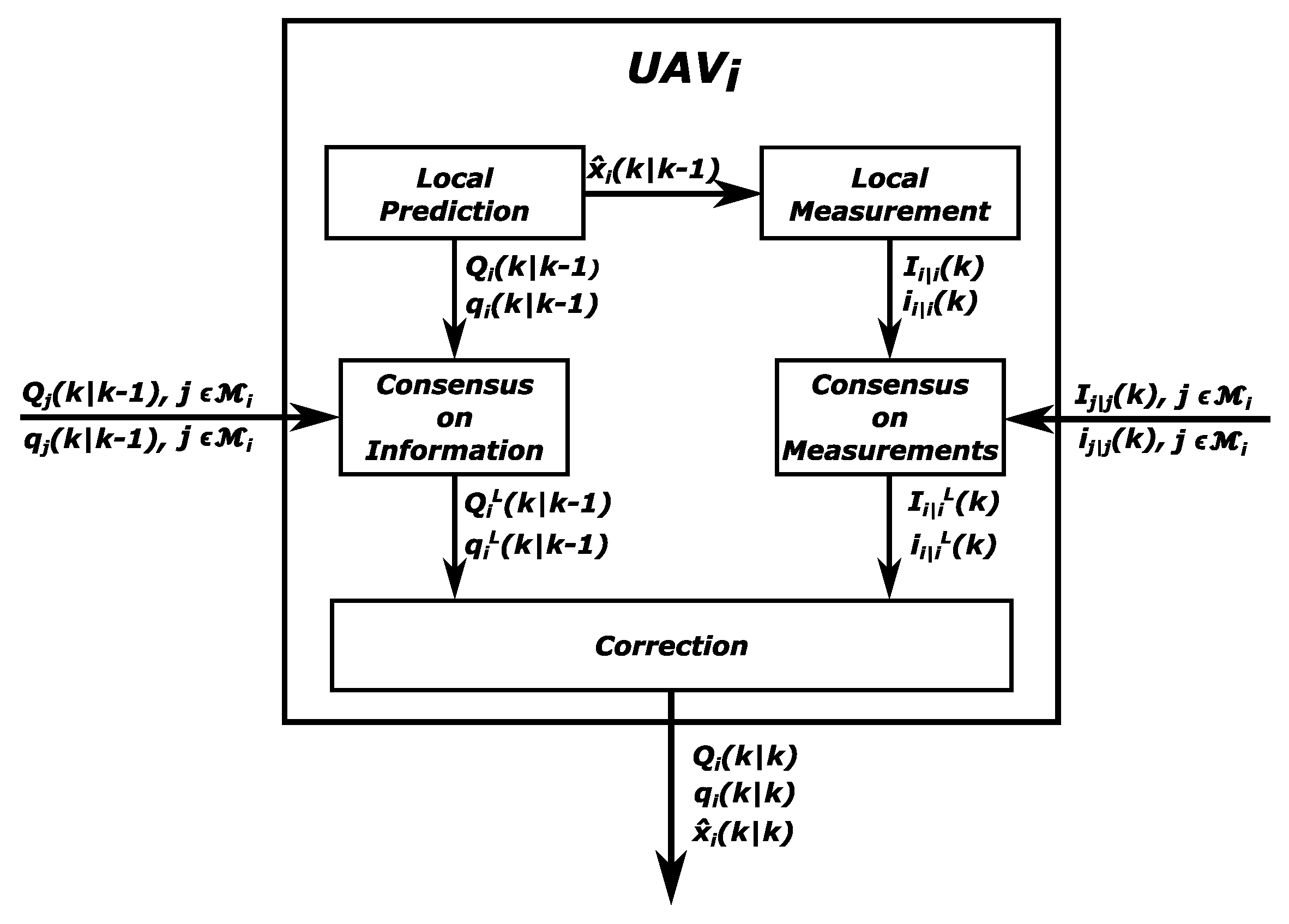
A representation of the algorithm flow and the relationship among phases can be seen in Figure 1.

4. Numerical Simulations

To assess the performance of the proposed algorithm, five simulation tests were conducted with formations of UAVs flying over a designated area of interest. The first simulation test involved a sensitivity analysis to evaluate the impact of key operational parameters, such as the number of consensus iterations L and the communication link schemes $\mathcal{A}$, on situational awareness. The second simulation test examined the algorithm resilience by introducing communication disruptions among certain UAVs, demonstrating its ability to resume estimation once communication was reestablished. The third simulation assessed the algorithm performance in estimating the position of a stationary target within the operational scenario. The fourth example explored the robustness of the algorithm to communication delays. Finally, the fifth test case examined the capability of the algorithm to be integrated in a complete guidance, navigation and control algorithm and involved in a realistic post-avalanche scenario. Additionally, a centralized EKF was employed as a benchmark to compare the performance trade-off between centralized and decentralized techniques.

The numerical simulations presented in this study were conducted using MATLAB routines with a time step size of $T_s=1$ s. Initially, each aircraft knows only its own position information, and the overall state estimate was initialized with random values. This assumption allowed for the evaluation of algorithm convergence towards the correct estimate and the assessment of its ability to achieve consensus.

To take into account measurement errors, they were simulated by introducing biases and white Gaussian noise into the simulation output. The main parameters are summarized in

Table 1. Sensor biases and measurement noise covariance matrices considered in the simulations.

Description	Value
GPS bias—(m)	${[2,2,4]}^T$
Transponder bias—$\left(\mathrm{m}\right)$	$4·{10}^{-2}$
GPS noise covariance—$\left({\mathrm{m}}^2\right)$	${\mathit{I}}_3·{[4·{10}^{-1},4·{10}^{-1},1]}^T$
Transponder noise covariance—$\left({\mathrm{m}}^2\right)$	$1·{\mathit{I}}_{10}·{10}^{-4}$

.

In order to evaluate the performance of the proposed algorithm, two indicators were defined: standard deviation (SD) and mean absolute error (MAE) [41]. The estimation error made by the i-th UAV, relative to the position of the j-th agent at the time instant k, is:

$$e_i^{{\mathit{S}}_j}\left(k\right)=∥{\hat{\mathit{S}}}_{i,j}\left(k\right)-{\mathit{S}}_j\left(k\right)∥$$

(47)

where ${\hat{\mathit{S}}}_{i,j}\left(k\right)$ indicates the position of the j-th agent estimated by the aircraft i The average error in a time window composed by $n_k$ time steps is

$${\mu }_i^{{\mathit{S}}_j}=\frac{1}{n_k}\sum _{k=1}^{n_k}{e}_i^{{\mathit{S}}_j}\left(k\right)$$

(48)

The mean absolute error $MA{E}_i^{{\mathit{S}}_j}$ made by the i-th UAV is defined as follows:

$$MA{E}_i^{{\mathit{S}}_j}=\frac{1}{n_k}\sum _{k=1}^{n_k}{e}_i^{{\mathit{S}}_j}\left(k\right)$$

(49)

Similarly, it is possible to define the standard deviation ${\sigma }_i^{{\mathit{S}}_j}$ with respect to the average error as follows:

$${\sigma }_i^{{\mathit{S}}_j}=\sqrt{\frac{1}{(n_k-1)}\sum _{k=1}^{n_k}{\left(e_i^{{\mathit{S}}_j}\left(k\right)-{\mu }_i^{{\mathit{S}}_j}\right)}^2}$$

(50)

4.1. Simulation Test #1

Simulation test #1 presents the outcomes of a preliminary sensitivity analysis aimed at examining the impact of key operational parameters, specifically the number of consensus steps L and the communication link schemes $\mathcal{A}$, on the performance of the proposed algorithm.

As an illustrative scenario, consider a swarm of 10 UAVs with their initial positions summarized in

Table 2. Simulation Tests #1 and #2—UAVs initial position.

Agent	$\mathit{X}\mathbf{\left(}\mathbf{0}\mathbf{\right)}\mathbf{\left(}\mathbf{m}\mathbf{\right)}$	$\mathit{Y}\mathbf{\left(}\mathbf{0}\mathbf{\right)}\mathbf{\left(}\mathbf{m}\mathbf{\right)}$	$\mathit{Z}\mathbf{\left(}\mathbf{0}\mathbf{\right)}\mathbf{\left(}\mathbf{m}\mathbf{\right)}$
$UA{V}_1$	100	170	100
$UA{V}_2$	100	130	100
$UA{V}_3$	50	100	100
$UA{V}_4$	0	50	100
$UA{V}_5$	−50	100	100
$UA{V}_6$	−100	130	100
$UA{V}_7$	−100	170	100
$UA{V}_8$	−50	200	100
$UA{V}_9$	0	250	100
$UA{V}_{10}$	50	200	100

. Assume that all UAVs in the swarm fly in the same direction at a constant speed of 2 m/s, maintaining a fixed altitude of 100 m above the terrain. Throughout the flight, several maneuvers are performed in both the horizontal and vertical planes, involving changes in altitude. These maneuvers enable the evaluation of the navigation algorithm capability to estimate trajectory modifications.

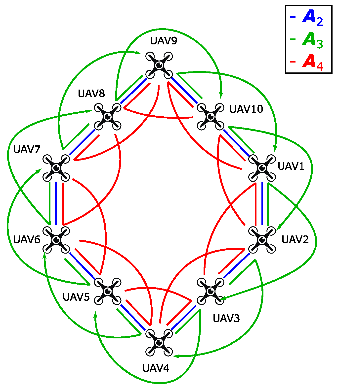
The sensitivity analysis was conducted by considering four distinct configurations of consensus steps, namely $L\in \{3,5,10,20\}$, and three communication schemes (${\mathcal{A}}_2$, ${\mathcal{A}}_3$, ${\mathcal{A}}_4$), characterized by an increasing number of communication links (refer to Figure 2).

As a representative result,

Table 3. Simulation Test #1—Comparison of standard deviation ${\sigma }_1^{S_2}$ of $UA{V}_2$ position estimation error made by $UA{V}_1$ with respect to the number of consensus iterations and communication link schemes.

Communication Scheme $\mathcal{A}$	${\mathit{\sigma }}_{\mathbf{1}}^{{\mathit{S}}_{\mathbf{2}}}$ for $\mathit{L}\mathbf{=}\mathbf{3}$	${\mathit{\sigma }}_{\mathbf{1}}^{{\mathit{S}}_{\mathbf{2}}}$ for $\mathit{L}\mathbf{=}\mathbf{5}$	${\mathit{\sigma }}_{\mathbf{1}}^{{\mathit{S}}_{\mathbf{2}}}$ for $\mathit{L}\mathbf{=}\mathbf{10}$
${\mathcal{A}}_2$	1.0437	1.0418	1.0440
${\mathcal{A}}_3$	0.9669	0.9631	0.9605
${\mathcal{A}}_4$	0.7334	0.7304	0.7294

and

Table 4. Simulation Test #1—Comparison of Mean Absolute Error $MA{E}_1^{S_2}$ of $UA{V}_2$ position estimation made by $UA{V}_1$ with respect to the number of consensus iterations and communication link schemes.

Communication Scheme $\mathcal{A}$	${\mathit{MAE}}_{\mathbf{1}}^{{\mathit{S}}_{\mathbf{2}}}$ for $\mathit{L}\mathbf{=}\mathbf{3}$	${\mathit{MAE}}_{\mathbf{1}}^{{\mathit{S}}_{\mathbf{2}}}$ for $\mathit{L}\mathbf{=}\mathbf{5}$	${\mathit{MAE}}_{\mathbf{1}}^{{\mathit{S}}_{\mathbf{2}}}$ for $\mathit{L}\mathbf{=}\mathbf{10}$
${\mathcal{A}}_2$	0.1781	0.1788	0.1793
${\mathcal{A}}_3$	0.1597	0.1609	0.1611
${\mathcal{A}}_4$	0.1112	0.1099	0.1094

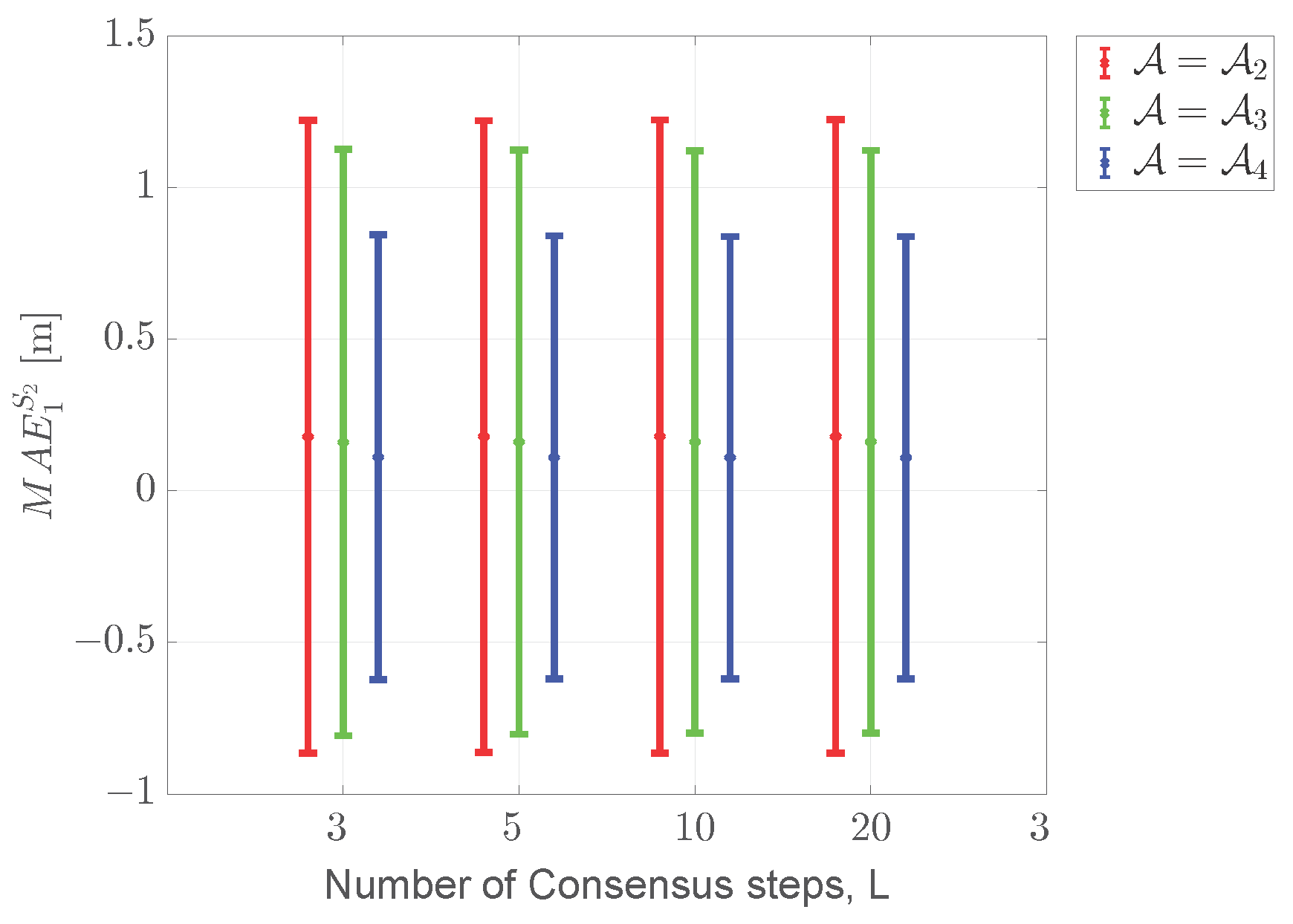
present the standard deviation (54) and the mean absolute error (MAE) (53) of the estimated position of $UA{V}_2$ performed by $UA{V}_1$. These results provide insights into the influence of consensus steps and communication links on the estimation process. It is observed that performance improvement is not consistently achieved by increasing the parameter value. Notably, a higher number of communication links among UAVs leads to better performance, indicated by lower values of standard deviation and mean absolute error, and exhibits limited sensitivity to an increase in consensus steps. This characteristic of the algorithm is further depicted in Figure 3, which visually illustrates the findings from the analysis of Table 3 and Table 4.

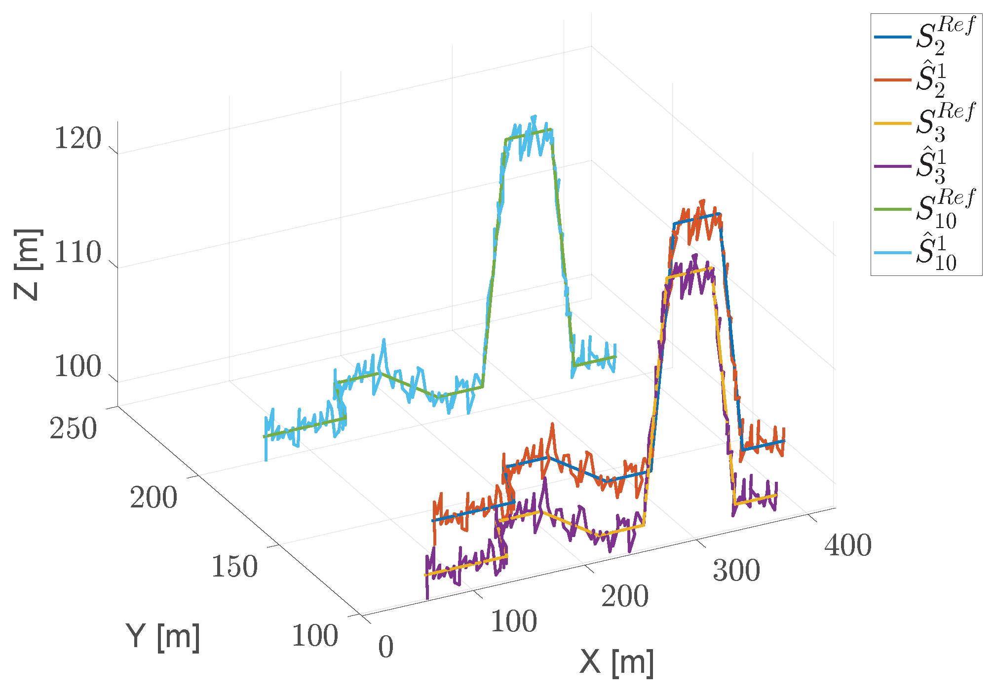
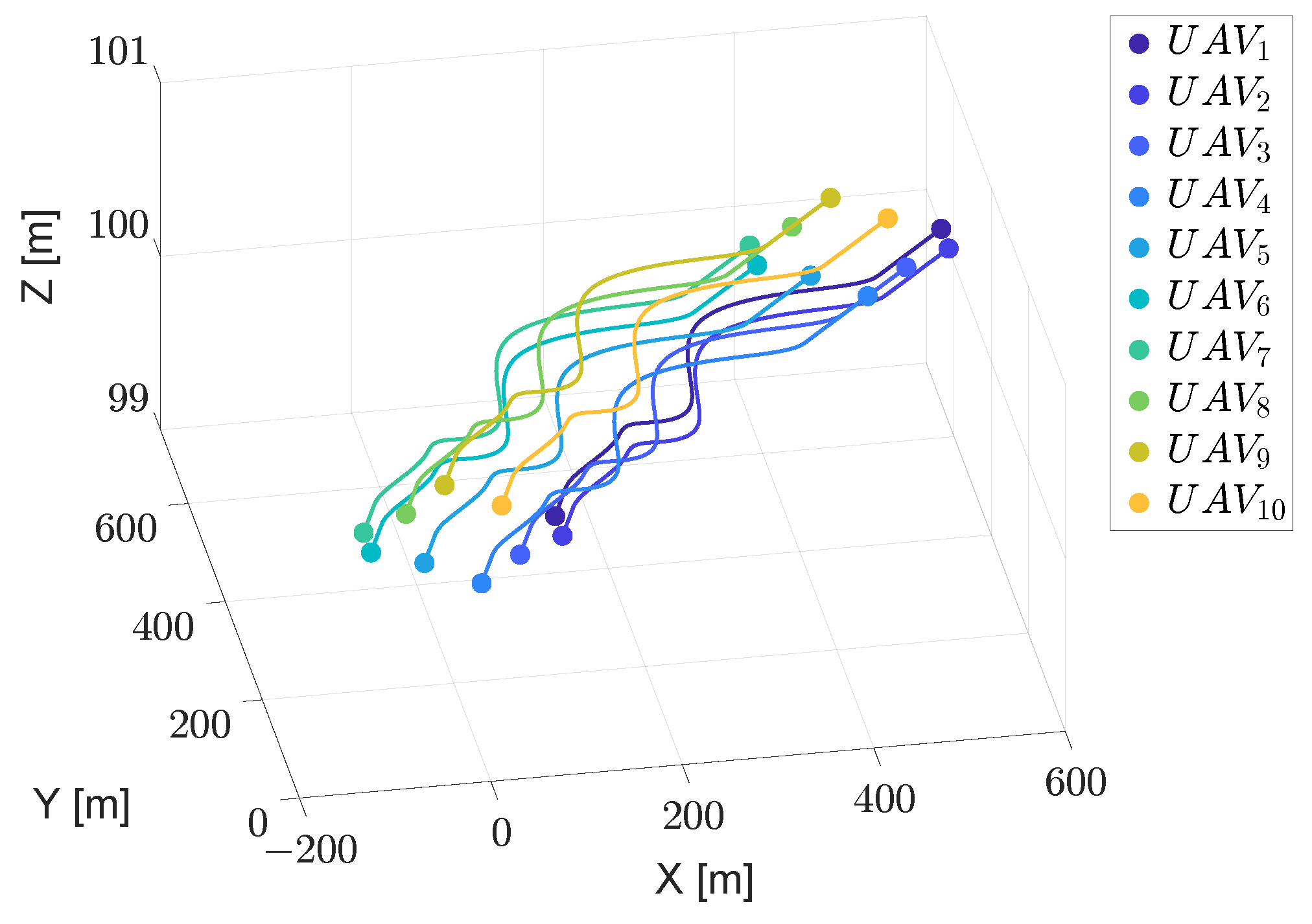
Figure 4 presents an example of the estimated trajectory of UAVs as viewed from $UA{V}_1$ compared with reference trajectories. In this example, with an arbitrary communication configuration $\mathcal{A}=\mathcal{A}3$ and $L=10$, only $UA{V}_2$, $UA{V}_3$ and $UAV{}_{10}$ are visible from $UA{V}_1$, as indicated in Figure 2. Despite the presence of maneuvers, each agent is capable of estimating the positions of the visible UAVs. Specifically, the scenario includes left/right turn maneuvers in the horizontal plane at $t=40$ s and $t=80$ s, followed by pull up/pull down maneuvers in the vertical plane at $t=120$ s and $t=140$ s.

4.2. Simulation Test #2

For simulation test #2, consider the same scenario with 10 UAVs as in simulation test #1. The UAVs start from the initial positions specified in Table 2 and fly in the same direction at a constant speed of 2 m/s, maintaining a fixed altitude of 100 m above the terrain. The trajectories of the UAVs, depicted in Figure 5, include several maneuvers in the horizontal plane before reaching the destination point.

The primary objective of simulation test #2 is to evaluate the algorithm capability to resume trajectory estimation for UAVs following communication interruptions among the aircraft. To illustrate such a feature, the proposed scenario introduces communication link failures during the flight due to obstacle avoidance. Specifically, at two specified time intervals, $t_1=65$ s and $t_2=120$ s, lasting $\mathrm{\Delta }t=10$ s, the communication links among UAVs are disrupted. The affected aircraft include $UA{V}_1$, $UA{V}_2$, $UA{V}_6$ and $UA{V}_7$. 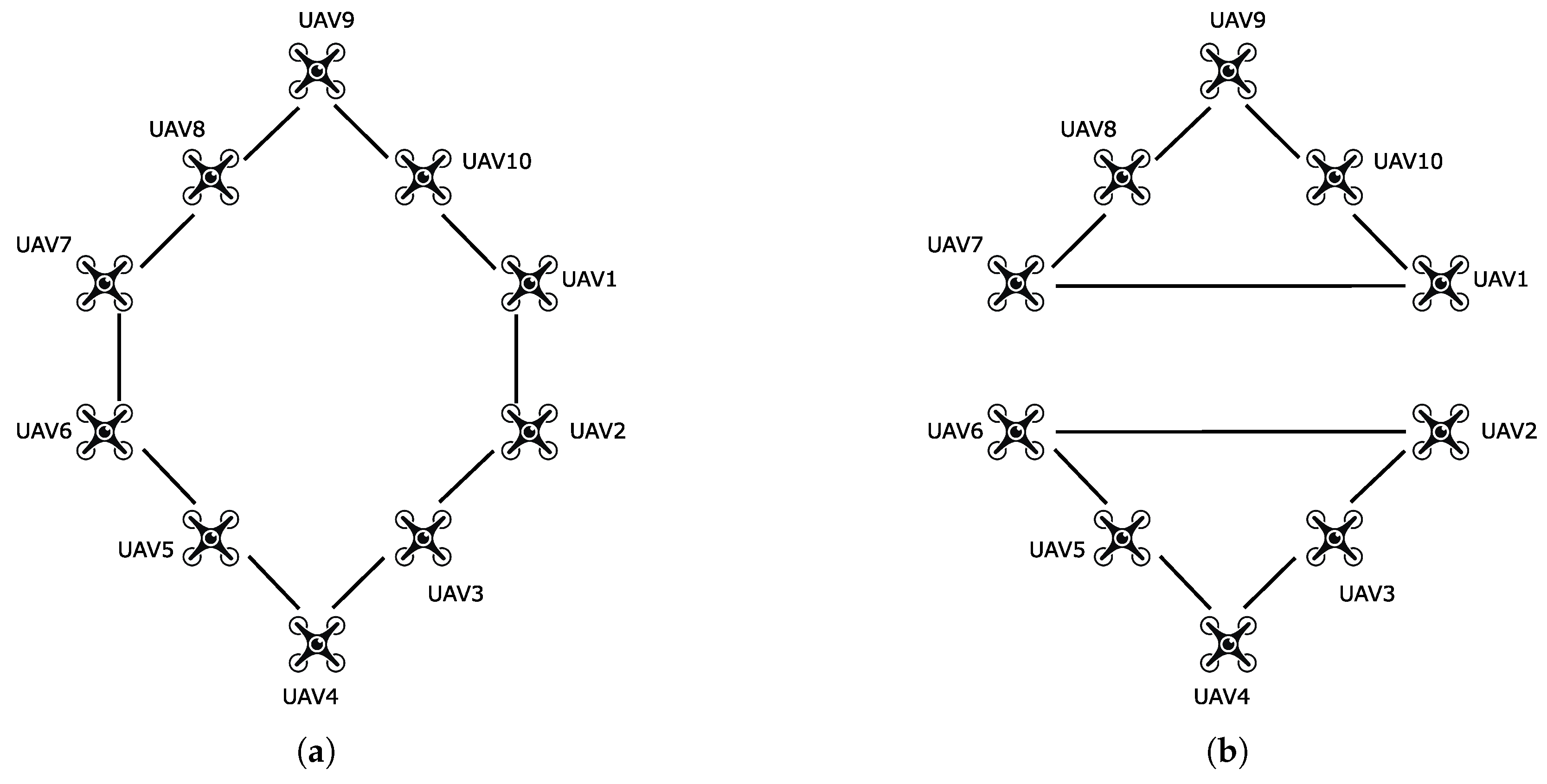Figure 6 displays the communication links before and after the interruptions, highlighting the formation of two sub-swarms. When the data transmission between $UA{V}_1$ and $UA{V}_2$, as well as between $UA{V}_6$ and $UA{V}_7$, is lost, the two sub-swarms reorganize into separate cycle graphs to accurately estimate the state of their neighboring UAVs [42,43].

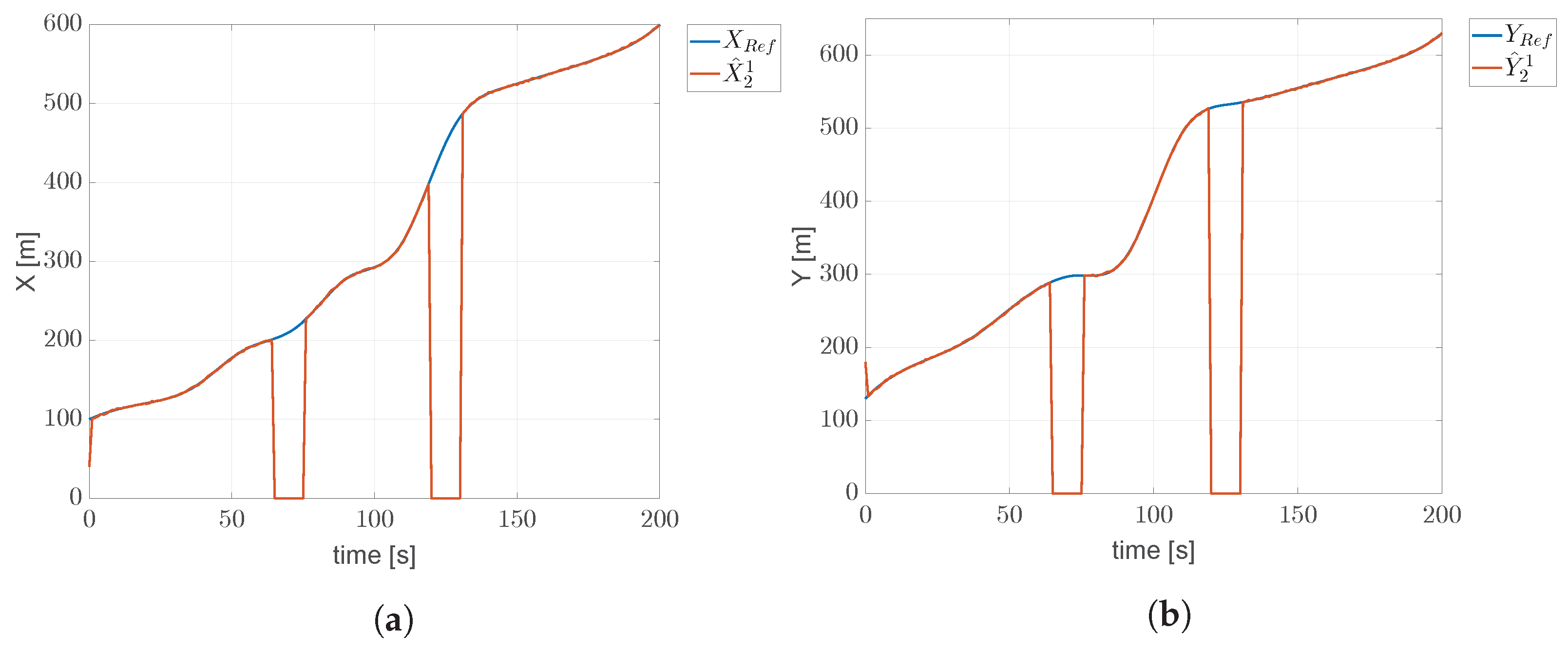
Figure 7 depicts the estimated coordinates of $UA{V}_2$ by $UA{V}_1$ compared with the reference trajectory. As observed in the figure, the position estimation made by $UA{V}_1$ is interrupted solely during the two designated time intervals of communication loss, and it is promptly resumed once the connection among the aircraft is re-established.

4.3. Simulation Test #3

Simulation test #3 aims to evaluate the navigation algorithm ability to estimate the position of a stationary target within the operational scenario. To validate its estimation performance, a comparison was conducted with a centralized version of the KF.

In this test, a sample scenario was considered, involving a formation of 10 UAVs flying together to survey the area of interest and locate the target. Each aircraft maintains a constant speed of 2 m/s, flying in the same direction at an altitude of 100 m above the terrain. Communication capabilities are limited to two neighboring agents, forming a cycle graph, while each UAV is equipped with an additional receiver to detect the signal emitted by the target within a range of $d_{sens}=200$ m. To account for the noise in the target transmitter signal, the simulation parameters outlined in Table 1 are augmented with the bias and noise covariance values specified in

Table 5. Simulation Test #3—Target transceiver parameters in terms of bias and noise covariance.

Description	Value
Target transmitter bias—(m)	$4·{10}^{-4}$
Target transmitter noise covariance—$\left({\mathrm{m}}^2\right)$	$1·{\mathit{I}}_1·{10}^{-4}$

.

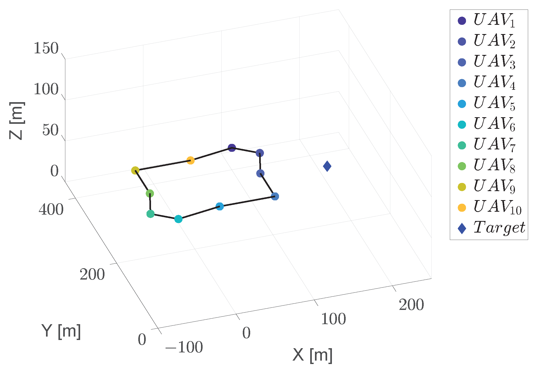
The aircraft navigate towards the target position located at $(212.1,362.1,0)$ m, starting from their respective initial positions as presented in

Table 6. Simulation Test #3—UAVs starting position.

Agent	$\mathit{X}\mathbf{\left(}\mathbf{0}\mathbf{\right)}\mathbf{\left(}\mathbf{m}\mathbf{\right)}$	$\mathit{Y}\mathbf{\left(}\mathbf{0}\mathbf{\right)}\mathbf{\left(}\mathbf{m}\mathbf{\right)}$	$\mathit{Z}\mathbf{\left(}\mathbf{0}\mathbf{\right)}\mathbf{\left(}\mathbf{m}\mathbf{\right)}$
$UA{V}_1$	56.6	234.8	100
$UA{V}_2$	84.8	206.6	100
$UA{V}_3$	70.7	150	100
$UA{V}_4$	70.7	79.3	100
$UA{V}_5$	0	79.3	100
$UA{V}_6$	−56.6	65.1	100
$UA{V}_7$	−84.8	93.4	100
$UA{V}_8$	−70.7	150	100
$UA{V}_9$	−70.7	220.7	100
$UA{V}_{10}$	0	220.7	100

and Figure 8.

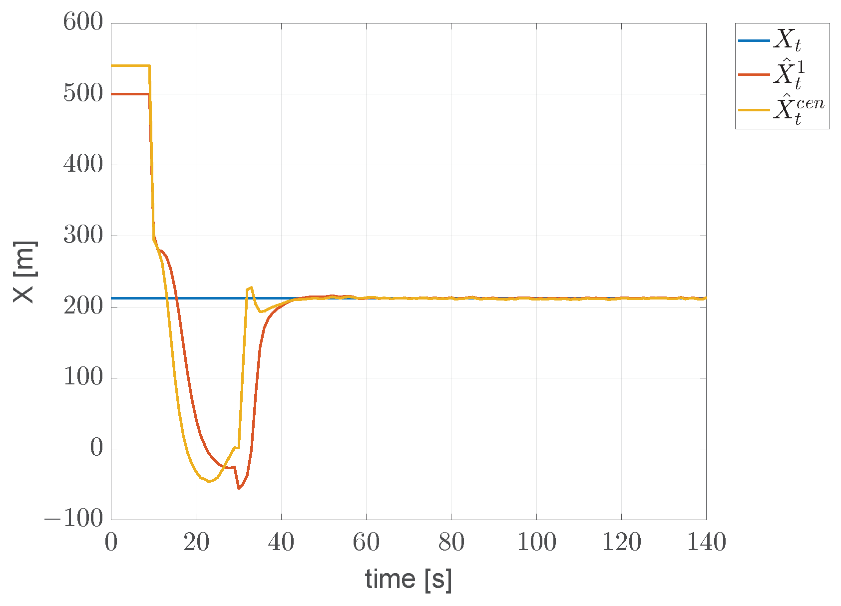
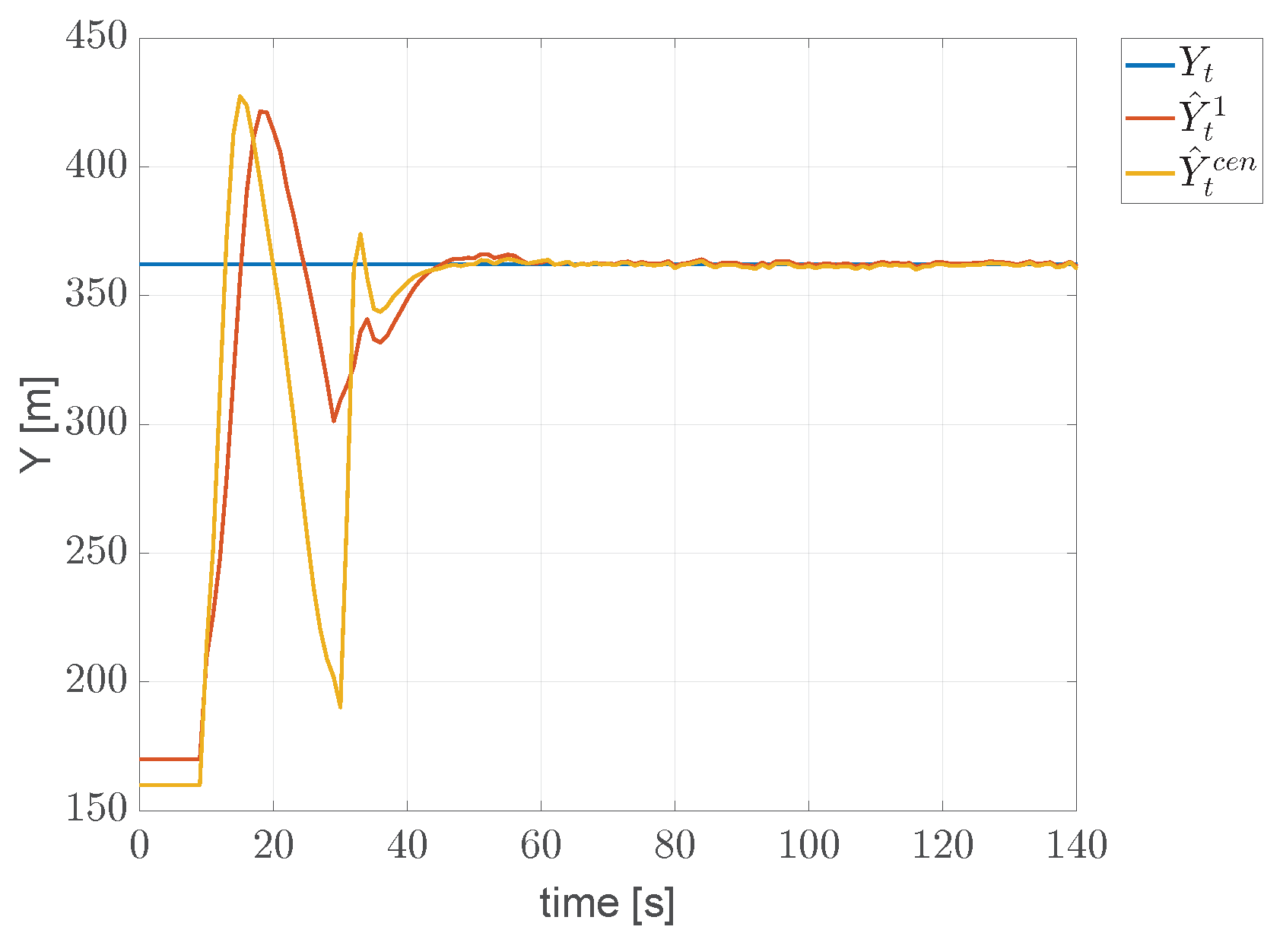
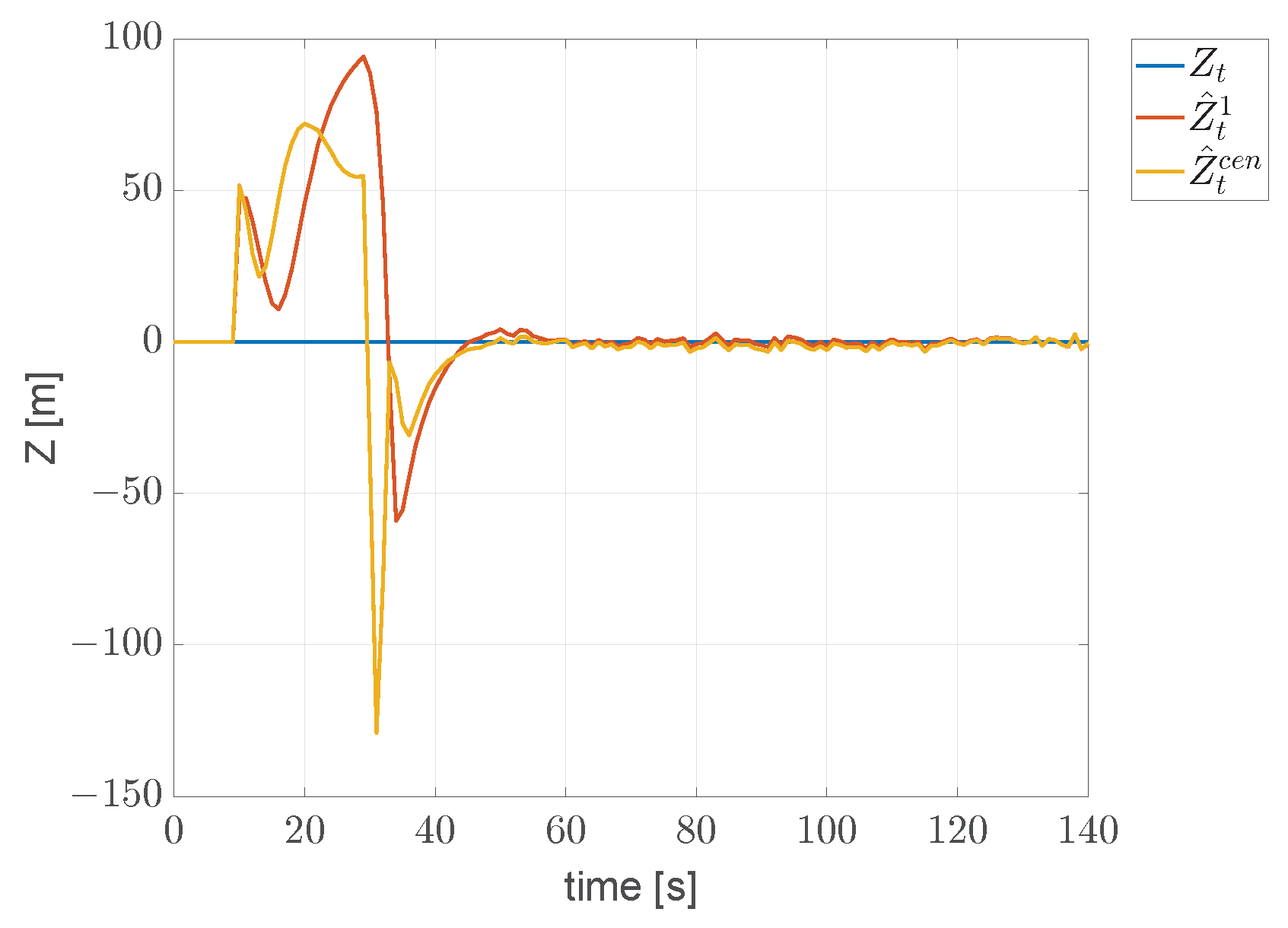
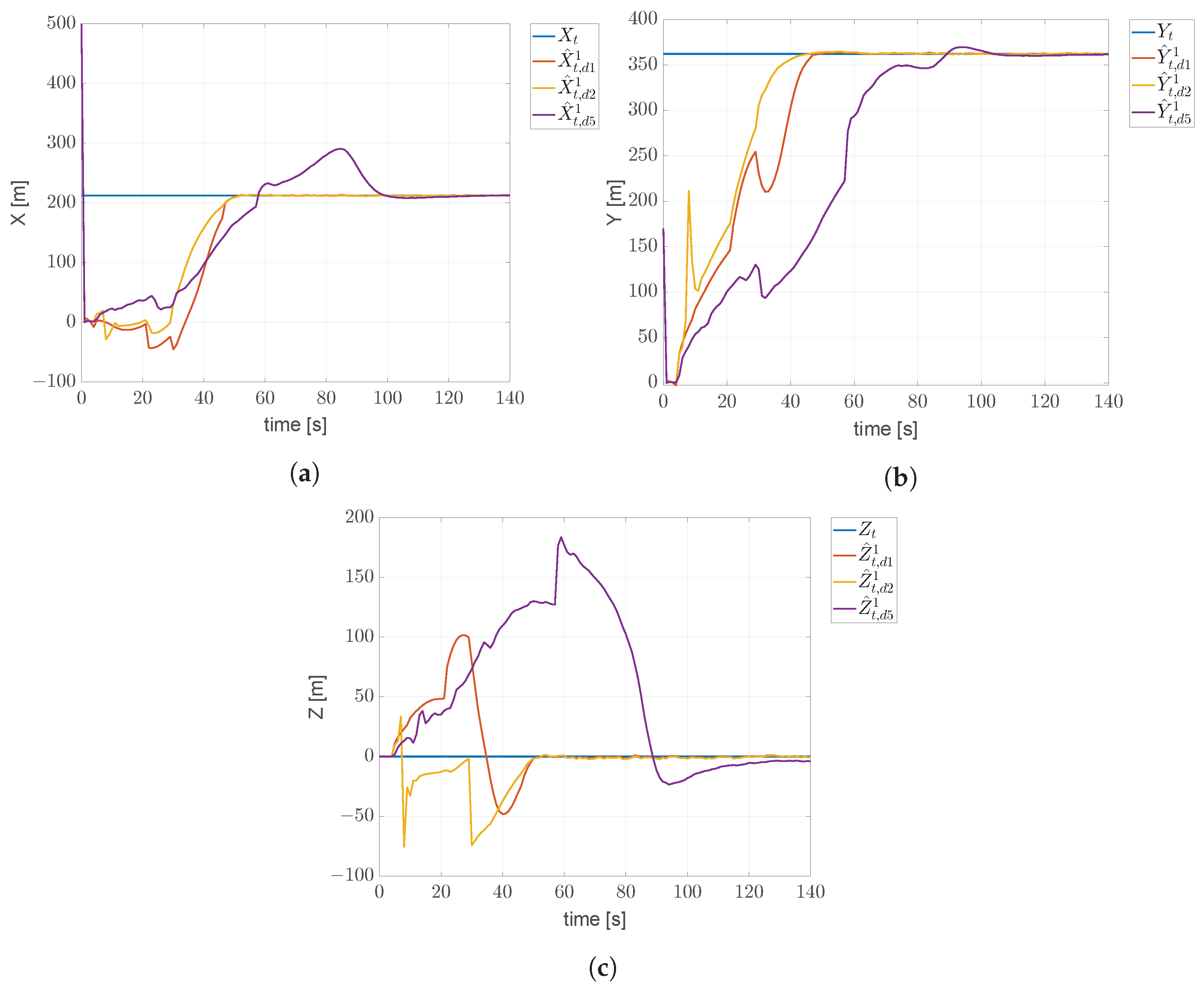
Figure 9, Figure 10 and Figure 11 depict the estimated components of the target position vector, providing a comparison among the actual value, the estimation obtained from the centralized KF and that derived from the proposed decentralized KF. As observed in the figures, during the initial phase of the simulation, the target position remains unknown as it lies outside the sensor range of the UAVs.

At $t=10$ s, the target enters the sensor range of $UA{V}_1$, but localization is not yet feasible. It is worth noting that for localization problems based on fusion algorithms, a minimum of three aircraft measurements is required to accurately determine the target location [44,45,46].

From $t=30$ s, the target comes within the sensor range of $UA{V}_1$, $UA{V}_2$, $UA{V}_3$ and $UA{V}_{10}$, thus becoming localizable.

The estimated target position definitively converges around $t=43$ s.

The estimation error made by the i-th UAV, relative to the position of the target at the time instant k, is:

$$e_i^{\eta }\left(k\right)=∥{\hat{\eta }}_i\left(k\right)-\eta \left(k\right)∥$$

(51)

where ${\hat{\eta }}_i\left(k\right)$ indicates the position component of the target estimated by the aircraft i. The average error in a time window composed by $n_k$ time steps is

$${\mu }_i^{\eta }=\frac{1}{n_k}\sum _{k=1}^{n_k}{e}_i^{\eta }\left(k\right)$$

(52)

The mean absolute error $MA{E}_i^{\eta }$ made by the i-th UAV is defined as follows:

$$MA{E}_i^{\eta }=\frac{1}{n_k}\sum _{k=1}^{n_k}{e}_i^{\eta }\left(k\right)$$

(53)

Similarly, it is possible to define the standard deviation ${\sigma }_i^{\eta }$ with respect to the average error as follows:

$${\sigma }_i^{\eta }=\sqrt{\frac{1}{(n_k-1)}\sum _{k=1}^{n_k}{\left(e_i^{\eta }\left(k\right)-{\mu }_i^{\eta }\right)}^2}$$

(54)

Table 7. Simulation Test #3—Results comparison in terms of standard deviation and Mean Absolute Error.

Performance Index	Proposed HCMCI Model	Centralized Model
${\sigma }_1^{X_t}\left(\mathrm{m}\right)$	0.6250	0.6251
${\sigma }_1^{Y_t}\left(\mathrm{m}\right)$	0.5972	0.6223
${\sigma }_1^{Z_t}\left(\mathrm{m}\right)$	1.0847	0.7911
$MA{E}_1^{X_t}\left(\mathrm{m}\right)$	0.2013	0.1515
$MA{E}_1^{Y_t}\left(\mathrm{m}\right)$	0.2839	0.1586
$MA{E}_1^{Z_t}\left(\mathrm{m}\right)$	0.0438	0.1851

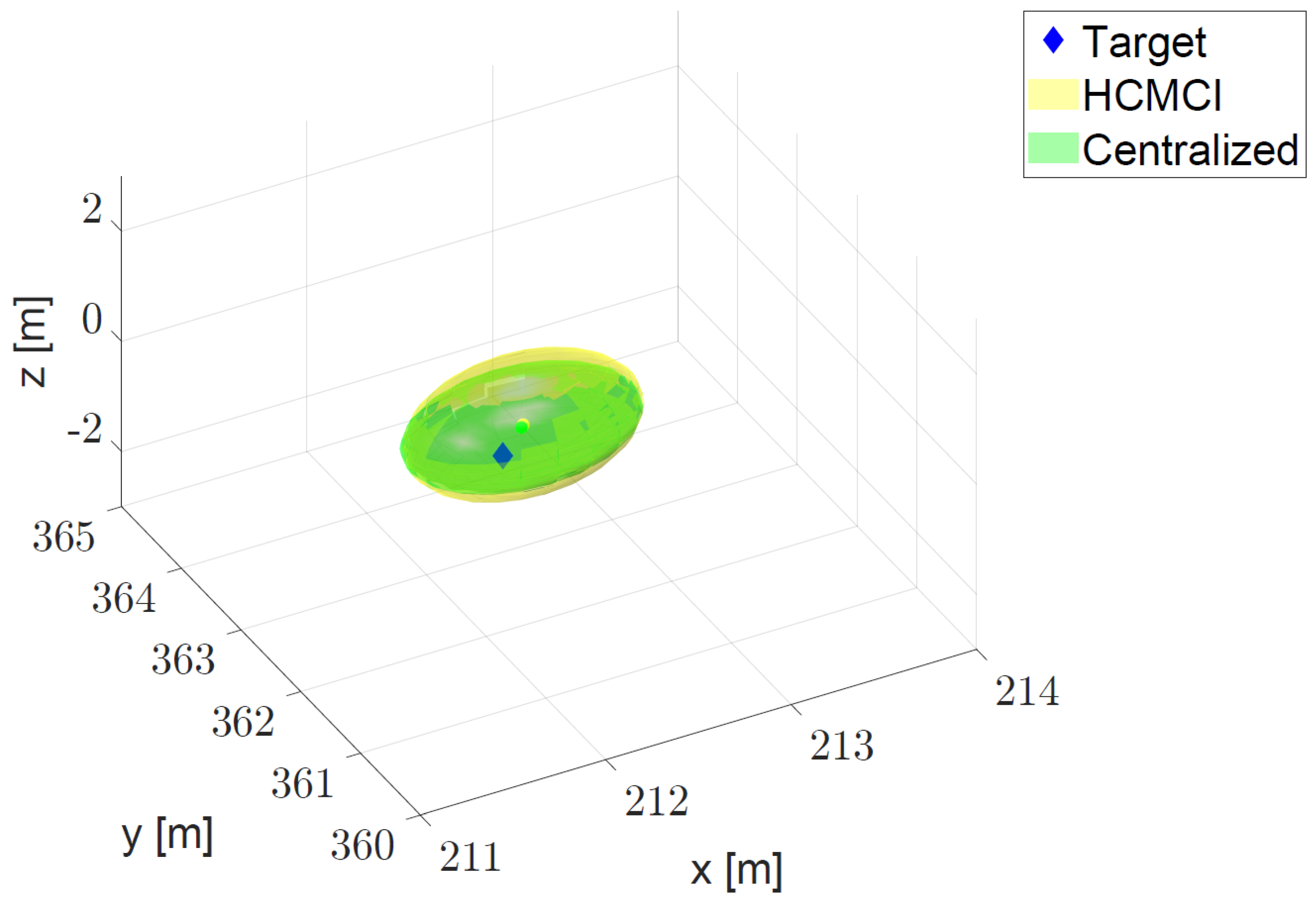
shows mean absolute error and standard deviation computed by UAVs for any component $\eta$ of the target position vector.

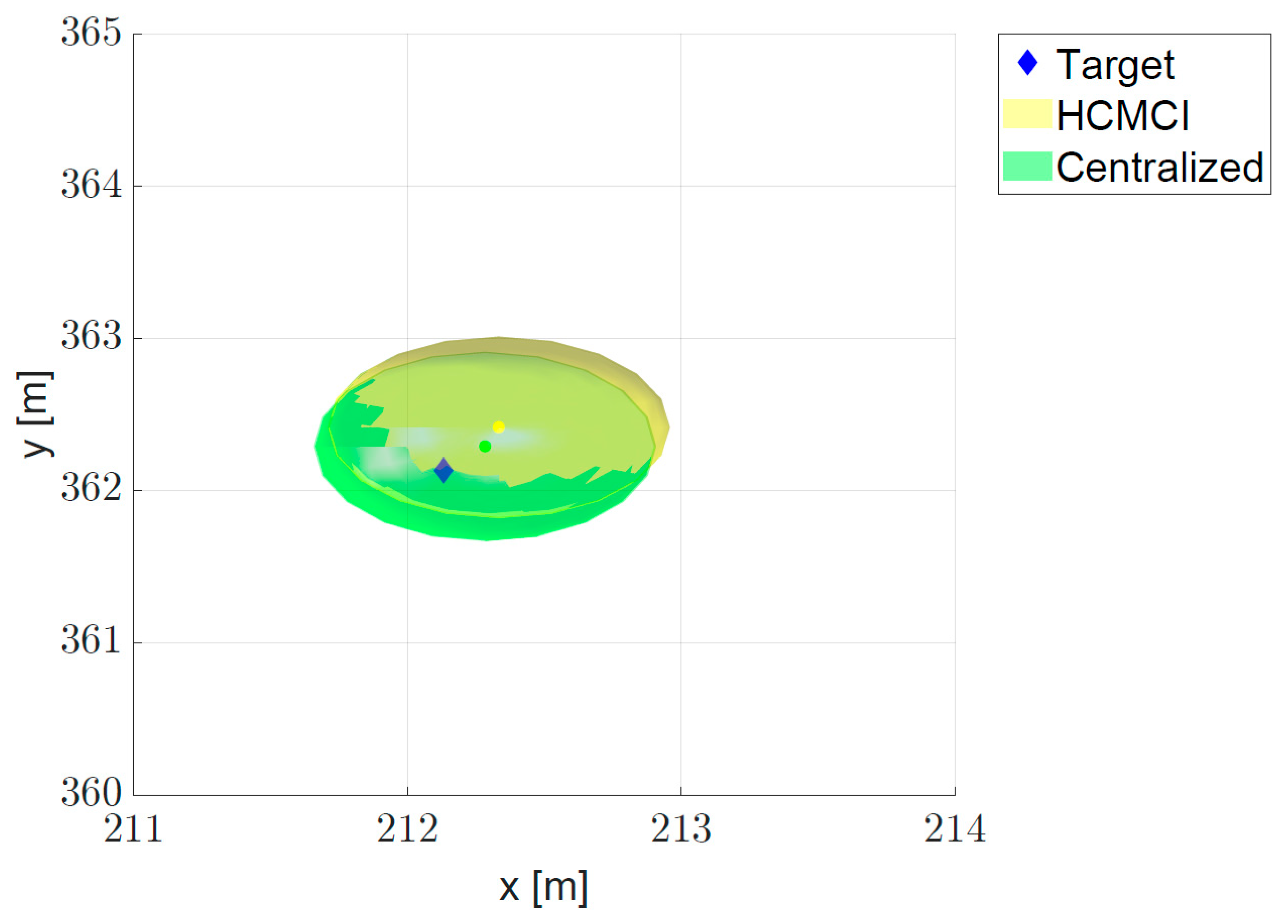
Figure 12 and Figure 13 show the uncertain target volume detected by the proposed algorithm with respect to the centralized KF and the real target position.

4.4. Simulation Test #4

Simulation test #4 aims to assess the navigation algorithm’s capability to estimate the position of a stationary target within the operational scenario in the presence of communication delays among the swarm of UAVs. The same scenario shown in the previous subsection was considered (see Table 6), where the communication channel among UAVs is not considered ideal but introduces a delay typical of wireless communication.

Considering the size of UAVs and the typical size of the considered scenarios, three different constant communication delays among aircraft in the formation were considered, $0.1$ s, $0.2$ s and $0.5$ s, to stress the procedure in the worst situations.

As already shown, results do not depend on the number of consensus steps when $L\ge 3$, while the communication scheme can give a performance improvement.

As a representative result, Figure 14 shows the capability of the algorithm to localize the target also in the configuration $\mathcal{A}={\mathcal{A}}_2$, considered as the worst possible because it shows the slowest convergence in previous results. It is worth noticing that the algorithm is robust to any communication delay until $0.5$ s, with a convergence speed that decreases by increasing the length of the delay. Without delays, the estimation of the target position converges to the real value at $t=43$ s (see Figure 9, Figure 10 and Figure 11), while with a delay of $0.5$ s, the convergence is assured only after $t=110$ s.

4.5. Simulation Test #5, a Post-Avalanche Scenario

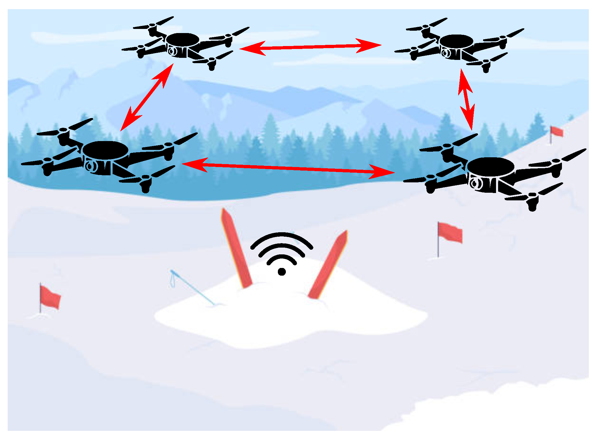
The primary objective of this section is to prove the effectiveness of the proposed navigation algorithm in a SAR mission for locating a missing skier. An illustrative example is shown in Figure 15, where a swarm of UAVs identifies the missing individual, points towards the target and subsequently awaits the rescue phase by hovering over the skier.

To address this issue, consider a swarm of N UAVs flying at a fixed altitude whose guidance algorithm is based on the DTG-based approach [47]. This approach ensures that the the swarm remains distributed and scalable, without a leader–follower architecture, while maintaining a local triangular topology that is highly efficient in terms of the packing problem.

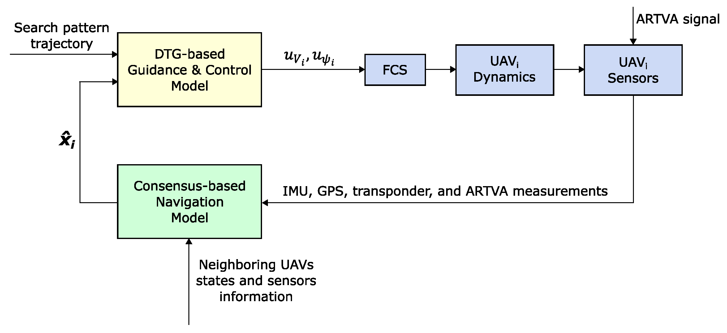
The integrated GNC scheme is depicted in Figure 16, which provides an overview of the overall architecture and the information flow between the high-level DTG-based guidance and control and the consensus-based navigation modules.

The proposed scenario represents a simplified environment with no disturbances, such as wind. It is also assumed that the swarm is homogeneous, consisting of the same type of quadrotors. We have assumed perfect conditions for communication and reconnaissance of the search area. Therefore, no communication delays and no loss of precision over greater distances are considered. Furthermore, the take off and landing of UAVs are not modeled; it is assumed that all UAVs have already been launched at the beginning of the scenario and are flying at a fixed altitude. Battery consumption is not included in the model.

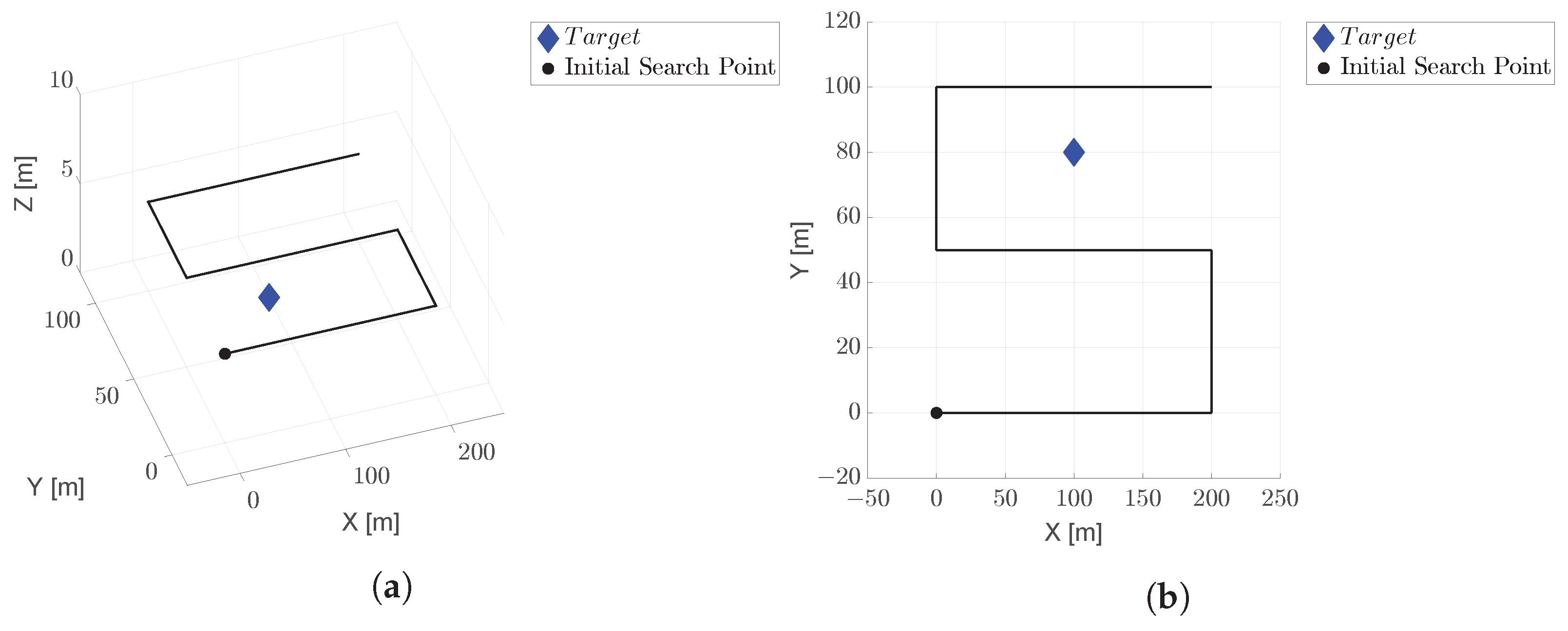
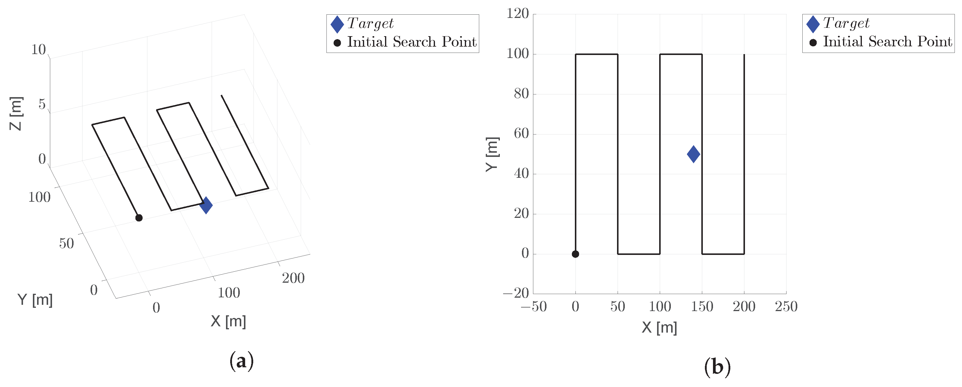
The case study takes into account real research techniques in post avalanche scenarios. The most known search strategies are the parallel track and creeping line search. They involve maintaining parallel tracks, with the former being parallel to the major axes and the latter parallel to the minor axes. These strategies are suitable for uncertain target locations and flat terrain, ensuring uniform coverage.

The typical post-avalanche zones to be surveyed are usually small [48]; in this section, the operational scenarios are defined over an area of $[200\times 100]$ m. Two scenarios are provided, with the same area and different positions of the skier, as summarized in

Table 8. Real position of the Skier.

Scenario ID	Skier Position (m)
1	${\mathit{S}}_s={[100,180,0]}^T$
2	${\mathit{S}}_s={[140,50,0]}^T$

.

Given the search area, a formation of 5 UAVs was deployed, flying at a fixed altitude of 5 m and cruising at a speed of 3 m/s.

To cover the selected search area, two coverage techniques were explored, as they are the most suitable for this type of mission: the parallel track technique was used in scenario #1 (Figure 17) and the creeping line in scenario #2 (Figure 18). Both search paths have the same length and guarantee complete surveillance of the defined area.

UAV starting positions for both operational scenarios are given in

Table 9. Simulation Test #5—UAVs Initial position.

Agent	$\mathit{X}\mathbf{\left(}\mathbf{0}\mathbf{\right)}\mathbf{\left(}\mathbf{m}\mathbf{\right)}$	$\mathit{Y}\mathbf{\left(}\mathbf{0}\mathbf{\right)}\mathbf{\left(}\mathbf{m}\mathbf{\right)}$	$\mathit{Z}\mathbf{\left(}\mathbf{0}\mathbf{\right)}\mathbf{\left(}\mathbf{m}\mathbf{\right)}$
$UA{V}_1$	0	0	5
$UA{V}_2$	−20	30	5
$UA{V}_3$	−20	−30	5
$UA{V}_4$	−40	20	5
$UA{V}_5$	−40	−20	5

.

The ARTVA receiver is the device responsible for detecting the presence of the skier under the snow. Its operational range is currently about 60 m [49]. However, although the most modern versions of these devices are valid and efficient, their performance in real operating conditions are degraded due to several factors, like ambient noise and interference with other electronic devices or other beacons. Considering an altitude of 5 m, the projected detection area over the terrain has a diameter of $d_{sens}=20$ m.

Table 10. Simulation Test #5—Sensor biases and measurement noise covariance matrices.

Description	Value
GPS bias—$\left(\mathrm{m}\right)$	${[2,2,4]}^T$
Accelerometer bias—$(\mathrm{m}/{\mathrm{s}}^2)$	${[0.1,0.15,0.2]}^T$
Gyro bias—$(\mathrm{rad}/\mathrm{s})$	${[0.1,0.08,0.11]}^T$
Magnetometer bias—$\left(\mathrm{G}\right)$	${[0.05,0.02,0.06]}^T$
Transponder bias—$\left(\mathrm{m}\right)$	$4·{10}^{-2}$
ARTVA bias—$\left(\mathrm{m}\right)$	$1.2$
GPS noise covariance—$\left({\mathrm{m}}^2\right)$	${\mathit{I}}_3·{[4·{10}^{-1},4·{10}^{-1},1]}^T$
Accelerometer noise covariance—$\left({(\mathrm{m}/{\mathrm{s}}^2)}^2\right)$	$1·{\mathit{I}}_3·{10}^{-4}$
Gyro noise covariance—$\left({(\mathrm{rad}/\mathrm{s})}^2\right)$	$8·{\mathit{I}}_3·{10}^{-8}$
Magnetometer noise covariance—$\left({\mathrm{G}}^2\right)$	$4·{\mathit{I}}_3·{10}^{-8}$
Transponder noise covariance—$\left({\mathrm{m}}^2\right)$	$1·{\mathit{I}}_4·{10}^{-4}$
ARTVA noise covariance—$\left({\mathrm{m}}^2\right)$	$1·{\mathit{I}}_1·{10}^{-1}$

shows the sensor biases and the measurement noise covariance matrices.

At the beginning of the simulation, it is assumed that each UAV knows only its position, initializing the overall state estimate with random values. Such an assumption is useful for evaluating algorithm convergence to the correct estimate and ability to reach the consensus.

The proposed scenarios were simulated in MATLAB routines with a step size of $T_s=0.1$ s, $L=5$ consensus steps and a simulation period of $T=400$ s.

Simulation parameters are presented in

Table 11. Simulation Test #5—Parameters of the integrated GNC model.

Parameter	Value
Cruise speed $V_c$ $(\mathrm{m}/\mathrm{s})$	3
Minimum speed $V_{min}$ $(\mathrm{m}/\mathrm{s})$	0
Maximum speed $V_{max}$ $(\mathrm{m}/\mathrm{s})$	10
Minimum normal acceleration $a_{min}^{\perp }$ $(\mathrm{m}/{\mathrm{s}}^2)$	−5
Maximum normal acceleration $a_{max}^{\perp }$ $(\mathrm{m}/{\mathrm{s}}^2)$	5
Minimum tangential acceleration $a_{min}^{\Vert }$ $(\mathrm{m}/{\mathrm{s}}^2)$	−10
Maximum tangential acceleration $a_{max}^{\Vert }$ $(\mathrm{m}/{\mathrm{s}}^2)$	10
Safety distance $d_{safety}$ $\left(\mathrm{m}\right)$	3
Desired distance $\overline{d}$ $\left(\mathrm{m}\right)$	20
UAV size ${\overline{r}}_j\forall j=1,\dots ,N$ $\left(\mathrm{m}\right)$	1
MPC weight matrix for tracking error ${\mathbf{Q}}_{MPC}$	diag([10,10,10,10])
MPC weight matrix for control effort ${\mathbf{R}}_{MPC}$	diag([1,1])
Number of steps of the MPC prediction horizon $n_p$	10
Number of steps of the MPC control horizon $n_c$	5

.

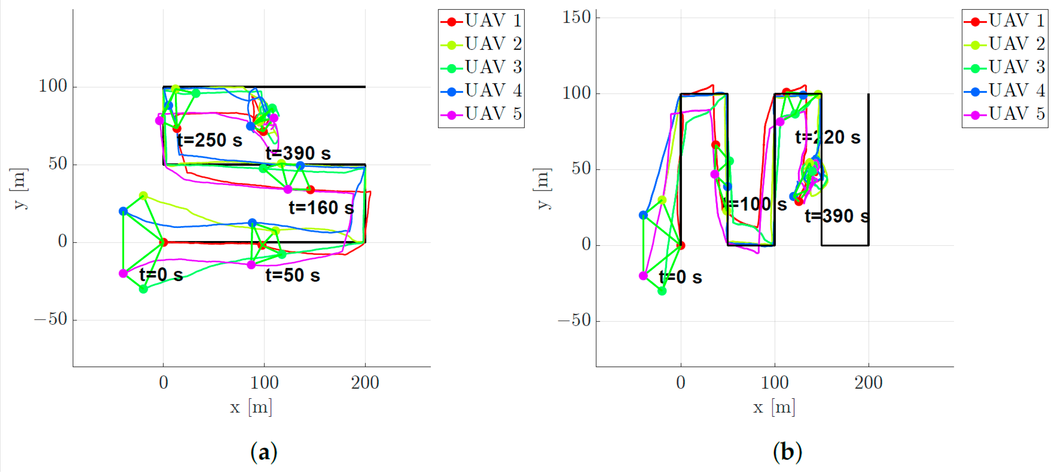
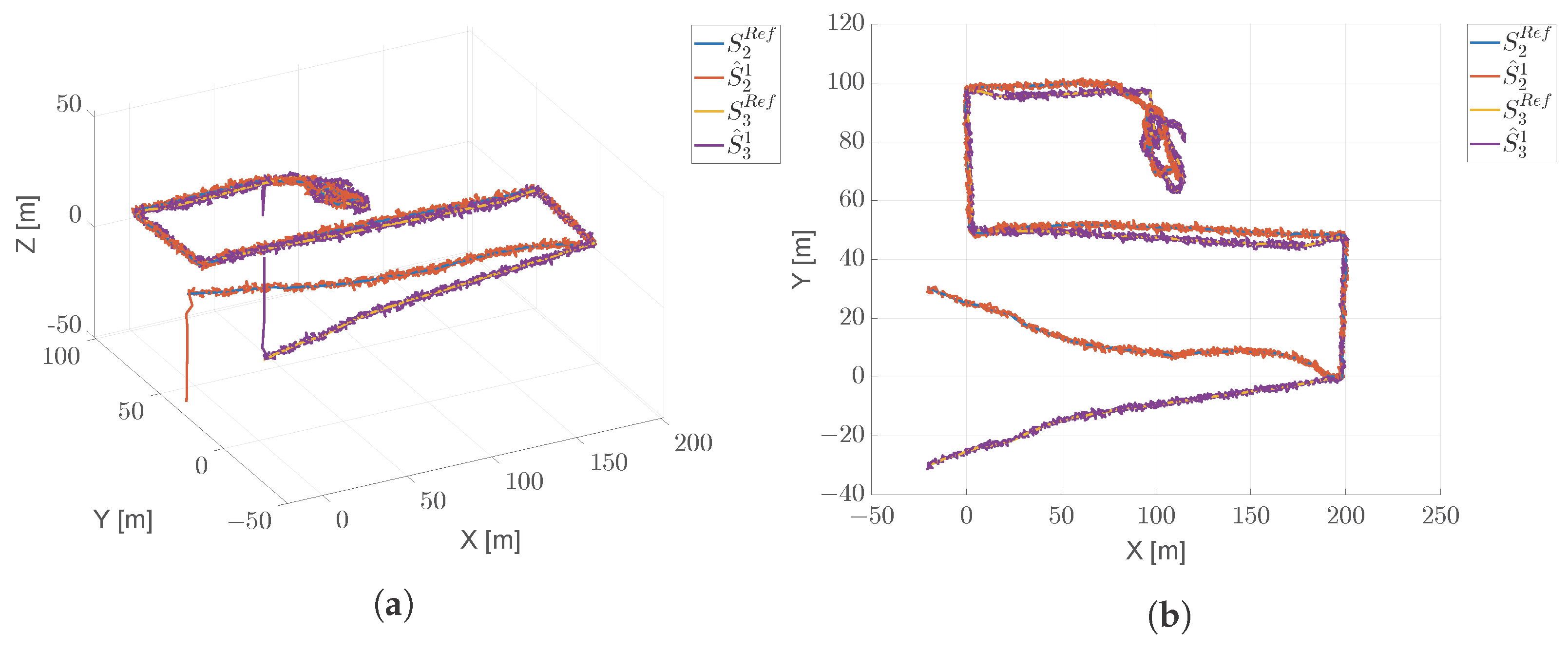
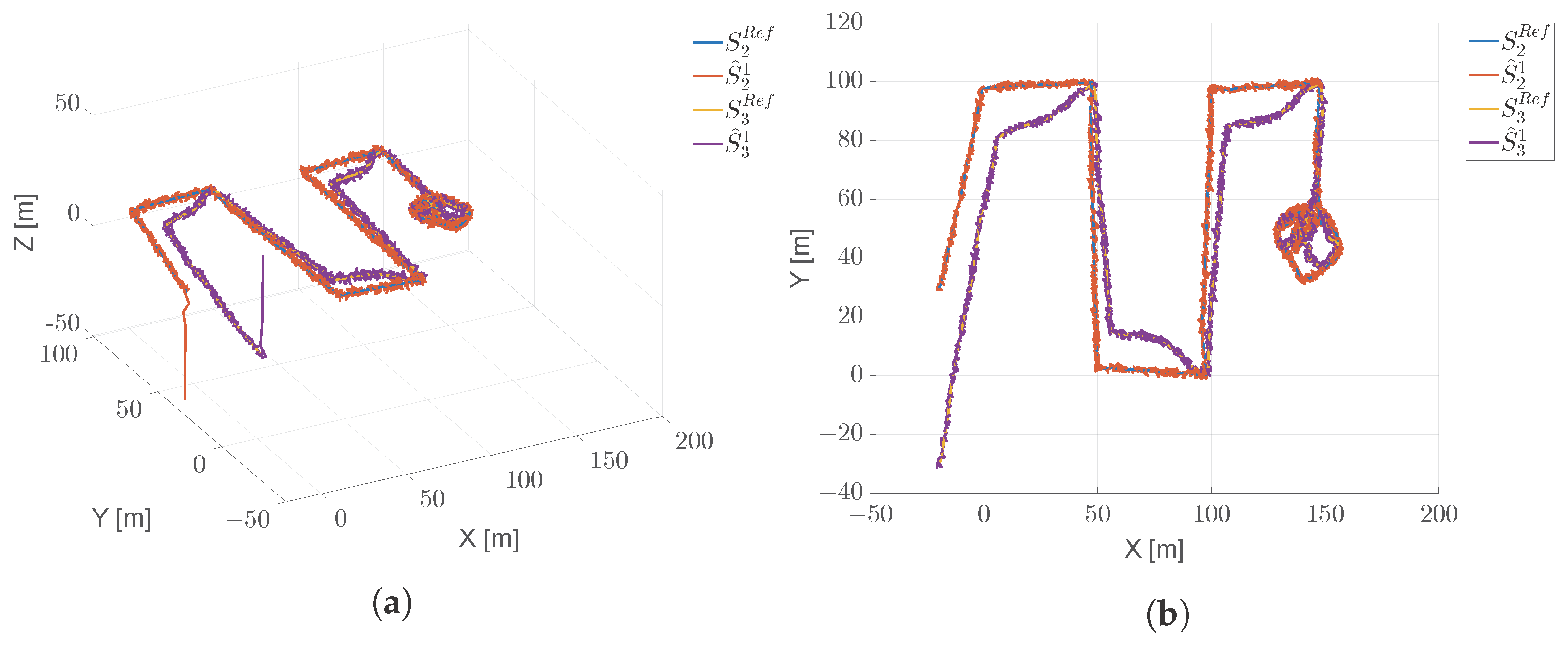
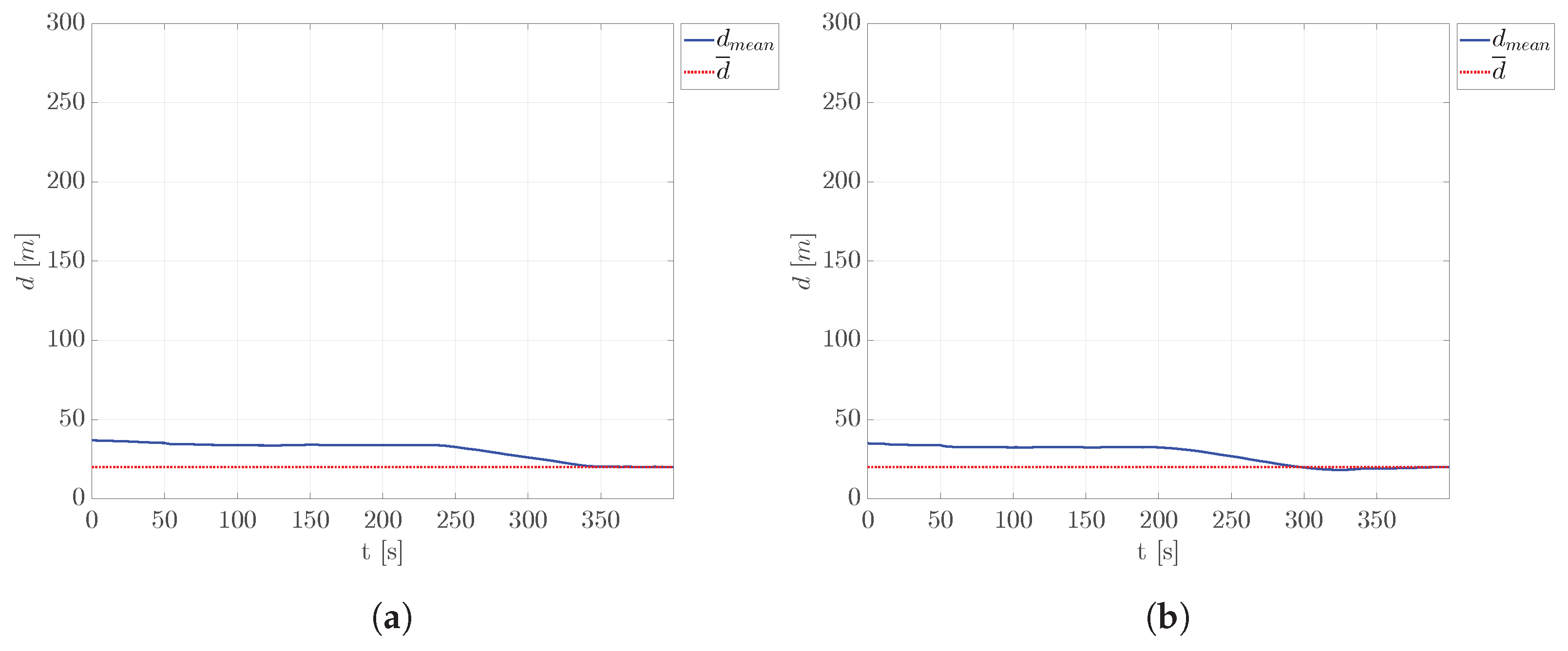
Figure 19 represents the trajectories of the UAV swarm following the parallel track (Figure 19a) and the creeping line (Figure 19b) search patterns. Green solid lines indicate the obtained formation graph. The distance among aircraft tends to remain near the desired value, $\overline{d}$, for all the duration of the simulation and for both the considered research methodologies, as also confirmed by the analysis of Figure 20. The purpose of the swarm is to fly over the area near the missing person, once its position is identified. This behavior is highlighted by the continuous flight above the skier position at $T=390$ s (see Figure 17 and Figure 18), as shown in Figure 19.

Figure 21 and Figure 22 show trajectories of $UA{V}_2$ and $UA{V}_3$ as estimated by $UA{V}_1$, compared with reference paths. As can be seen, $UA{V}_1$ is always able to estimate its neighbors’ trajectories. It is worth remembering that each UAV in the swarm, at the beginning of the simulation, knows only its position, and the estimates start at random values. As can be seen, the estimates made by $UA{V}_1$ converge to the correct values after a few time instants, necessary for the convergence of the consensus algorithm.

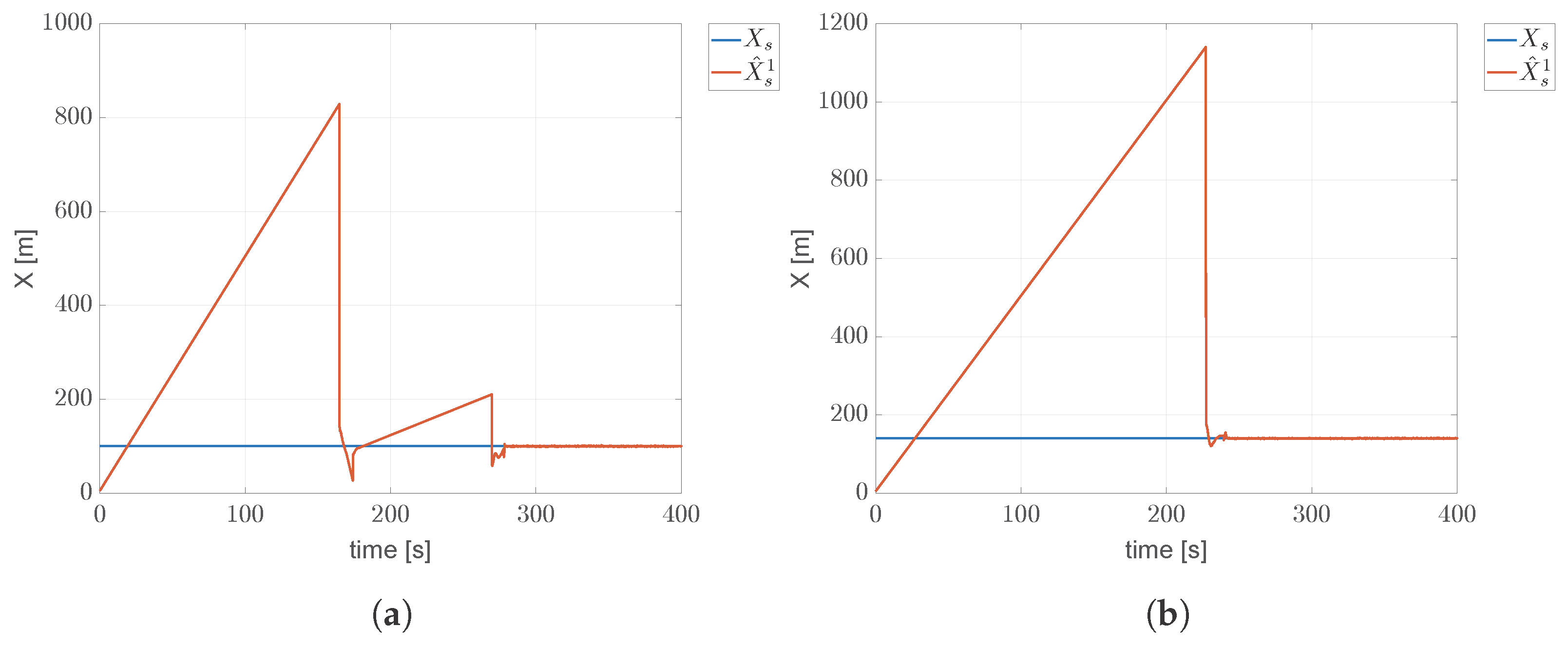
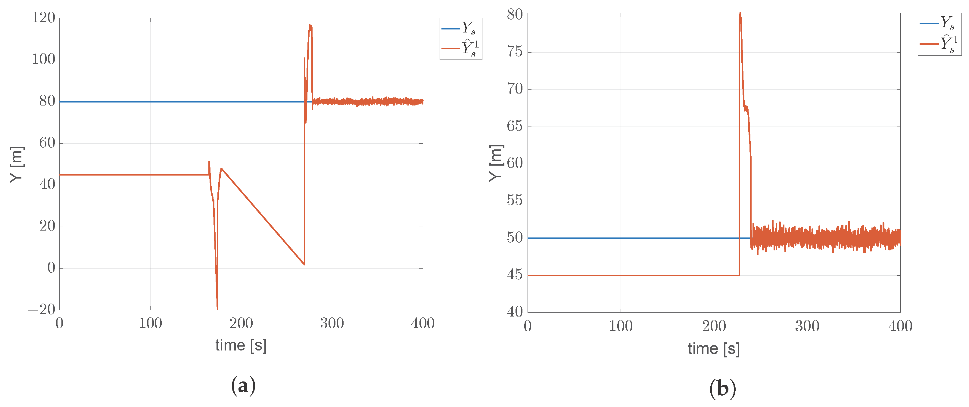
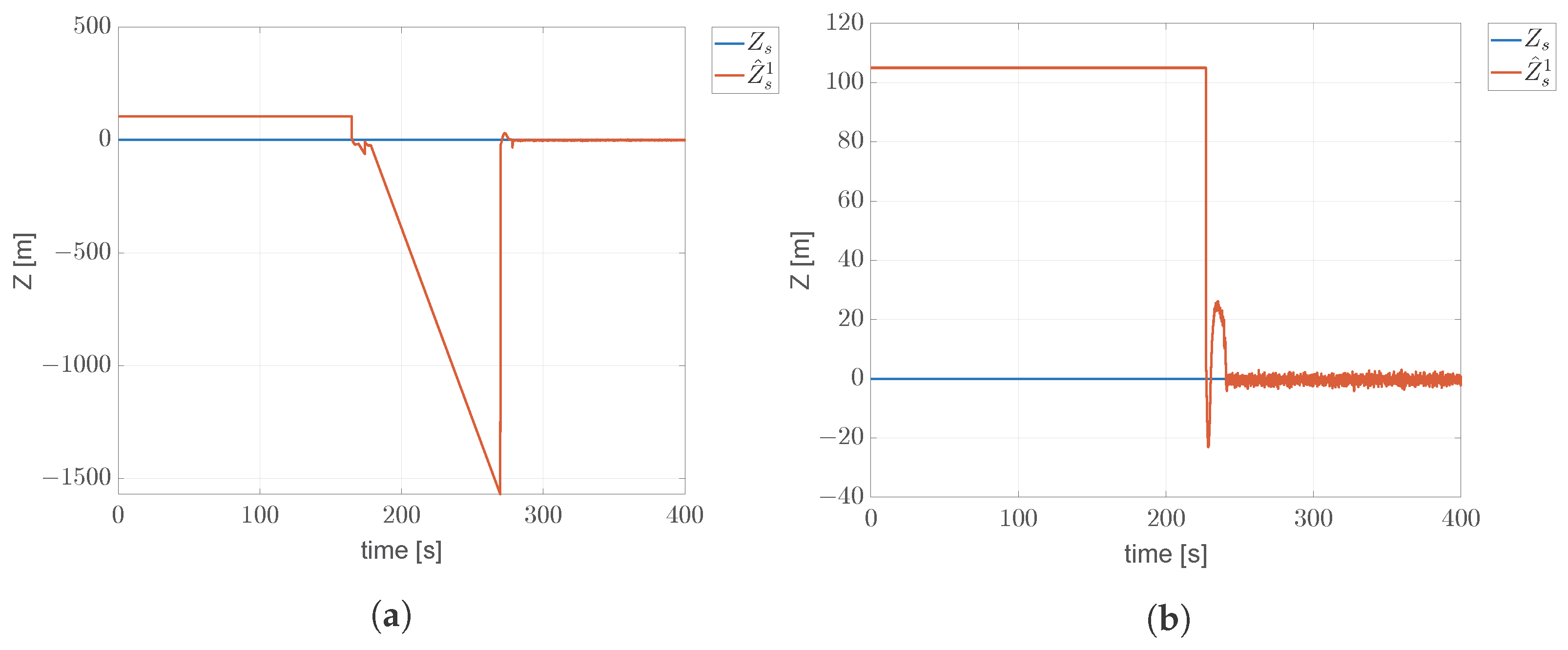
Figure 23, Figure 24 and Figure 25 show the effectiveness of the proposed algorithm in the estimation process of the skier position, comparing the real value with the estimation made by $UA{V}_1$, for both the analyzed case studies. As shown, at the beginning of the simulation the skier position is unknown, still being far from the range of the receivers onboard the UAVs.

Once the skier ARTVA transmitter enters the range of at least three aircraft receivers (at $t=260$ s (#1) and $t=230$ s (#2)), the estimates tend to the real position, converging definitively after the time necessary for the consensus phase.

In case study #1, it is worth noticing that a first convergence estimation is reached at $t=170$ s. This is due to the particular research path; in fact, as shown in Figure 19a, at $t=160$ s the skier enters the sensor range of only one UAV of the swarm, whose measurement is still not sufficient to correctly estimate the position of the missing person (see Section 4.4).

Table 12. Simulation Test #5—Estimation performance in terms of standard deviation and Mean Absolute Error for skier position estimation.

Performance Index	Scenario #1	Scenario #2
${\sigma }_1^{X_t}\left(\mathrm{m}\right)$	0.6498	0.6690
${\sigma }_1^{Y_t}\left(\mathrm{m}\right)$	0.6707	0.6547
${\sigma }_1^{Z_t}\left(\mathrm{m}\right)$	1.1234	1.0879
$MA{E}_1^{X_t}\left(\mathrm{m}\right)$	0.1343	0.0727
$MA{E}_1^{Y_t}\left(\mathrm{m}\right)$	0.0778	0.0331
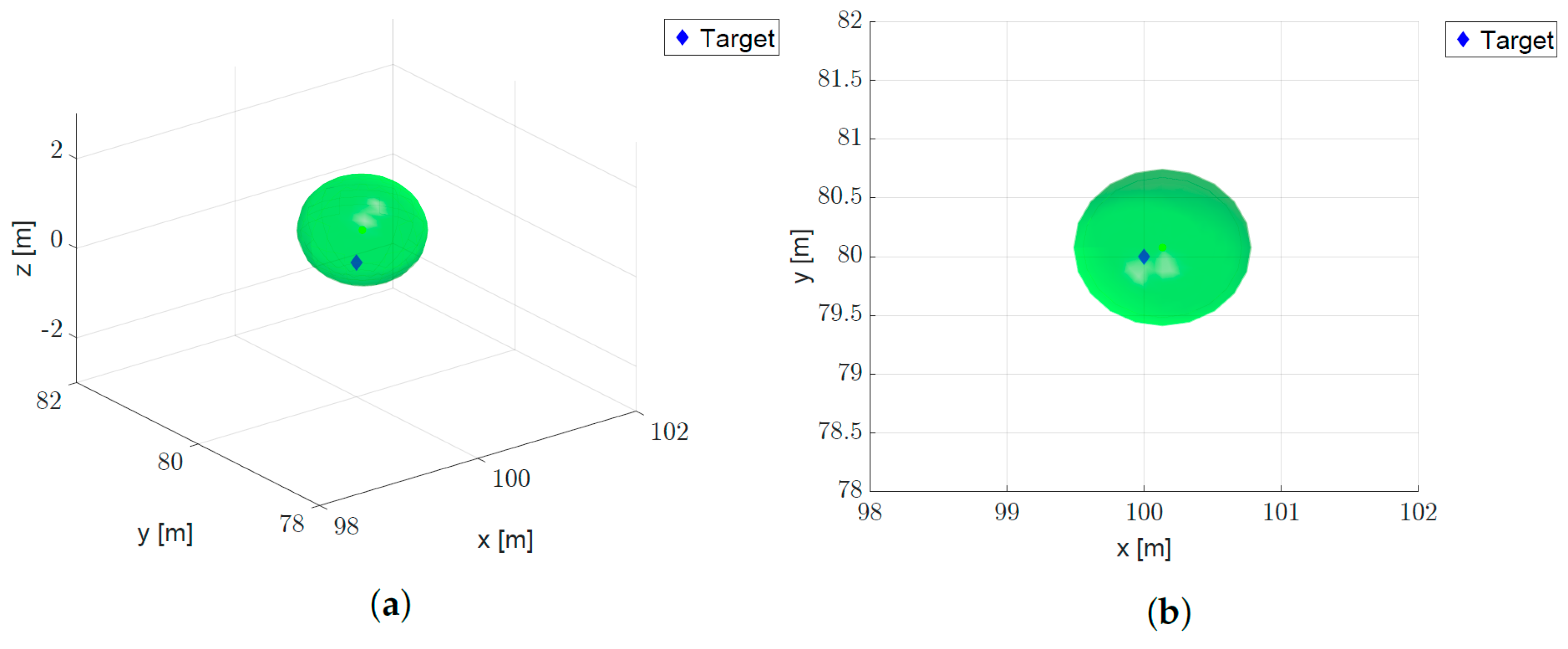
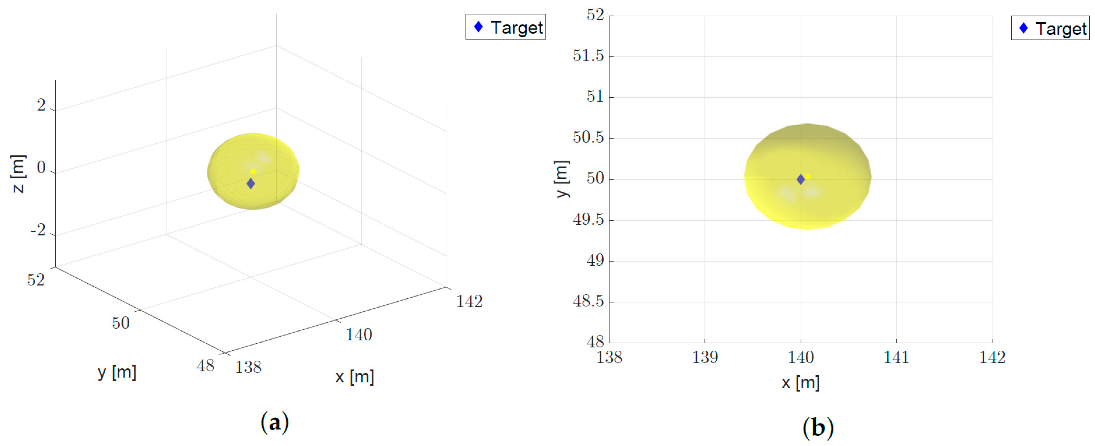
$MA{E}_1^{Z_t}\left(\mathrm{m}\right)$	0.6035	0.3248

shows mean absolute error (Equation (53)) and standard deviation (Equation (54)) for any component of the target position vector, ${\mathit{S}}_s$. These uncertainties in the estimation are graphically represented in Figure 26 and Figure 27 for both the scenarios.

The data presented in this section represent the results regarding the accuracy of the proposed algorithm, with standard deviations never exceeding 1 m and MAE values consistently below 0.1 m for the estimation of the X and Y coordinates. Furthermore, the potential application of the proposed GNC model in SAR scenarios is demonstrated. The aircraft can promptly estimate the position of the missing skier when trilateration is feasible. Additionally, the swarm consistently follows the predetermined search path, using the situational awareness provided by the local estimates.

5. Limitations and Discussion

Several numerical simulations were carried out to highlight the advantages and disadvantages of the proposed procedure in the following contexts: (1) the ability to achieve situational awareness regarding the position and speed of each agent in the formation; (2) the capability to localize a static target in a distributed manner using the transceivers on each UAV; (3) resilience to communication delays and interruptions; and (4) integration with a comprehensive guidance, navigation and control procedure, simulating a realistic post-avalanche search-and-rescue mission.

Regarding the ability to achieve situational awareness, a sensitivity analysis of the main parameters showed that the algorithm is nearly insensitive to the number of communication steps, at least when dealing with a limited number of UAVs. Instead, performance is primarily influenced by the communication scheme. As expected, the topology of the communication graph is crucial, representing how the agents share information among themselves. The communication scheme $\mathcal{A}={\mathcal{A}}_2$ is considered the worst-case scenario and is thus employed in the other tests.

From the perspective of target localization capability, a comparison with a centralized EKF showed that the proposed algorithm achieves nearly identical performance in terms of target localization, as presented in Table 7, for both the $MAE$ and standard deviation $\sigma$. The distributed procedure is only 5 s slower than the centralized one, as depicted in Figure 9, Figure 10 and Figure 11.

The robustness to communication delays and interruptions was confirmed through numerical simulations. These assessments included evaluating the algorithm capability to resume UAV position estimation following disruptions in communication links at specified time intervals (Figure 7) and showing the convergence capabilities in the presence of three different constant communication delays among UAVs (Figure 14). As observed, the position estimation is temporarily interrupted during communication loss but promptly resumes once the connection among agents is re-established. The procedure remains resilient to communication delays, albeit affecting the convergence time for target localization, as expected.

Finally, the last set of simulation results proves the algorithm capability to be employed within a comprehensive guidance navigation and control procedure. It has been demonstrated to be useful in estimating UAV positions, which are essential for trajectory tracking, collision avoidance and target localization. The results show a localization error of less than 1 m, with no faults during the mission.

6. Conclusions

The main objective of this paper was to develop a distributed navigation algorithm for a swarm of UAVs to estimate the position of a target in the operational scenario. The aim of the algorithm is to provide situational awareness to the aircraft formation and eliminate the need for a central unit, thereby making it scalable and computationally efficient.

The proposed algorithm combined the advantages of the hybrid consensus on measurements and consensus on information (HCMCI) technique with the internodal transformation theory (ITT). This combination allowed for the distributed estimation of the swarm overall state and the detection of the target position. The algorithm was designed to be adaptable to various swarm architectures and environments, enabling the swarm to self-organize and adjust its configuration over time.

Numerical analyses were conducted to evaluate the algorithm effectiveness. A sensitivity analysis was performed to assess its performance by varying the main operational parameters and communication link schemes.

Results highlight that performance is not significantly improved by increasing the number of consensus steps which, on the other hand, increases the time required to execute the consensus algorithm. Furthermore, as expected, the graph topology can improve algorithm convergence by optimizing communication.

Regarding reliability, it is observed that communication delays can decrease the convergence capability, as intuitively expected. However, in realistic scenarios with small delays (approximately $0.1$ s), it does not adversely affect performance.

Furthermore, some simulation tests were also conducted to evaluate the algorithm’s ability to resume estimation after communication interruptions and to estimate the position of a fixed target. A comparison with a centralized version of the EKF was included to evaluate the performance trade-offs of the decentralized technique.

The proposed navigation algorithm successfully achieved the objectives outlined in this paper, demonstrating its capability to estimate the target position and maintain overall situational awareness.

Future research in this field should explore the possibility of detecting and isolating multiple targets, which would represent another important factor in enhancing the effectiveness of such algorithms in emergency scenarios.