

Computational Model for Tree-like Fractals Used as Internal Structures for Additive Manufacturing Parts


Abstract
:1. Introduction
2. Modelling Tree-like Fractal Structures into CAD Parts
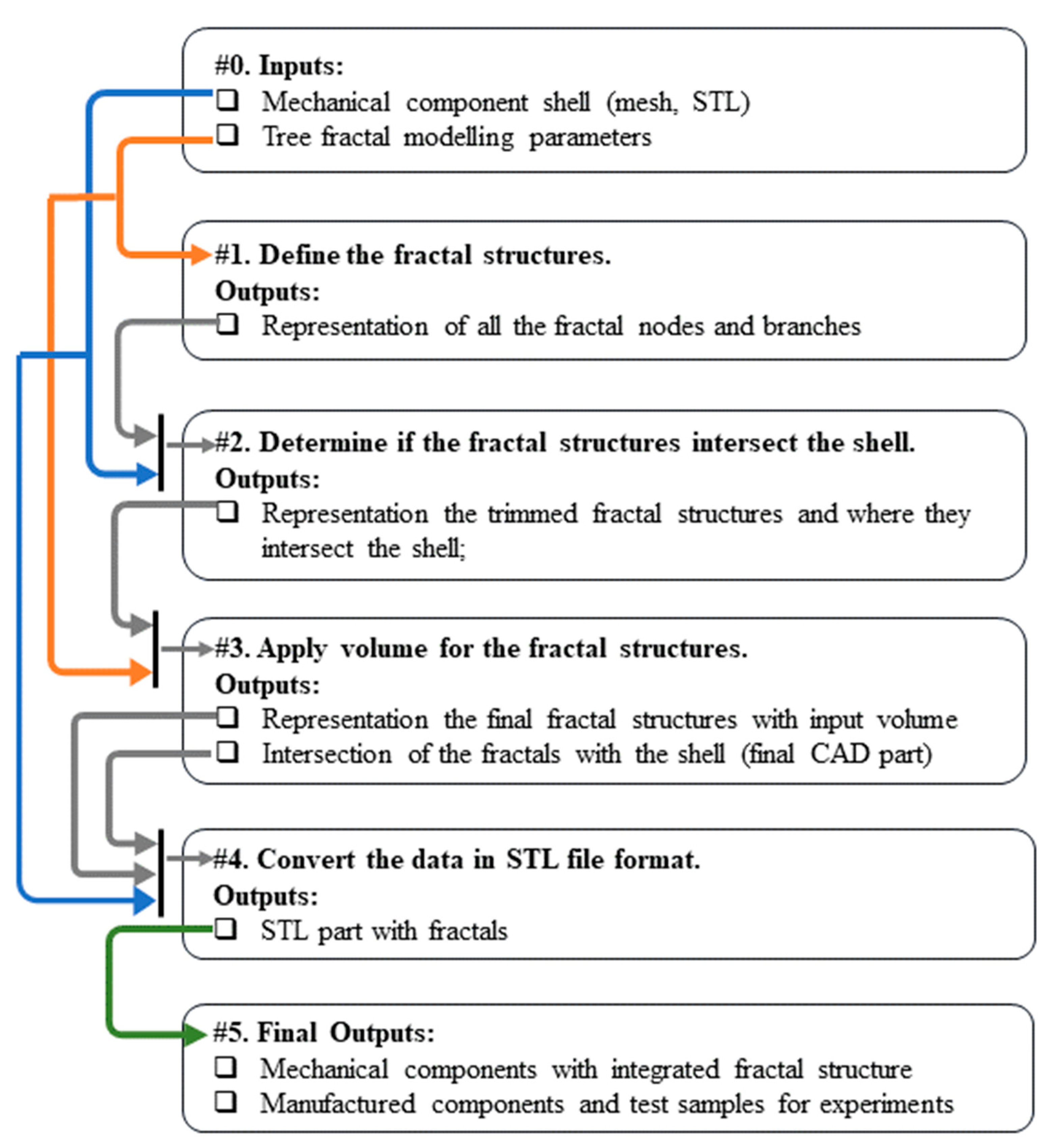
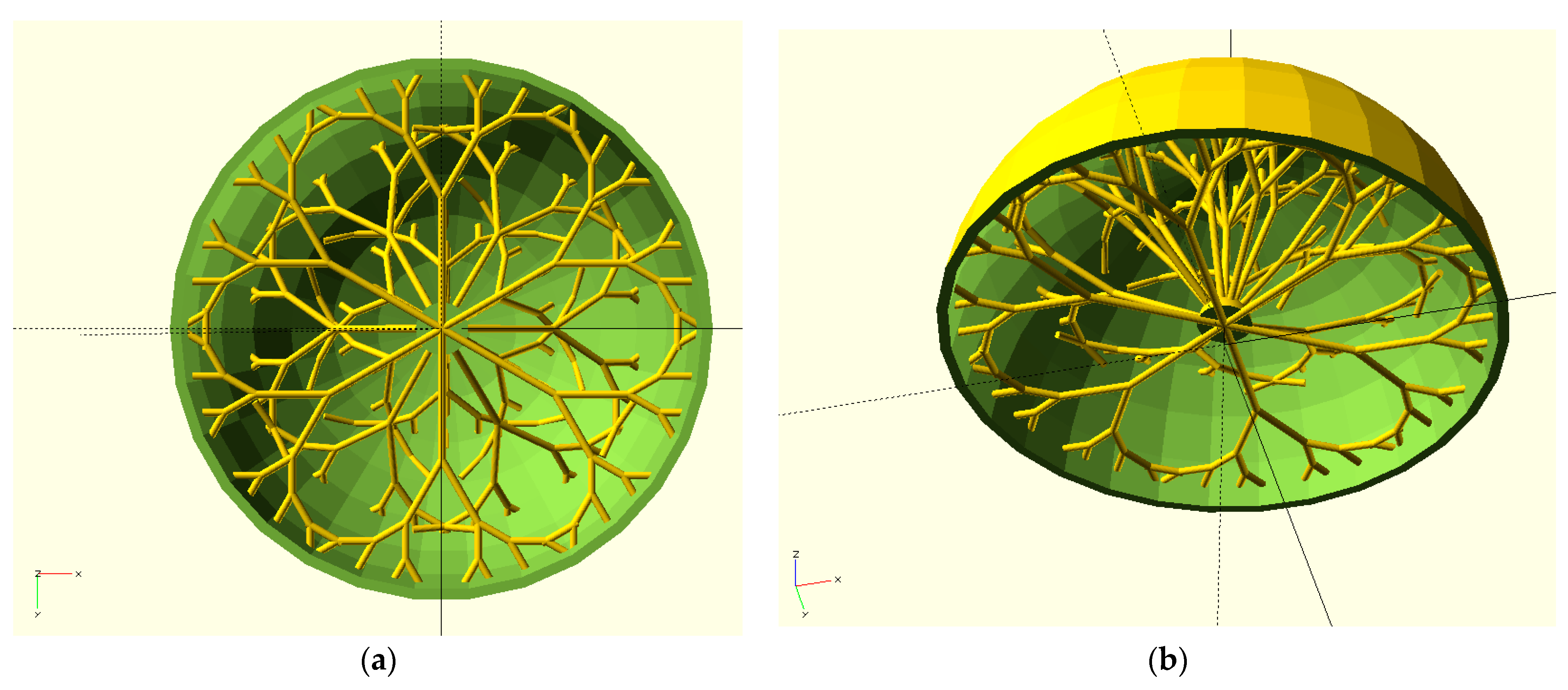
- Step #0 defines the inputs for the algorithm. The first input is the CAD shell, expressed as a CAD model with internal cavities that require fractal filling. Figure 2 shows an example of a CAD shell formed by two hemispheres. Note that the shell is not necessarily a continuous solid as long as the discontinuous volume is filled with fractal structures, such as in instances where the fractals connect the multiple parts into a single rigid body. The algorithm’s second input is a fractal parameter list (roots, branches, angles, etc.) detailed in Section 3.
- Step #1 computes a complete representation of the fractal structure based on the input parameters. This representation is one-dimensional, meaning that the fractal is defined only using points and line segments at this stage.
- Step #2 computes the intersection of each fractal structure (computed in Step#1) with the CAD shell. The goal is to connect the fractals with the shell without any artifacts remaining on the outer surface of the part. The output of this step is a fractal representation where branches that intersect the shell are trimmed. This representation is also one-dimensional.
- Step #3 applies volume to the one-dimensional fractal structures (the trimmed representation from Step#2). In this step, each fractal branch (represented by a line segment) is converted into a cylinder (radius provided in the inputs from Step#0), and all the cylinders form a union (the physical fractal structures). Furthermore, the physical fractal structures are united with the shell, resulting in the final CAD part.
- Step #4 converts the CAD part (fractal structures united with the shell) into an STL file format for manufacturing or FEA.
- Step #5 represents the final outputs of the algorithm. On the one hand, we can manufacture lightweight parts for various applications or testing samples. On the other hand, the CAD data are provided for FEA.
3. Mathematical Modeling of Tree-like Fractals
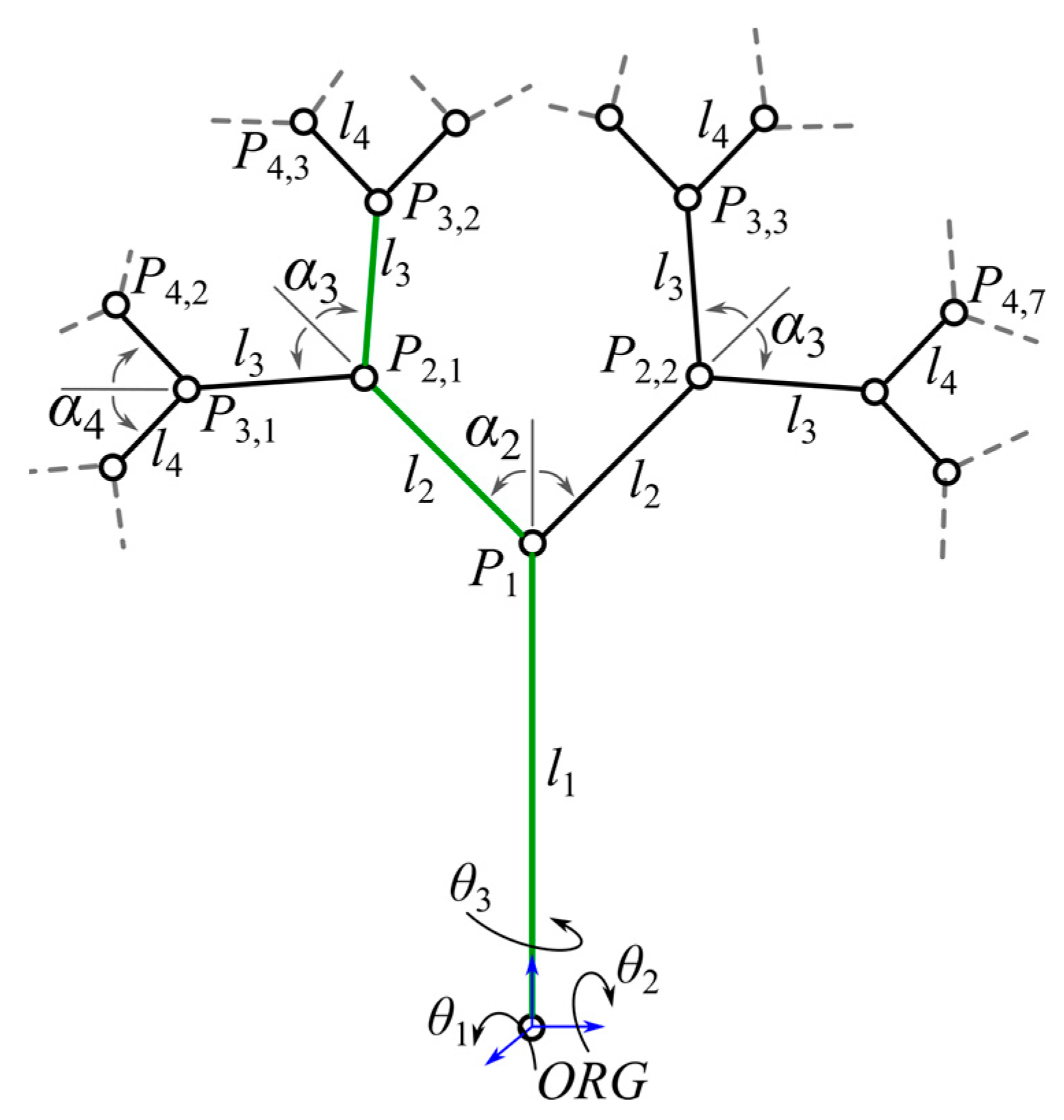
- The points Pi,j represent the nodes of the fractal.
- A branch is represented by a line segment of length li connecting two nodes.
- A node Pi, is a child node of Pk, if: (1) i > k; and (2) the branches of lengths lm that connect the two nodes always respect m > k. For example, P3,1 is a child of P2,1, whereas P3,3 is not (Figure 3).
- A node Pi is a parent node if it has at least one child node.
- A leaf is the final node.
- ORG represents the origin (root) of the fractal. The root is displaced (linearly) from a global coordinate system OXYZ by a vector [VX, VY, VZ]T. Furthermore, the orientation of the first branch is given by the angles θ1, θ2, θ3 (using a ZYX rotation convention).
- αi are angles between two connected branches.
- Subtracting each (i − 1) from i rows i > 1,
- Removing the redundancies (multiple points repeating) in the table,
| Algorithm 1: Table representation for tree-like fractals. |
|
4. Computational Model for Surface-Fractal Intersections
- A surface mesh with a given set of points denoted PTS and triangulation denoted TR.
- A tabular fractal representation.
| Algorithm 2: Table representation for trimmed tree-like fractals. |
compute intersection point IP if IP exists: break end for
|
5. Applying Volume to the Fractal Structures
- Geometric computational method (suitable when the shell is defined by a surface shell but not for CAD format). In this approach, the cylinders are defined by 3D Cartesian points used to compute surface meshes. The surface meshes are stitched to obtain the final structure, which is stitched to the CAD shell.
- CAD method (suitable in both cases). If the shell is defined by a surface mesh with triangulations, the mesh is converted first in CAD format. The fractal cylinders are generated and united with the CAD shell using CAD software.
5.1. The Geometric Computational Method
- Stitch three branches at a node; to apply volume, branches are defined as cylinders with given height, orientation, and radii. The process of stitching branches at a node computes the union of three cylinders, and it is useful to generate fractal structures.
- Stitch one branch to a given surface mesh; the branches that do not intersect through nodes are stitched to the shell. This process enables the computation of the final surface mesh (the desired part).
- st1.1.
- Three cylinders are defined with heights constructed using Equation (14); CYL1 (defining the main/parent branch) with height defined by starting point Pi1 and endpoint Pf1; CYL2 (defining the first secondary/child branch) with starting point Pi2 and endpoint Pf2; and CYL3 (defining the second secondary/child branch) with starting point Pi3 and endpoint Pf3 (cells within tables such as, e.g., Table 5, contain information for all of the fractal branches).
- st1.2.
- All cylinders are created such that they contain a set of generators (straight lines on the surface of the cylinder), each generator with a known number of points; the set G1 is defined for CYL1 with g1i ∈ G1 (i = 1…n1), and each generator contains points p1ij ∈ g1i (j = 1…m1); furthermore, G2 is defined for CYL2 with g2i ∈ G2 (i = 1…m2), with the points p2ij ∈ g2i (j = 1…m2); finally G3 is defined for CYL3 with g3i ∈ G3 (i = 1…m3), and p3ij ∈ g3i (j = 1…m3). The n’s denote the number of generators of each cylinder, whereas the m’s denote the number of points of each generator. Figure 5 shows an example of three cylinders: (1) the first cylinder with Pi1 = [0 0 0] [mm], Pf1 = [0 0 15] [mm], radius R1 = 4 [mm], n1 = 80, m1 = 80; the second cylinder with Pi2 = [0 0 15] [mm], Pf2 = [0 5 25] [mm], radius R2 = 4 [mm], n2 = 80, m2 = 80; and the third cylinder with Pi3 = [0 0 15] [mm], Pf3 = [0 –5 25] [mm], radius R3 = 4 [mm], n3 = 80, m3 = 80. For each cylinder, the first three generators (g11, g12, and g13 from G1; g21, g22, and g23 from G2; and g31, g32, and g33 from G3) are colored differently to highlight the cylinder construction rules.
- st1.3.
- Three vectors are defined (using Equation (15)): V1 normal to the plane that contains the final circle face of the first cylinder (centered at Pf1); V2 normal to the plane that contains the first circle face (base) of the second cylinder (centered at Pi2); V3 normal to the plane that contains the first circle face (base) of the third cylinder (centered at Pi3). Three bisector vectors are defined using Equation (16).
- st1.4.
- Three cutoff planes (i.e., the planes that trim the cylinders such that the intersecting volumes are discarded) Δ1, Δ2, Δ3 are defined, with the normal vectors being the bisector vectors within Equation (16), and all three planes pass through Pf1:
- st1.5.
- To trim CYL1 with the Δ1 and Δ2 planes, the points p1ij of the generators g1i form the set G1 substituted in the x, y, z parameters of Equations (19a) and (19b) and must respect the inequalities Δ1 < 0, Δ2 < 0. To trim CYL2 with Δ1 and Δ3 planes, the points p2ij of the generators g2i form the set G3 (after substitution in Equations (19a) and (19b)) and must respect the inequalities Δ1 > 0, Δ3 > 0. Finally, to trim CYL3 with Δ2 and Δ3 planes, the points p3ij of the generators g3i form the set G3 (after substitution in Equations (19b) and (19c)) and must respect the inequalities Δ2 > 0, Δ3 > 0.
- st1.6.
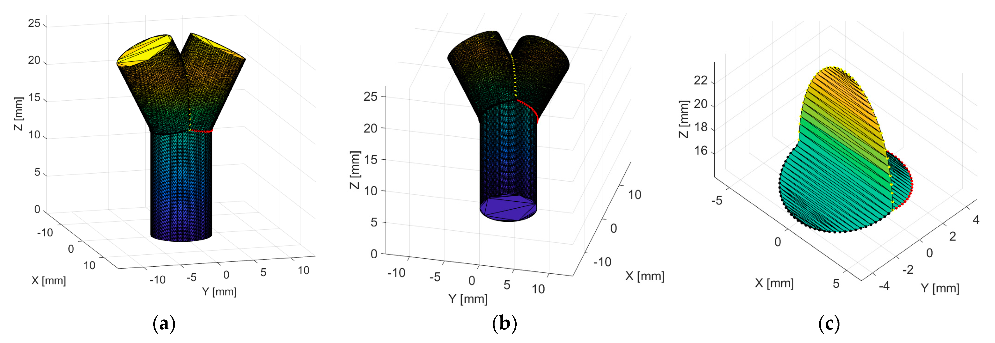
- The last points (for all of the generators for all of the cylinders) that respect the inequalities defined in the previous step are projected in the cutoff planes to define the edge curves (denoted γ) of the cylinders’ intersection. The following sequential algorithm is used (presented in general form):
- st1.7.
- An alpha shape is computed (in Matlab, the function is alphaShape [20]) for each of the three trimmed cylinders (with the added edges), and the boundary facets [21] are selected; this yields surface meshes with 3D points and their corresponding triangulation. For the union of the three cylinders, the 3D points of the three trimmed cylinders are concatenated. The triangulations are also concatenated after the necessary change in the indexing of the triangle vertices, e.g., if the first cylinder has 101 points, each triangle vertex of the second cylinder must add 101 and so on (to avoid overlapping triangulations). Moreover, the triangles containing only vertices from the intersection edge γ are discarded (to ensure correct surface stitching). Figure 7 shows the union of three cylinders (previously illustrated in Figure 5).
- st2.1.
- A surface mesh α is given with a set of Cartesian points ki ∈ K (i = 1…n*) (n* being the total number of points) and a set of triangulations tj ∈ T (j = 1…m*) (m* being the number of triangles with vertices ∈ K). Furthermore, a cylinder CYL is defined with height by starting point Pi and endpoint Pf. The cylinder is constructed (again) using a set of generators, and each generator has a distinct set of points; the set G is defined for CYL with gi ∈ G (i = 1…n), and each generator contains points pij ∈ g1i (j = 1…m). The direction vector of the cylinders’ heights and generators is given by Equation (13).
- st2.2.
- All generators gi ∈ G are tested for intersection with the mesh α using the ray/triangle intersection algorithm (Möller and Trumbore) [19] for every triangle in T. To achieve this, a vector V is defined using the first and last points of the generator, and if the generator intersects a triangle tj ∈ T, the quantity norm(V) is compared with the distance D from the ray origin to the intersection point. If norm(V) ≥ D, the intersection point is considered a point on the intersection edge γ. Only geometric configurations that produce an intersection point for every gi ∈ G are allowed (the CAD method is used if this is not true).
- st2.3.
- The cylinder CYL is trimmed. The points pij ∈ gi up to the intersection point (on the edge γ) are kept, and the points of the edge γ are concatenated, resulting in a set G’1.
- st2.4.
- The shape α is trimmed. The points ki ∈ K that are inside the CYL (before trimming) are discarded, and the points of the edge γ are concatenated, resulting in a set k’i ∈ K’.
- st2.5.
- Two alpha shapes are computed, α1 for K’ and α2 for G’1. Then, boundary facets are computed for α1 containing the Cartesian points k’i ∈ K’ (i = 1…n’) and a new triangulation with t’j ∈ T’ (j = 1…m’), and for α2 containing the Cartesian points p’ij ∈ G’ (j = 1…n’’) and a triangulation t’’j ∈ T’’ (j = 1…m’’).
- st2.6.
- The triangles t’j ∈ T’ and t’’j ∈ T’’ that have all three vertices point from the intersection edge γ are discarded. Furthermore, the final surface mesh αfinal is defined with the Cartesian points kfinal,i ∈ K’ ∪ G’1 (i = 1… n’+ n’’) and the triangulation tfinal,j ∈ T’ ∪ T’’ (j = 1… m’+ m’’) where T’’ = T’’ + max(T’) (to account for the triangulation concatenation).
| Algorithm 3: CAD part with fractals (geometric method). |
end for
|
5.2. The CAD Method
- st3.1.
- A SCAD structure is initialized as the workspace, and the CAD shell is imported.
- st3.2.
- The length Hi,j of each branch B of the fractal structure (data arranged in tables such as, e.g., Table 4 or Table 5) is computed using Equation (16). The initial point Pinit of each branch is also found in the fractal data. If a surface mesh is provided, the following must be considered:
- a.
- For thin shells (thickness in the order of the radii of the cylinders composing the fractals), even if the fractals are trimmed due to surface intersection, trimming with a CAD tool is recommended (see step st3.5).
- b.
- For thick shells (thickness in the order of at least two times the cylinder radii), no CAD tool trimming is required.
- st3.3.
- For each branch, a cylinder CYLi,j is created in CAD with height Hi,j, and radius R (given in Step#0).
- st3.4.
- Each cylinder CYLi,j is generated at the origin of the world coordinate system. Therefore, to position the branch correctly, each cylinder is rotated using the angles ψ and φ (Equation (17)) and then translated using Pinit. The cylinder is then united with the rest of the CAD structures (other cylinders within the fractals and the shell).
- st3.5.
- A CAD trimming tool, which is the negative of the shell, is used on every generated cylinder (assuming it is needed).
| Algorithm 4: CAD part with fractals (CAD method). |
else if the CAD shell is thick, then goto 5 if the fractal structures are not trimmed (e.g., Table 4), then goto 4
end for
end for
|
6. Case Studies
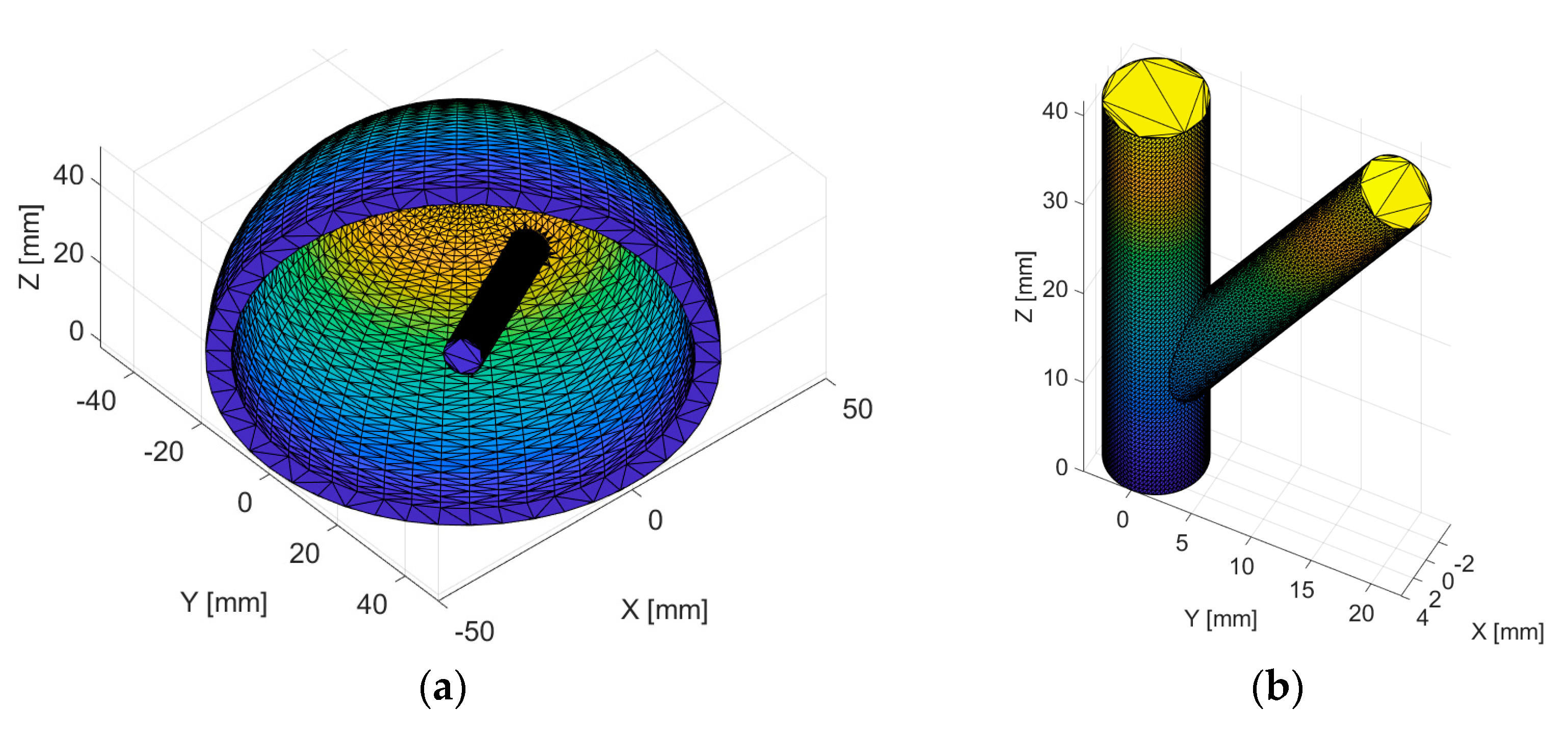
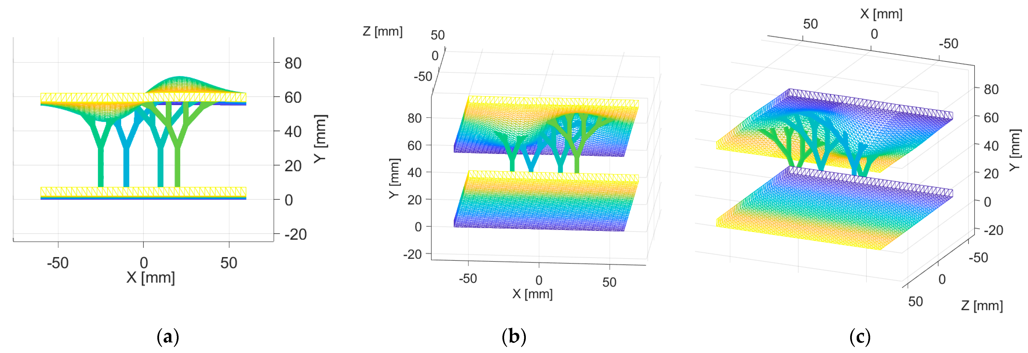
6.1. Creating Fractal Structures on a Surface Mesh Using the Geometric Method
6.2. Creating Fractal Structures on a Hemispherical Shell Using the CAD Method
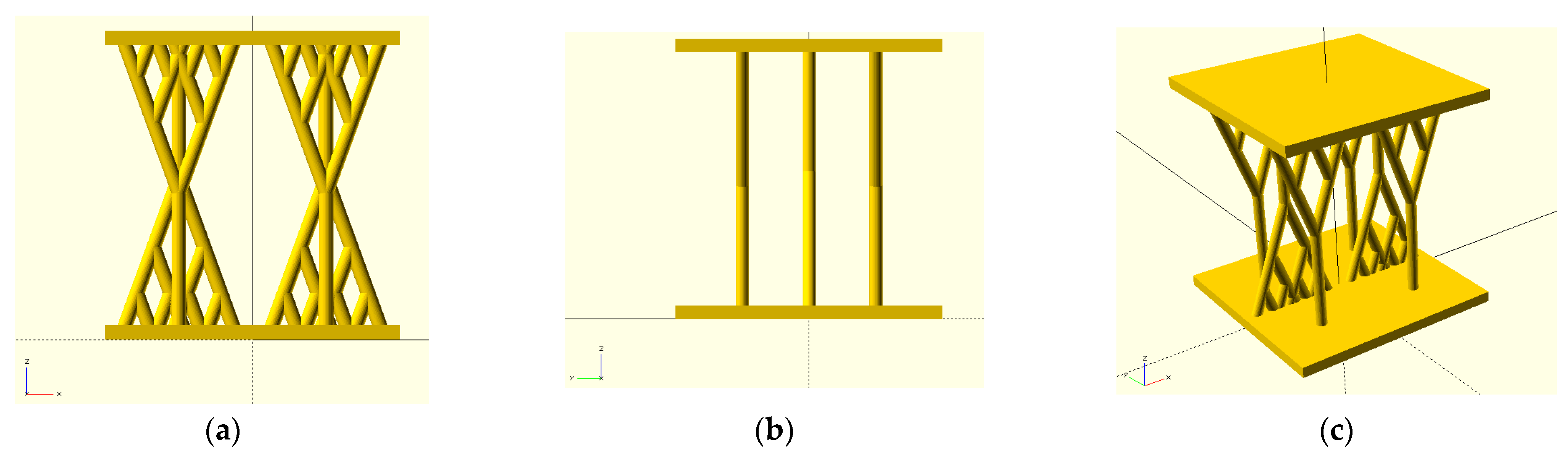
6.3. Creating Test Samples with Fractal Structures Using the CAD Method
7. Conclusions
Author Contributions
Funding
Conflicts of Interest
Appendix A

| α1 = 0, l1 = 28 | α = 0, l1 = 28 | α1 = 0, l1 = 28 | α1 = 0, l1 = 28 | α1 = 0, l1 = 28 | α1 = 0, l1 = 28 | α1 = 0, l1 = 28 | α1 = 0, l1 = 28 | α1 = 0, l1 = 28 | α =0, l1 = 28 | α1 = 0, l1 = 28 | α1 = 0, l1 = 28 | α1 = 0, l1 = 28 | α1 = 0, l1 = 28 | α1 = 0, l1 = 28 | α1 = 0, l1 = 28 |
| α2 = π/9, l2 = 14 | α2 = π/9, l2 = 14 | α2 = π/9, l2 = 14 | α2 = π/9, l2 = 14 | α2 = π/9, l2 = 14 | α2 = π/9, l2 = 14 | α2 = π/9, l2 = 14 | α2 = π/9, l2 = 14 | α2 = −π/9, l2 = 14 | α2 = −π/9, l2 = 14 | α2 = −π/9, l2 = 14 | α2 = −π/9, l2 = 14 | α2 = −π/9, l2 = 14 | α2 = −π/9, l2 = 14 | α2 = −π/9, l2 = 14 | α2 = −π/9, l2 = 14 |
| α3 = π/9, l3 = 14 | α3 = π/9, l3 = 14 | α3 = π/9, l3 = 14 | α3 = π/9, l3 = 14 | α3 = −π/9, l3 = 14 | α3 = −π/9, l3 = 14 | α3 = −π/9, l3 = 14 | α3 = −π/9, l3 = 14 | α3 = π/9, l3 = 14 | α3 = π/9, l3 = 14 | α3 = π/9, l3 = 14 | α3 = π/9, l3 = 14 | α3 = −π/9, l3 = 14 | α3 = −π/9, l3 = 14 | α3 = −π/9, l3 = 14 | α3 = −π/9, l3 = 14 |
| α4 = π/9, l4 = 14 | α4 = π/9, l4 = 14 | α4 = −π/9, l4 = 14 | α4 = −π/9, l4 = 14 | α4 = π/9, l4 = 14 | α4 = π/9, l4 = 14 | α4 = −π/9, l4 = 14 | α4 = −π/9, l4 = 14 | α4 = π/9, l4 = 14 | α4 = π/9, l4 = 14 | α4 = −π/9, l4 = 14 | α4 = −π/9, l4 = 14 | α4 = π/9, l4 = 14 | α4 = π/9, l4 = 14 | α4 = −π/9, l4 = 14 | α4 = −π/9, l4 = 14 |
| α5 = π/9, l5 = 14 | α5 = −π/9, l5 = 14 | α5 = π/9, l5 = 14 | α5 = −π/9, l5 = 14 | α5 = π/9, l5 = 14 | α5 = −π/9, l5 = 14 | α5 = π/9, l5 = 14 | α5 = −π/9, l5 = 14 | α5 = π/9, l5 = 14 | α5 = −π/9, l5 = 14 | α5 = π/9, l5 = 14 | α5 = −π/9, l5 = 14 | α5 = π/9, l5 = 14 | α5 = −π/9, l5 = 14 | α5 = π/9, l5 = 14 | α5 = −π/9, l5 = 14 |
| α1 = 0, l1 = 28 | α = 0, l1 = 28 | α1 = 0, l1 = 28 | α1 = 0, l1 = 28 | α1 = 0, l1 = 28 | α1 = 0, l1 = 28 | α1 = 0, l1 = 28 | α1 = 0, l1 = 28 | α1 = 0, l1 = 28 | α =0, l1 = 28 | α1 = 0, l1 = 28 | α1 = 0, l1 = 28 | α1 = 0, l1 = 28 | α1 = 0, l1 = 28 | α1 = 0, l1 = 28 | α1 = 0, l1 = 28 |
| α2 = π/8, l2 = 14 | α2 = π/8, l2 = 14 | α2 = π/8, l2 = 14 | α2 = π/8, l2 = 14 | α2 = π/8, l2 = 14 | α2 = π/8, l2 = 14 | α2 = π/8, l2 = 14 | α2 = π/8, l2 = 14 | α2 = −π/9, l2 = 14 | α2 = −π/9, l2 = 14 | α2 = −π/9, l2 = 14 | α2 = −π/9, l2 = 14 | α2 = −π/9, l2 = 14 | α2 = −π/9, l2 = 14 | α2 = −π/9, l2 = 14 | α2 = −π/9, l2 = 14 |
| α3 = π/9, l3 = 14 | α3 = π/9, l3 = 14 | α3 = π/9, l3 = 14 | α3 = π/9, l3 = 14 | α3 = −π/8, l3 = 14 | α3 = −π/8, l3 = 14 | α3 = −π/8, l3 = 14 | α3 = −π/8, l3 = 14 | α3 = π/9, l3 = 14 | α3 = π/9, l3 = 14 | α3 = π/9, l3 = 14 | α3 = π/9, l3 = 14 | α3 = −π/8, l3 = 14 | α3 = −π/8, l3 = 14 | α3 = −π/8, l3 = 14 | α3 = −π/8, l3 = 14 |
| α4 = π/8, l4 = 14 | α4 = π/8, l4 = 14 | α4 = −π/9, l4 = 14 | α4 = −π/9, l4 = 14 | α4 = π/8, l4 = 14 | α4 = π/8, l4 = 14 | α4 = −π/9, l4 = 14 | α4 = −π/9, l4 = 14 | α4 = π/8, l4 = 14 | α4 = π/8, l4 = 14 | α4 = −π/9, l4 = 14 | α4 = −π/9, l4 = 14 | α4 = π/8, l4 = 14 | α4 = π/8, l4 = 14 | α4 = −π/9, l4 = 14 | α4 = −π/9, l4 = 14 |
| α5 = π/9, l5 = 14 | α5 = −π/8, l5 = 14 | α5 = π/9, l5 = 14 | α5 = −π/8, l5 = 14 | α5 = π/9, l5 = 14 | α5 = −π/8, l5 = 14 | α5 = π/9, l5 = 14 | α5 = −π/8, l5 = 14 | α5 = π/9, l5 = 14 | α5 = −π/8, l5 = 14 | α5 = π/9, l5 = 14 | α5 = −π/8, l5 = 14 | α5 = π/9, l5 = 14 | α5 = −π/8, l5 = 14 | α5 = π/9, l5 = 14 | α5 = −π/8, l5 = 14 |
| α1 = 0, l1 = 28 | α = 0, l1 = 28 | α1 = 0, l1 = 28 | α1 = 0, l1 = 28 | α1 = 0, l1 = 28 | α1 = 0, l1 = 28 | α1 = 0, l1 = 28 | α1 = 0, l1 = 28 | α1 = 0, l1 = 28 | α = 0, l1 = 28 | α1 = 0, l1 = 28 | α1 = 0, l1 = 28 | α1 = 0, l1 = 28 | α1 = 0, l1 = 28 | α1 = 0, l1 = 28 | α1 = 0, l1 = 28 |
| α2 = π/9, l2 = 14 | α2 = π/9, l2 = 14 | α2 = π/9, l2 = 14 | α2 = π/9, l2 = 14 | α2 = π/9, l2 = 14 | α2 = π/9, l2 = 14 | α2 = π/9, l2 = 14 | α2 = π/9, l2 = 14 | α2 = −π/9, l2 = 14 | α2 = −π/9, l2 = 14 | α2 = −π/9, l2 = 14 | α2 = −π/9, l2 = 14 | α2 = −π/9, l2 = 14 | α2 = −π/9, l2 = 14 | α2 = −π/9, l2 = 14 | α2 = −π/9, l2 = 14 |
| α3 = π/9, l3 = 14 | α3 = π/9, l3 = 14 | α3 = π/9, l3 = 14 | α3 = π/9, l3 = 14 | α3 = −π/9, l3 = 14 | α3 = −π/9, l3 = 14 | α3 = −π/9, l3 = 14 | α3 = −π/9, l3 = 14 | α3 = π/9, l3 = 14 | α3 = π/9, l3 = 14 | α3 = π/9, l3 = 14 | α3 = π/9, l3 = 14 | α3 = −π/9, l3 = 14 | α3 = −π/9, l3 = 14 | α3 = −π/9, l3 = 14 | α3 = −π/9, l3 = 14 |
| α4 = π/9, l4 = 14 | α4 = π/9, l4 = 14 | α4 = −π/9, l4 = 14 | α4 = −π/9, l4 = 14 | α4 = π/9, l4 = 14 | α4 = π/9, l4 = 14 | α4 = −π/9, l4 = 14 | α4 = −π/9, l4 = 14 | α4 = π/9, l4 = 14 | α4 = π/9, l4 = 14 | α4 = −π/9, l4 = 14 | α4 = −π/9, l4 = 14 | α4 = π/9, l4 = 14 | α4 = π/9, l4 = 14 | α4 = −π/9, l4 = 14 | α4 = −π/9, l4 = 14 |
| α5 = π/9, l5 = 14 | α5 = −π/9, l5 = 14 | α5 = π/9, l5 = 14 | α5 = −π/9, l5 = 14 | α5 = π/9, l5 = 14 | α5 = −π/9, l5 = 14 | α5 = π/9, l5 = 14 | α5 = −π/9, l5 = 14 | α5 = π/9, l5 = 14 | α5 = −π/9, l5 = 14 | α5 = π/9, l5 = 14 | α5 = −π/9, l5 = 14 | α5 = π/9, l5 = 14 | α5 = −π/9, l5 = 14 | α5 = π/9, l5 = 14 | α5 = −π/9, l5 = 14 |
| α1 = 0, l1 = 28 | α = 0, l1 = 28 | α1 = 0, l1 = 28 | α1 = 0, l1 = 28 | α1 = 0, l1 = 28 | α1 = 0, l1 = 28 | α1 = 0, l1 = 28 | α1 = 0, l1 = 28 | α1 = 0, l1 = 28 | α = 0, l1 = 28 | α1 = 0, l1 = 28 | α1 = 0, l1 = 28 | α1 = 0, l1 = 28 | α1 = 0, l1 = 28 | α1 = 0, l1 = 28 | α1 = 0, l1 = 28 |
| α2 = π/9, l2 = 14 | α2 = π/9, l2 = 14 | α2 = π/9, l2 = 14 | α2 = π/9, l2 = 14 | α2 = π/9, l2 = 14 | α2 = π/9, l2 = 14 | α2 = π/9, l2 = 14 | α2 = π/9, l2 = 14 | α2 = −π/8, l2 = 16 | α2 = −π/8, l2 = 16 | α2 = −π/8, l2 = 16 | α2 = −π/8, l2 = 16 | α2 = −π/8, l2 = 16 | α2 = −π/8, l2 = 16 | α2 = −π/8, l2 = 16 | α2 = −π/8, l2 = 16 |
| α3 = π/9, l3 = 14 | α3 = π/9, l3 = 14 | α3 = π/9, l3 = 14 | α3 = π/9, l3 = 14 | α3 = −π/9, l3 = 16 | α3 = −π/9, l3 = 16 | α3 = −π/9, l3 = 16 | α3 = −π/9, l3 = 16 | α3 = π/9, l3 = 14 | α3 = π/9, l3 = 14 | α3 = π/9, l3 = 14 | α3 = π/9, l3 = 14 | α3 = −π/9, l3 = 16 | α3 = −π/9, l3 = 16 | α3 = −π/9, l3 = 16 | α3 = −π/9, l3 = 16 |
| α4 = π/9, l4 = 14 | α4 = π/9, l4 = 14 | α4 = −π/8, l4 = 16 | α4 = −π/8, l4 = 16 | α4 = π/9, l4 = 14 | α4 = π/9, l4 = 14 | α4 = −π/8, l4 = 16 | α4 = −π/8, l4 = 16 | α4 = π/9, l4 = 14 | α4 = π/9, l4 = 14 | α4 = −π/8, l4 = 16 | α4 = −π/8, l4 = 16 | α4 = π/9, l4 = 14 | α4 = π/9, l4 = 14 | α4 = −π/8, l4 = 16 | α4 = −π/8, l4 = 16 |
| α5 = π/9, l5 = 14 | α5 = −π/9, l5 = 16 | α5 = π/9, l5 = 14 | α5 = −π/9, l5 = 16 | α5 = π/9, l5 = 14 | α5 = −π/9, l5 = 16 | α5 = π/9, l5 = 14 | α5 = −π/9, l5 = 16 | α5 = π/9, l5 = 14 | α5 = −π/9, l5 = 16 | α5 = π/9, l5 = 14 | α5 = −π/9, l5 = 16 | α5 = π/9, l5 = 14 | α5 = −π/9, l5 = 16 | α5 = π/9, l5 = 14 | α5 = −π/9, l5 = 16 |
| [10, 1, 0] | NaN | NaN | NaN | NaN | NaN | NaN | NaN | NaN | NaN | NaN | NaN | NaN | NaN | NaN | NaN |
| [10, 29, 0] — [10, 1, 0] | NaN | NaN | NaN | NaN | NaN | NaN | NaN | NaN | NaN | NaN | NaN | NaN | NaN | NaN | NaN |
| [5.2, 42.2, 0] — [10, 29, 0] | [14.8, 42.2, 0] — [10, 29, 0] | NaN | NaN | NaN | NaN | NaN | NaN | NaN | NaN | NaN | NaN | NaN | NaN | NaN | NaN |
| [−3.8, 52.9, 0] — [5.2, 42.2, 0] | [5.2, 56.2, 0] — [5.2, 42.2, 0] | [14.8, 56.2, 0] — [14.8, 42.2, 0] | [23.8, 52.9, 0] — [14.8, 42.2, 0] | NaN | NaN | NaN | NaN | NaN | NaN | NaN | NaN | NaN | NaN | NaN | NaN |
| [−5.3, 53.7, 0] — [−3.8, 52.9, 0] | [−4.4, 54.4, 0] – [−3.8, 52.9, 0] | [3.5, 60.9, 0] — [5.2, 56.2, 0] | [8.2, 64.3, 0] — [5.2, 56.2, 0] | [11.2, 66.1, 0] — [14.8, 56.2, 0] | [19.3, 68.6, 0] — [14.8, 56.2, 0] | [28.6, 66, 0] — [23.8, 52.9, 0] | [35.9, 59.9, 0] — [23.8, 52.9, 0] | NaN | NaN | NaN | NaN | NaN | NaN | NaN | NaN |
| NaN | NaN | NaN | NaN | NaN | NaN | NaN | NaN | NaN | NaN | NaN | NaN | [28.6, 67.6, 0] — [28.6, 66, 0] | [29.6, 67.3, 0] — [28.6, 66, 0] | [39.3, 63.9, 0] — [35.9, 59.9, 0] | [46, 61.7, 0] — [35.9, 59.9, 0] |
| [20, 1, 20] | NaN | NaN | NaN | NaN | NaN | NaN | NaN | NaN | NaN | NaN | NaN | NaN | NaN | NaN | NaN |
| [20, 29, 20] — [20, 1, 20] | NaN | NaN | NaN | NaN | NaN | NaN | NaN | NaN | NaN | NaN | NaN | NaN | NaN | NaN | NaN |
| [14.6, 41.9, 20] — [20, 29, 20] | [24.8, 42.2, 20] — [20, 29, 20] | NaN | NaN | NaN | NaN | NaN | NaN | NaN | NaN | NaN | NaN | NaN | NaN | NaN | NaN |
| [5.2, 52.3, 20] — [14.6, 41.9, 20] | [14.6, 55.9, 20] — [14.6, 41.9, 20] | [24.8, 56.2, 20] — [24.8, 42.1, 20] | [34.2, 52.5, 20] — [24.8, 42.1, 20] | NaN | NaN | NaN | NaN | NaN | NaN | NaN | NaN | NaN | NaN | NaN | NaN |
| [−3.4, 56.2, 20] — [5.2, 52.3, 20] | [2.3, 59.2, 20] — [5.2, 52.3, 20] | [11.6, 63.3, 20] — [14.6, 55.9, 20] | [17.8, 64.7, 20] — [14.6, 55.9, 20] | [21.2, 64.8, 20] — [24.8, 56.2, 20] | [27.7, 64.3, 20] — [24.8, 56.2, 20] | [37.7, 62.1, 20] — [34.2, 52.5, 20] | [46.7, 58.9, 20] — [34.2, 52.5, 20] | NaN | NaN | NaN | NaN | NaN | NaN | NaN | NaN |
| NaN | NaN | NaN | NaN | NaN | NaN | NaN | NaN | NaN | NaN | NaN | NaN | NaN | NaN | [47.7, 60, 20] — [46.7, 58.9, 20] | [51.9, 59.4, 20] — [46.7, 58.9, 20] |
| [−25, 1, 10] | NaN | NaN | NaN | NaN | NaN | NaN | NaN | NaN | NaN | NaN | NaN | NaN | NaN | NaN | NaN |
| [20, 29, 10] — [−25, 1, 10] | NaN | NaN | NaN | NaN | NaN | NaN | NaN | NaN | NaN | NaN | NaN | NaN | NaN | NaN | NaN |
| [−29.8, 42.2, 10] — [−25, 29, 10] | [−20.2, 42.2, 10] — [−25, 29, 10] | NaN | NaN | NaN | NaN | NaN | NaN | NaN | NaN | NaN | NaN | NaN | NaN | NaN | NaN |
| [−38.4, 52.5, 10] — [−29.8, 42.2, 10] | [−29.8, 49.7, 10] — [−29.8, 42.2, 10] | [−20.2, 48.5, 10] — [−20.2, 42.2, 10] | [−13.9, 49.7, 10] — [−20.2, 42.2, 10] | NaN | NaN | NaN | NaN | NaN | NaN | NaN | NaN | NaN | NaN | NaN | NaN |
| NaN | NaN | NaN | NaN | NaN | NaN | NaN | NaN | NaN | NaN | NaN | NaN | NaN | NaN | NaN | NaN |
| NaN | NaN | NaN | NaN | NaN | NaN | NaN | NaN | NaN | NaN | NaN | NaN | NaN | NaN | NaN | NaN |
| [−10, 1, −10] | NaN | NaN | NaN | NaN | NaN | NaN | NaN | NaN | NaN | NaN | NaN | NaN | NaN | NaN | NaN |
| [−10, 29, −10] — [−10, 1, −10] | NaN | NaN | NaN | NaN | NaN | NaN | NaN | NaN | NaN | NaN | NaN | NaN | NaN | NaN | NaN |
| [−14.8, 42.2, −10] — [−10, 29, −10] | [−3.9, 43.8, −10] — [−10, 29, −10] | NaN | NaN | NaN | NaN | NaN | NaN | NaN | NaN | NaN | NaN | NaN | NaN | NaN | NaN |
| [−20.1, 48.5, −10] — [−14.8, 42.2, −10] | [−14.8, 48.4, −10] — [−14.8, 42.2, −10] | [−3.4, 55.5, −10] — [−3.9, 43.8, −10] | [6.9, 55.6, −10] — [−3.9, 43.8, −10] | NaN | NaN | NaN | NaN | NaN | NaN | NaN | NaN | NaN | NaN | NaN | NaN |
| NaN | NaN | NaN | NaN | NaN | NaN | [10.9, 65.1, −10] — [6.9, 55.6, −10] | [21.4, 62.3, −10] — [6.9, 55.6, −10] | NaN | NaN | NaN | NaN | NaN | NaN | NaN | NaN |
| NaN | NaN | NaN | NaN | NaN | NaN | NaN | NaN | NaN | NaN | NaN | NaN | NaN | NaN | [26.2, 67.1, −10] — [21.4, 62.3, −10] | [37.4, 63.7, −10] — [21.4, 62.3, −10] |
Appendix B
| α1 = 0, l1 = 25 | α = 0, l1 = 25 | α1 = 0, l1 = 25 | α1 = 0, l1 = 25 | α1 = 0, l1 = 25 | α1 = 0, l1 = 25 | α1 = 0, l1 = 25 | α1 = 0, l1 = 25 | α1 = 0, l1 = 25 | α = 0, l1 = 25 | α1 = 0, l1 = 25 | α1 = 0, l1 = 25 | α1 = 0, l1 = 25 | α1 = 0, l1 = 25 | α1 = 0, l1 = 25 | α1 = 0, l1 = 25 |
| α2 = π/6, l2 = 13.9 | α2 = π/6, l2 = 13.9 | α2 = π/6, l2 = 13.9 | α2 = π/6, l2 = 13.9 | α2 = π/6, l2 = 13.9 | α2 = π/6, l2 = 13.9 | α2 = π/6, l2 = 13.9 | α2 = π/6, l2 = 13.9 | α2 = −π/6, l2 = 13.9 | α2 = −π/6, l2 = 13.9 | α2 = −π/6, l2 = 13.9 | α2 = −π/6, l2 = 13.9 | α2 = −π/6, l2 = 13.9 | α2 = −π/6, l2 = 13.9 | α2 = −π/6, l2 = 13.9 | α2 = −π/6, l2 = 13.9 |
| α3 = π/6, l3 = 6.9 | α3 = π/6, l3 = 6.9 | α3 = π/6, l3 = 6.9 | α3 = π/6, l3 = 6.9 | α3 = −π/6, l3 = 6.9 | α3 = −π/6, l3 = 6.9 | α3 = −π/6, l3 = 6.9 | α3 = −π/6, l3 = 6.9 | α3 = π/6, l3 = 6.9 | α3 = π/6, l3 = 6.9 | α3 = π/6, l3 = 6.9 | α3 = π/6, l3 = 6.9 | α3 = −π/6, l3 = 6.9 | α3 = −π/6, l3 = 6.9 | α3 = −π/6, l3 = 6.9 | α3 = −π/6, l3 = 6.9 |
| α4 = π/6, l4 = 6.9 | α4 = π/6, l4 = 6.9 | α4 = −π/6, l4 = 6.9 | α4 = −π/6, l4 = 6.9 | α4 = π/6, l4 = 6.9 | α4 = π/6, l4 = 6.9 | α4 = −π/6, l4 = 6.9 | α4 = −π/6, l4 = 6.9 | α4 = π/6, l4 = 6.9 | α4 = π/6, l4 = 6.9 | α4 = −π/6, l4 = 6.9 | α4 = −π/6, l4 = 6.9 | α4 = π/6, l4 = 6.9 | α4 = π/6, l4 = 6.9 | α4 = −π/6, l4 = 6.9 | α4 = −π/6, l4 = 6.9 |
| α5 = π/6, l5 = 6.9 | α5 = −π/6, l5 = 6.9 | α5 = π/6, l5 = 6.9 | α5 = −π/6, l5 = 6.9 | α5 = π/6, l5 = 6.9 | α5 = −π/6, l5 = 6.9 | α5 = π/6, l5 = 6.9 | α5 = −π/6, l5 = 6.9 | α5 = π/6, l5 = 6.9 | α5 = −π/6, l5 = 6.9 | α5 = π/6, l5 = 6.9 | α5 = −π/6, l5 = 6.9 | α5 = π/6, l5 = 6.9 | α5 = −π/6, l5 = 6.9 | α5 = π/6, l5 = 6.9 | α5 = −π/6, l5 = 6.9 |
| [0, 0, 5] | NaN | NaN | NaN | NaN | NaN | NaN | NaN | NaN | NaN | NaN | NaN | NaN | NaN | NaN | NaN |
| [−10.8, 18.6, 17.5] — [0, 0, 5] | NaN | NaN | NaN | NaN | NaN | NaN | NaN | NaN | NaN | NaN | NaN | NaN | NaN | NaN | NaN |
| [−22.1, 24.3, 23.5] — [−10.8, 18.6, 17.5] | [−10, 31.2, 23.5] — [−10.8, 18.6, 17.5] | NaN | NaN | NaN | NaN | NaN | NaN | NaN | NaN | NaN | NaN | NaN | NaN | NaN | NaN |
| [−28.8, 23.9, 25.3] — [−22.1, 24.3, 23.5] | [−25.1, 29.5, 26.9] — [−22.1, 24.3, 23.5] | [−13, 36.5, 26.9] — [−10, 31.2, 23.5] | [−6.3, 36.9, 25.3] — [−10, 31.2, 23.5] | NaN | NaN | NaN | NaN | NaN | NaN | NaN | NaN | NaN | NaN | NaN | NaN |
| [−34.8, 20.4, 25.2] — [−28.8, 23.9, 25.3] | [−32.7, 25.9, 27.4] — [−28.8, 23.9, 25.3] | [−27.4, 30.7, 28.2] — [−25.1, 29.5, 26.9] | [−24.9, 32.7, 28.5] — [−25.1, 29.5, 26.9] | [−15.8, 37.8, 28.5] — [−13, 36.5, 26.9] | [−12.9, 39.1, 28.3] — [−13, 36.5, 26.9] | [−6, 41.3, 27.4] — [−6.3, 36.9, 25.3] | [−0.3, 40.3, 25.2] — [−6.3, 36.9, 25.3] | NaN | NaN | NaN | NaN | NaN | NaN | NaN | NaN |
| [−38.5, 14.8, 23.5] — [−34.8, 20.4, 25.2] | [−36.9, 20.3, 25.8] — [−34.8, 20.4, 25.2] | NaN | NaN | NaN | NaN | NaN | NaN | NaN | NaN | NaN | NaN | NaN | NaN | [1.2, 42.6, 25.9] — [−0.3, 40.3, 25.2] | [6.4, 14.7, 23.5] — [−0.3, 40.3, 25.2] |
| [0, 0, 5] | NaN | NaN | NaN | NaN | NaN | NaN | NaN | NaN | NaN | NaN | NaN | NaN | NaN | NaN | NaN |
| [−12.5, 0.8, 26.7] — [0, 0, 5] | NaN | NaN | NaN | NaN | NaN | NaN | NaN | NaN | NaN | NaN | NaN | NaN | NaN | NaN | NaN |
| [−18.5, −6.9, 37.1] — [−12.5, 0.8, 26.7] | [−18.5, 6.9, 37.1] — [−12.5, 0.8, 26.7] | NaN | NaN | NaN | NaN | NaN | NaN | NaN | NaN | NaN | NaN | NaN | NaN | NaN | NaN |
| [−20.3, −12.9, 40.1] — [−18.5, −6.9, 37.1] | [−21.9, −6.9, 43.1] — [−18.5, −6.9, 37.1] | [−21.9, 6.9, 43.1] — [−18.5, 6.9, 37.1] | [−20.3, 12.9, 40.1] — [−18.5, 6.9, 37.1] | NaN | NaN | NaN | NaN | NaN | NaN | NaN | NaN | NaN | NaN | NaN | NaN |
| [−20.3, −19.9, 40.1] — [−20.3, −12.9, 40.1] | [−21.7, −14.6, 42.6] – [−20.3, −12.9, 40.1] | NaN | NaN | [−22.7, 6.2, 44.1] — [−21.9, −6.9, 43.1] | [−22.5, 7.5, 43.9] — [−21.9, −6.9, 43.1] | [−21.7, 14.6, 42.5] — [−21.9, 6.9, 43.1] | [−20.3, 19.9, 40.1] — [−20.3, 12.9, 40.1] | NaN | NaN | NaN | NaN | NaN | NaN | NaN | NaN |
| [−18.5, −25.9, 37.1] — [−20.3, −19.9, 40.1] | [−20.5, −20.8, 40.5] — [−20.3, −19.9, 40.1] | NaN | NaN | NaN | NaN | NaN | NaN | NaN | NaN | NaN | NaN | NaN | NaN | [−20.5, 20.8, 40.5] — [−20.3, 19.9, 40.1] | [−18.5, 25.9, 37.1] — [−20.3, 19.9, 40.1] |
Appendix C
| α1 = 0, l1 = 10 | α = 0, l1 = 10 | α1 = 0, l1 = 10 | α1 = 0, l1 = 10 | α1 = 0, l1 = 10 | α1 = 0, l1 = 10 | α1 = 0, l1 = 10 | α1 = 0, l1 = 10 |
| α2 = π/9, l2 = 5 | α2 = π/9, l2 = 5 | α2 = π/9, l2 = 5 | α2 = π/9, l2 = 5 | α2 = −π/9, l2 = 5 | α2 = −π/9, l2 = 5 | α2 = −π/9, l2 = 5 | α2 = −π/9, l2 = 5 |
| α3 = 0, l3 = 2.5 | α3 = 0, l3 = 2.5 | α3 = −2π/9, l3 = 2.5 | α3 = −2π/9, l3 = 2.5 | α3 = 2π/9, l3 = 2.5 | α3 = 2π/9, l3 = 2.5 | α3 = 0, l3 = 2.5 | α3 = 0, l3 = 2.5 |
| α4 = 0, l4 = 2.5 | α4 = −2π/9, l4 = 2.5 | α4 = 2π/9, l4 = 2.5 | α4 = 0, l4 = 2.5 | α4 = 0, l4 = 2.5 | α4 = −2π/9, l4 = 2.5 | α4 = 2π/9, l4 = 2.5 | α4 = 0, l4 = 2.5 |
| [−5 + i, ±5, 0] | NaN | NaN | NaN | NaN | NaN | NaN | NaN |
| [−5 + i, ±5, 10] — [−5 + i, ±5, 0] | NaN | NaN | NaN | NaN | NaN | NaN | NaN |
| [−6.7 + i, ±5, 14.7] — [−5 + i, ±5, 10] | [−3.3 + i, ±5, 14.7] — [−5 + i, ±5, 10] | NaN | NaN | NaN | NaN | NaN | NaN |
| [−7.9 + i, ±5, 17.8] — [−6.7 + i, ±5, 14.7] | [−5.6 + i, ±5, 17.8] — [−6.7 + i, ±5, 14.7] | [−4.4 + i, ±5, 17.8] — [−3.3 + i, ±5, 14.7] | [−2.1 + i, ±5, 17.8] — [−3.3 + i, ±5, 14.7] | NaN | NaN | NaN | NaN |
| [−8.7 + i, ±5, 20.2] — [−7.9 + i, ±5, 17.8] | [−6.9 + i, ±5, 20.2] – [−7.9 + i, ±5, 17.8] | [−6.4 + i, ±5, 20.2] — [−5.6 + i, ±5, 17.8] | [−4.7 + i, ±5, 20.2] — [−5.6 + i, ±5, 17.8] | [−5.3 + i, ±5, 20.2] — [−4.4 + i, ±5, 17.8] | [−3.6 + i, ±5, 20.2] — [−4.4 + i, ±5, 17.8] | [−3 + i, ±5, 20.2] — [−2.1 + i, ±5, 17.8] | [−1.3 + i, ±5, 20.2] — [−4.4 + i, ±5, 17.8] |
| [−5 + i, 0, 21] | NaN | NaN | NaN | NaN | NaN | NaN | NaN |
| [−5 + i, 0, 11] — [−5 + i, 0, 21] | NaN | NaN | NaN | NaN | NaN | NaN | NaN |
| [−3.3 + i, 0, 14.7] — [−5 + i, 0, 11] | [−6.7 + i, 0, 14.7] — [−5 + i, 0, 11] | NaN | NaN | NaN | NaN | NaN | NaN |
| [−2.2 + i, 0, 3.2] — [−3.3 + i, 0, 14.7] | [−4.4 + i, 0, 3.2] — [−3.3 + i, 0, 14.7] | [−5.6 + i, 0, 3.2] — [−6.7 + i, 0, 14.7] | [−7.9 + i, 0, 3.2] — [−6.7 + i, 0, 14.7] | NaN | NaN | NaN | NaN |
| [−1.3 + i, 0, 0.8] — [−2.2 + i, 0, 3.2] | [−3 + i, 0, 0.8] — [−2.2 + i, 0, 3.2] | [−3.6 + i, 0, 0.8] — [−4.4 + i, 0, 3.2] | [−5.3 + i, 0, 0.8] — [−4.4 + i, 0, 3.2] | [−4.7 + i, 0, 0.8] — [−5.6 + i, 0, 3.2] | [−6.4 + i, 0, 0.8] — [−5.6 + i, 0, 3.2] | [−6.9 + i, 0, 0.8] — [−7.9 + i, 0, 3.2] | [−8.7 + i, 0, 0.8] — [−7.9 + i, 0, 3.2] |
Appendix D
| α1 = 0, l1 = 5 | α = 0, l1 = 5 | α1 = 0, l1 = 5 | α1 = 0, l1 = 5 | α1 = 0, l1 = 5 | α1 = 0, l1 = 5 | α1 = 0, l1 = 5 | α1 = 0, l1 = 5 |
| α2 = π/6, l2 = 2.5 | α2 = π/6, l2 = 2.5 | α2 = π/6, l2 = 2.5 | α2 = π/6, l2 = 2.5 | α2 = −π/6, l2 = 2.5 | α2 = −π/6, l2 = 2.5 | α2 = −π/6, l2 = 2.5 | α2 = −π/6, l2 = 2.5 |
| α3 = 0, l3 = 1.25 | α3 = 0, l3 = 1.25 | α3 = −2π/6, l3 = 1.25 | α3 = −2π/6, l3 = 1.25 | α3 = 2π/6, l3 = 1.25 | α3 = 2π/6, l3 = 1.25 | α3 = 0, l3 = 1.25 | α3 = 0, l3 = 1.25 |
| α4 = 0, l4 = 1.25 | α4 = −2π/6, l4 = 1.25 | α4 = 2π/6, l4 = 1.25 | α4 = 0, l4 = 1.25 | α4 = 0, l4 = 1.25 | α4 = −2π/6, l4 = 1.25 | α4 = 2π/6, l4 = 1.25 | α4 = 0, l4 = 1.25 |
| [−45 + i, ±4, 0]. | NaN | NaN | NaN | NaN | NaN | NaN | NaN |
| [−45 + i, ±4, 5] — [−45 + i, ±4, 0] | NaN | NaN | NaN | NaN | NaN | NaN | NaN |
| [−46.3 + i, ±4, 7.2] — [−45 + i, ±4, 5] | [−43.8 + i, ±4, 7.2] — [−45 + i, ±4, 5] | NaN | NaN | NaN | NaN | NaN | NaN |
| [−47.1 + i, ±4, 8.6] — [−46.3 + i, ±4, 7.2] | [−45.4 + i, ±4, 8.6] — [−46.3 + i, ±4, 7.2] | [−44.6 + i, ±4, 8.6] — [−43.8 + i, ±4, 7.2] | [−42.9 + i, ±4, 8.6] — [−43.8 + i, ±4, 7.2] | NaN | NaN | NaN | NaN |
| [−47.9 + i, ±4, 10.1] — [−47.1 + i, ±4, 8.6] | [−46.3 + i, ±4, 10.1] — [−47.1 + i, ±4, 8.6] | [−46.3 + i, ±4, 10.1] — [−45.4 + i, ±4, 8.6] | [−44.6 + i, ±4, 10.1] — [−45.4 + i, ±4, 8.6] | [−45.4 + i, ±4, 10.1] — [−44.6 + i, ±4, 8.6] | [−43.8 + i, ±4, 10.1] — [−44.6 + i, ±4, 8.6] | [−43.8 + i, ±4, 10.1] — [−42.9 + i, ±4, 8.6] | [−42.1 + i, ±4, 10.1] — [−42.9 + i, ±4, 8.6] |
| [−45 + i, 0, 10.5] | NaN | NaN | NaN | NaN | NaN | NaN | NaN |
| [−45 + i, 0, 5.5] — [−45 + i, 0, 10.5] | NaN | NaN | NaN | NaN | NaN | NaN | NaN |
| [−43.8 + i, 0, 3.3] — [−45 + i, 0, 5.5] | [−46.3 + i, 0, 3.3] — [−45 + i, 0, 5.5] | NaN | NaN | NaN | NaN | NaN | NaN |
| [−42.9 + i, 0, 1.9] — [−43.8 + i, 0, 3.3] | [−44.6 + i, 0, 1.9] — [−43.8 + i, 0, 3.3] | [−45.4 + i, 0, 1.9] — [−46.3 + i, 0, 3.3] | [−47.1 + i, 0, 1.9] — [−46.3 + i, 0, 3.3] | NaN | NaN | NaN | NaN |
| [−42.1 + i, 0, 0.4] — [−42.9 + i, 0, 1.9] | [−43.8 + i, 0, 0.4] — [−42.9 + i, 0, 1.9] | [−43.8 + i, 0, 0.4] — [−44.6 + i, 0, 1.9] | [−45.4 + i, 0, 0.4] — [−44.6 + i, 0, 1.9] | [−44.6 + i, 0, 0.4] — [−45.4 + i, 0, 1.9] | [−46.3 + i, 0, 0.4] — [−45.4 + i, 0, 1.9] | [−46.3 + i, 0, 0.4] — [−47.1 + i, 0, 1.9] | [−47.9 + i, 0, 0.4] — [−47.1 + i, 0, 1.9] |
References
- Cosma, C.; Moldovan, C.; Campbell, I.; Cosma, A.; Nicolae, B. Theoretical Analysis And Practical Case Studies Of Powder-Based Additive Manufacturing. Acta Tech. Napoc. 2018, 61, 369–378. [Google Scholar]
- Cosma, C.; Drstvensek, I.; Berce, P.; Prunean, S.; Legutko, S.; Popa, C.; Balc, N. Physical–Mechanical Characteristics and Microstructure of Ti6Al7Nb Lattice Structures Manufactured by Selective Laser Melting. Materials 2020, 13, 4123. [Google Scholar] [CrossRef] [PubMed]
- Perini, M.; Bosetti, P.; Balc, N. Additive manufacturing for repairing: From damage identification and modeling to DLD. Rapid Prototyp. J. 2020, 26, 929–940. [Google Scholar] [CrossRef]
- Beyer, C.; Figueroa, D. Design and Analysis of Lattice Structures for Additive Manufacturing. J. Manuf. Sci. Eng. 2016, 138, 121014. [Google Scholar] [CrossRef]
- Seharing, A.; Azman, A.H.; Abdullah, S. A review on integration of lightweight gradient lattice structures in additive manufacturing parts. Adv. Mech. Eng. 2020, 12, 1687814020916951. [Google Scholar] [CrossRef]
- Savio, G.; Meneghello, R.; Concheri, G. Geometric modeling of lattice structures for additive manufacturing. Rapid Prototyp. J. 2018, 24, 351–360. [Google Scholar] [CrossRef]
- Savio, G.; Meneghello, R.; Concheri, G. Optimization of lattice structures for Additive Manufacturing Technologies. In Proceedings of the Advances on Mechanics, Design Engineering and Manufacturing: Proceedings of the International Joint Conference on Mechanics, Design Engineering & Advanced Manufacturing (JCM 2016), Catania, Italy, 14–16 September 2016; Springer International Publishing: Cham, Switzerland, 2016; pp. 213–222. [Google Scholar]
- Tao, W.; Leu, M.C. Design of lattice structure for additive manufacturing. In Proceedings of the 2016 International Symposium on Flexible Automation (ISFA), Cleveland, OH, USA, 1–3 August 2016; pp. 325–332. [Google Scholar]
- Nguyen, D.S.; Vignat, F. A method to generate lattice structure for Additive Manufacturing. In Proceedings of the 2016 IEEE International Conference on Industrial Engineering and Engineering Management (IEEM), Bali, Indonesia, 4–7 December 2016; pp. 966–970. [Google Scholar]
- Viccica, M.; Galati, M.; Calignano, F.; Iuliano, L. Design, additive manufacturing, and characterisation of a three-dimensional cross-based fractal structure for shock absorption. Thin-Walled Struct. 2022, 181, 110106. [Google Scholar] [CrossRef]
- Zhijia, X.; Qinghui, W.; Jingrong, L. Modeling porous structures with fractal rough topography based on triply periodic minimal surface for additive manufacturing. Rapid Prototyp. J. 2017, 23, 257–272. [Google Scholar]
- Martínez-Magallanes, M.; Cuan-Urquizo, E.; Crespo-Sánchez, S.E.; Valerga, A.P.; Roman-Flores, A.; Ramírez-Cedillo, E.; Treviño-Quintanilla, C.D. Hierarchical and fractal structured materials: Design, additive manufacturing and mechanical properties. Proc. Inst. Mech. Eng. Part L J. Mater. Des. Appl. 2023, 237, 650–666. [Google Scholar] [CrossRef]
- Zhang, Z.; Scarpa, F.; Bednarcyk, B.A.; Chen, Y. Harnessing fractal cuts to design robust lattice metamaterials for energy dissipation. Addit. Manuf. 2021, 46, 102126. [Google Scholar] [CrossRef]
- Lantada, A.D.; Romero, A.B.; Isasi, A.S.; Bellido, D.G. Design and Performance Assessment of Innovative Eco-Efficient Support Structures for Additive Manufacturing by Photopolymerization. J. Ind. Ecol. 2017, 21 (Suppl. S1), S179–S190. [Google Scholar] [CrossRef]
- Chen, L.Y.; Liang, S.X.; Liu, Y.; Zhang, L.C. Additive manufacturing of metallic lattice structures: Unconstrained design, accurate fabrication, fascinated performances, and challenges. Mater. Sci. Eng. 2021, 146, 100648. [Google Scholar] [CrossRef]
- Stanciu Birlescu, A.; Balc, N. Tree-like fractal structures modeling and their application in 3D printed bones. In Mechanisms and Machine Science; Springer Nature Switzerland: Cham, Switzerland, 2023; pp. 371–378. [Google Scholar]
- Pisla, D.; Tarnita, D.; Tucan, P.; Tohanean, N.; Vaida, C.; Geonea, I.D.; Bogdan, G.; Abrudan, C.; Carbone, G.; Plitea, N. A Parallel Robot with Torque Monitoring for Brachial Monoparesis Rehabilitation Tasks. Appl. Sci. 2021, 11, 9932. [Google Scholar] [CrossRef]
- Plitea, N.; Hesselbach, J.; Pisla, D.; Raatz, A.; Vaida, C.; Wrege, J.; Burisch, A. Innovative development of parallel robots and microrobots. Acta Teh. Napoc. Ser. Appl. Math. Mec. 2006, 49, 5–26. [Google Scholar]
- Möller, T.; Trumbore, B. Fast, Minimum Storage Ray-Triangle Intersection. J. Graph. Tools 1997, 2, 21–28. [Google Scholar] [CrossRef]
- MathWorks—AlphaShape. Available online: https://www.mathworks.com/help/matlab/ref/alphashape.html (accessed on 2 September 2023).
- MathWorks—BoundaryFacets. Available online: https://www.mathworks.com/help/matlab/ref/alphashape.boundaryfacets.html (accessed on 2 September 2023).
- MathWorks—Stlwrite. Available online: https://www.mathworks.com/help/matlab/ref/stlwrite.html (accessed on 2 September 2023).
- OpenSCAD. Available online: https://openscad.org/ (accessed on 2 September 2023).
- MathWorks—MatScad. Available online: https://www.mathworks.com/matlabcentral/fileexchange/99534-matscad (accessed on 2 September 2023).


| 1 | 2 | 3 | 4 | 5 | 6 | 7 | 8 | |
|---|---|---|---|---|---|---|---|---|
| P1 | α1 = 0, l1 | α1 = 0, l1 | α1 = 0, l1 | α1 = 0, l1 | α1 = 0, l1 | α1 = 0, l1 | α1 = 0, l1 | α1 = 0, l1 |
| P2,j = 1..2 | +α2, l2 | +α2, l2 | +α2, l2 | +α2, l2 | −α2, l2 | −α2, l2 | −α2, l2 | −α2, l2 |
| P3,j = 1..4 | +α3, l3 | +α3, l3 | −α3, l3 | −α3, l3 | +α3, l3 | +α3, l3 | −α3, l3 | −α3, l3 |
| P4,j = 1..8 | +α4, l4 | −α4, l4 | +α4, l4 | −α4, l4 | +α4, l4 | −α4, l4 | +α4, l4 | −α4, l4 |
| 1 | 2 | 3 | 4 | 5 | 6 | 7 | 8 | |
|---|---|---|---|---|---|---|---|---|
| P1 | α1 = 0, l1 | α1 = 0, l1 | α1 = 0, l1 | α1 = 0, l1 | α1 = 0, l1 | α1 = 0, l1 | α1 = 0, l1 | α1 = 0, l1 |
| P2,j = 1..2 | +w2,1∙α2, l2,1 | +w2,1∙α2, l2,1 | +w2,1∙α2, l2,1 | +w2,1∙α2, l2,1 | −w2,2∙α2, l2,2 | −w2,2∙α2, l2,2 | −w2,2∙α2, l2,2 | −w2,2∙α2, l2,2 |
| P3,j = 1..4 | +w3,1∙α3, l3,1 | +w3,1∙α3, l3,1 | −w3,2∙α3, l3,2 | −w3,2∙α3, l3,2 | +w3,3∙α3, l3,3 | +w3,3∙α3, l3,3 | −w3,4∙α3, l3,4 | −w3,2∙α3, l3,4 |
| P4,j = 1..8 | +w4,1∙α4, l4,1 | −w4,2∙α4, l4,2 | +w4,3∙α4, l4,3 | −w4,4∙α4, l4,4 | +w4,5∙α4, l4,5 | −w4,6∙α4, l4,6 | +w4,7∙α4, l4,7 | −w4,8∙α4, l4,8 |
| 1 | 2 | 3 | 4 | 5 | 6 | 7 | 8 | |
|---|---|---|---|---|---|---|---|---|
| P1 | P1(x,y,z) | P1(x,y,z) | P1(x,y,z) | P1(x,y,z) | P1(x,y,z) | P1(x,y,z) | P1(x,y,z) | P1(x,y,z) |
| P2,j = 1..2 | P2,1(x,y,z) | P2,1(x,y,z) | P2,1(x,y,z) | P2,1(x,y,z) | P2,2(x,y,z) | P2,2(x,y,z) | P2,2(x,y,z) | P2,2(x,y,z) |
| P3,j = 1..4 | P3,1(x,y,z) | P3,1(x,y,z) | P3,2(x,y,z) | P3,2(x,y,z) | P3,3(x,y,z) | P3,3(x,y,z) | P3,4(x,y,z) | P3,4(x,y,z) |
| P4,j = 1..8 | P4,1(x,y,z) | P4,2(x,y,z) | P4,3(x,y,z) | P4,4(x,y,z) | P4,5(x,y,z) | P4,6(x,y,z) | P4,7(x,y,z) | P4,8(x,y,z) |
| 1 | 2 | 3 | 4 | 5 | 6 | 7 | 8 | |
|---|---|---|---|---|---|---|---|---|
| P0 | ORG(x,y,z) | NaN | NaN | NaN | NaN | NaN | NaN | NaN |
| P1 | P1(x,y,z) — ORG(x,y,z) | NaN | NaN | NaN | NaN | NaN | NaN | NaN |
| P2,j = 1..2 | P2,1(x,y,z) — P1(x,y,z) | P2,2(x,y,z) — P1(x,y,z) | NaN | NaN | NaN | NaN | NaN | NaN |
| P3,j = 1..4 | P3,1(x,y,z) — P2,1(x,y,z) | P3,2(x,y,z) — P2,1(x,y,z) | P3,3(x,y,z) — P2,2(x,y,z) | P3,4(x,y,z) — P2,2(x,y,z) | NaN | NaN | NaN | NaN |
| P4,j = 1..8 | P4,1(x,y,z) — P3,1(x,y,z) | P4,2(x,y,z) — P3,1(x,y,z) | P4,3(x,y,z) — P3,2(x,y,z) | P4,4(x,y,z) — P3,2(x,y,z) | P4,5(x,y,z) — P3,3(x,y,z) | P4,6(x,y,z) — P3,3(x,y,z) | P4,7(x,y,z) — P3,4(x,y,z) | P4,8(x,y,z) — P3,4(x,y,z) |
| 1 | 2 | 3 | 4 | 5 | 6 | 7 | 8 | |
|---|---|---|---|---|---|---|---|---|
| P0 | ORG(x,y,z) | NaN | NaN | NaN | NaN | NaN | NaN | NaN |
| P1 | P1(x,y,z) — ORG(x,y,z) | NaN | NaN | NaN | NaN | NaN | NaN | NaN |
| P2,j = 1..2 | P2,1(x,y,z) — P1(x,y,z) | IP2,2(x,y,z) — P1(x,y,z) | NaN | NaN | NaN | NaN | NaN | NaN |
| P3,j = 1..4 | P3,1(x,y,z) — P2,1(x,y,z) | P3,2(x,y,z) — P2,1(x,y,z) | NaN | NaN | NaN | NaN | NaN | NaN |
| P4,j = 1..8 | P4,1(x,y,z) — P3,1(x,y,z) | P4,2(x,y,z) — P3,1(x,y,z) | P4,3(x,y,z) — P3,2(x,y,z) | P4,4(x,y,z) — P3,2(x,y,z) | NaN | NaN | NaN | NaN |
| Method | Works with Input Surface Mesh | Works with Input CAD Model | Prone to Computational Errors | Requires Fractal Trimming | Certified Result | Relative Computation Time |
|---|---|---|---|---|---|---|
| Geometric method | Yes | no | Small probability | Yes | No | Medium |
| CAD method | Yes | Yes | Very small probability | No | SCAD | Low |
Disclaimer/Publisher’s Note: The statements, opinions and data contained in all publications are solely those of the individual author(s) and contributor(s) and not of MDPI and/or the editor(s). MDPI and/or the editor(s) disclaim responsibility for any injury to people or property resulting from any ideas, methods, instructions or products referred to in the content. |
© 2023 by the authors. Licensee MDPI, Basel, Switzerland. This article is an open access article distributed under the terms and conditions of the Creative Commons Attribution (CC BY) license (https://creativecommons.org/licenses/by/4.0/).
Share and Cite
Stanciu Birlescu, A.; Balc, N. Computational Model for Tree-like Fractals Used as Internal Structures for Additive Manufacturing Parts. Appl. Sci. 2023, 13, 11187. https://doi.org/10.3390/app132011187
Stanciu Birlescu A, Balc N. Computational Model for Tree-like Fractals Used as Internal Structures for Additive Manufacturing Parts. Applied Sciences. 2023; 13(20):11187. https://doi.org/10.3390/app132011187
Chicago/Turabian StyleStanciu Birlescu, Anca, and Nicolae Balc. 2023. "Computational Model for Tree-like Fractals Used as Internal Structures for Additive Manufacturing Parts" Applied Sciences 13, no. 20: 11187. https://doi.org/10.3390/app132011187
APA StyleStanciu Birlescu, A., & Balc, N. (2023). Computational Model for Tree-like Fractals Used as Internal Structures for Additive Manufacturing Parts. Applied Sciences, 13(20), 11187. https://doi.org/10.3390/app132011187