Interference Estimation Using a Recurrent Neural Network Equalizer for Holographic Data Storage Systems

Abstract

Holographic data storage (HDS) utilizes the unique properties of light for writing and reading two-dimensional (2D) data from holographic media, providing significantly higher densities and faster data transfer rates than traditional storage media for short-term dependencies. With its ability to store terabytes of data in a single crystal, HDS has garnered attention as a promising candidate for next-generation storage technologies. However, the 2D interference caused by hologram dispersion during the reading process poses a significant obstacle to achieving reliable and efficient HDS systems. This study proposes a method for enhancing the accuracy of estimating the 2D intersymbol interference (ISI) using a recurrent neural network (RNN) equalizer for HDS systems. The proposed method leverages the ability of RNNs to model complex and temporal dependencies in data and more accurately estimate the interference caused by ISI and interchannel interference (ICI) in HDS systems. In addition, to recreate the relationship between the samples in the training process, RNN is applied to fields such as computer vision, natural language process, speech recognition, and so on. We evaluated the performance of our proposed method on a simulation model of HDS system and compared it with the previous studies. In the simulations, the proposed method outperformed the previous schemes in terms of bit error rate, indicating its potential for improving the reliability and efficiency of HDS systems.

1. Introduction

Unlike traditional storage methods that rely on binary encoding and magnetic or optical media, holographic data storage (HDS) leverages holography, a three-dimensional imaging technique, to store vast amounts of data in a compact and efficient manner. In HDS, cubic media, including photorefractive crystals and polymers, can store many data pages. Thereafter, when reading the data from the cubic media, a charge-coupled device (CCD) sensor is used to capture the data pages as an image [1]. Thus, two-dimensional (2D) intersymbol interference (ISI), misalignment, blur, and noise are the factors that cause errors in the reading process of HDS systems [2].

To solve these problems, architectures for HDS systems, modulations, detections, and error-correcting codes have been proposed. To modify the structure of HDS, the aperture is optimized according to size [3]. Subsequently, Wang et al. proposed medium defocusing and aperture methods [4]. In [5], Selby et al. proposed a pixel-matching method. For the modulation technique, the authors changed the angle to multiplex multiple pages of data [6]. In [7,8], the wavelength was used for the modulation. In addition to these studies, the phase code of a reference beam was presented in [9,10]. To design the detections, a one-dimensional (1D) partial response maximum likelihood (PRML) model was used in [11]. PRML includes two parts: partial response (PR), which is used to estimate the channel, and maximum likelihood (ML), which is used to recover the original signal. In PR, the minimum mean square error (MMSE) algorithm is applied to determine the parameters of the equalizer and target. In ML, algorithms based on trellises are used to find a branch that is similar to the original signal. In [12], as PRML is designed for 1D data, the authors modified the soft output Viterbi algorithm (SOVA) to create a PRML model with 2D SOVA for HDS systems. In 2D SOVA detection, which was first developed by Nguyen and Lee [13,14], two 1D SOVAs were combined in a parallel structure. Subsequently, PR was also improved into generalized PR (GPR) by Nabavi and Kumar in [15]. However, in the original scheme, the authors only proposed GPR for 1D data. Therefore, Nguyen and Lee developed GPR suitable for 2D data in [16]. Because 2D interference consists of intertrack interference (ITI), vertical interference (VI), intersymbol interference (ISI), and horizontal interference (HI), there are two main methods for designing GPR for 2D data. First, we can estimate the 2D GPR and apply 2D detection with high complexity, as described in [16]. Second, ITI or ISI can be removed from the 2D GPR to apply 1D detection, as in [17]. For error-correcting codes, researchers proposed the 8/10 modulation codes in [18]. These codes can avoid the isolated patterns causing the detection errors in HDS systems.

Recently, machine learning (ML) and deep learning (DL) have been widely used in several fields. Similar to object detection [19,20] and image processing [21,22], ML and DL have been applied to storage systems. In addition, a convolutional neural network (CNN) was utilized to predict noise as the extrinsic information, which was supplied to the Bahl–Cocke–Jelinek–Raviv (BCJR) detector [23].

With the advantages of ML and DL, a recurrent neural network (RNN) is applied to many scientific fields as in [24,25,26]. Therefore, in this paper, we proposed a detection model using an RNN to improve the ISI and ITI estimators. These estimators were designed according to a parallel structure. In the proposed model, we used the 2D GPR target in [16] to estimate the channel coefficients. The simulation results showed that the proposed model could improve the bit error rate (BER) performance compared to those of the previous studies.

This study has the following contributions:

-

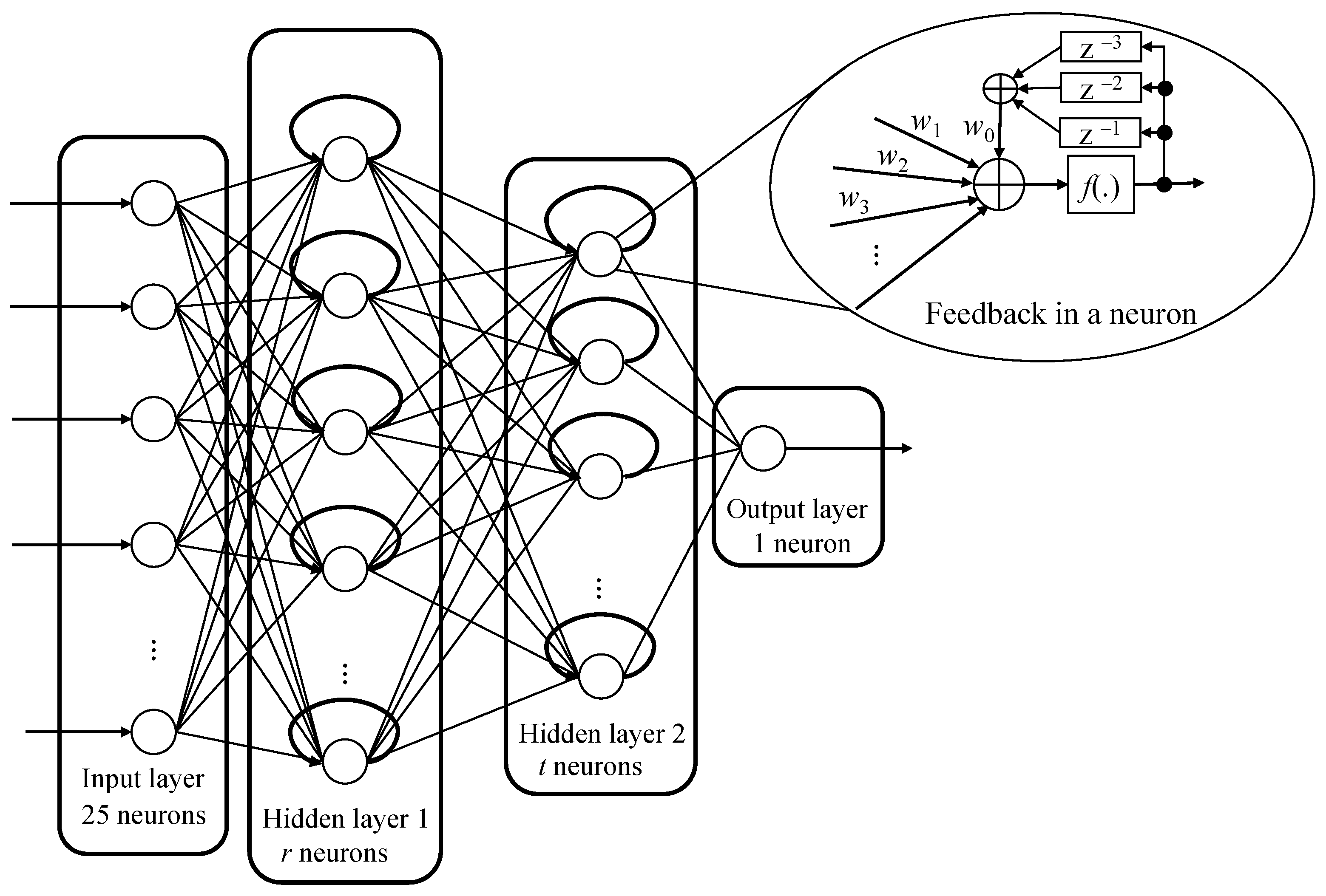
A RNN was applied to HDS systems.

-

The RNN was designed to achieve the optimized structure of ISI or ITI estimators.

-

Analysis of the RNN equalizer to estimate ISI and ITI is presented.

-

Finally, the simulation results were obtained to verify the performance of the proposed model.

The remainder of this paper is presented as follows. In Section 2, we introduce the background of the GPT target and ITI/ISI estimator. In Section 3, the proposed model is analyzed and explained. The simulation results are presented in Section 4. Finally, the conclusions are provided in Section 5.

2. Background

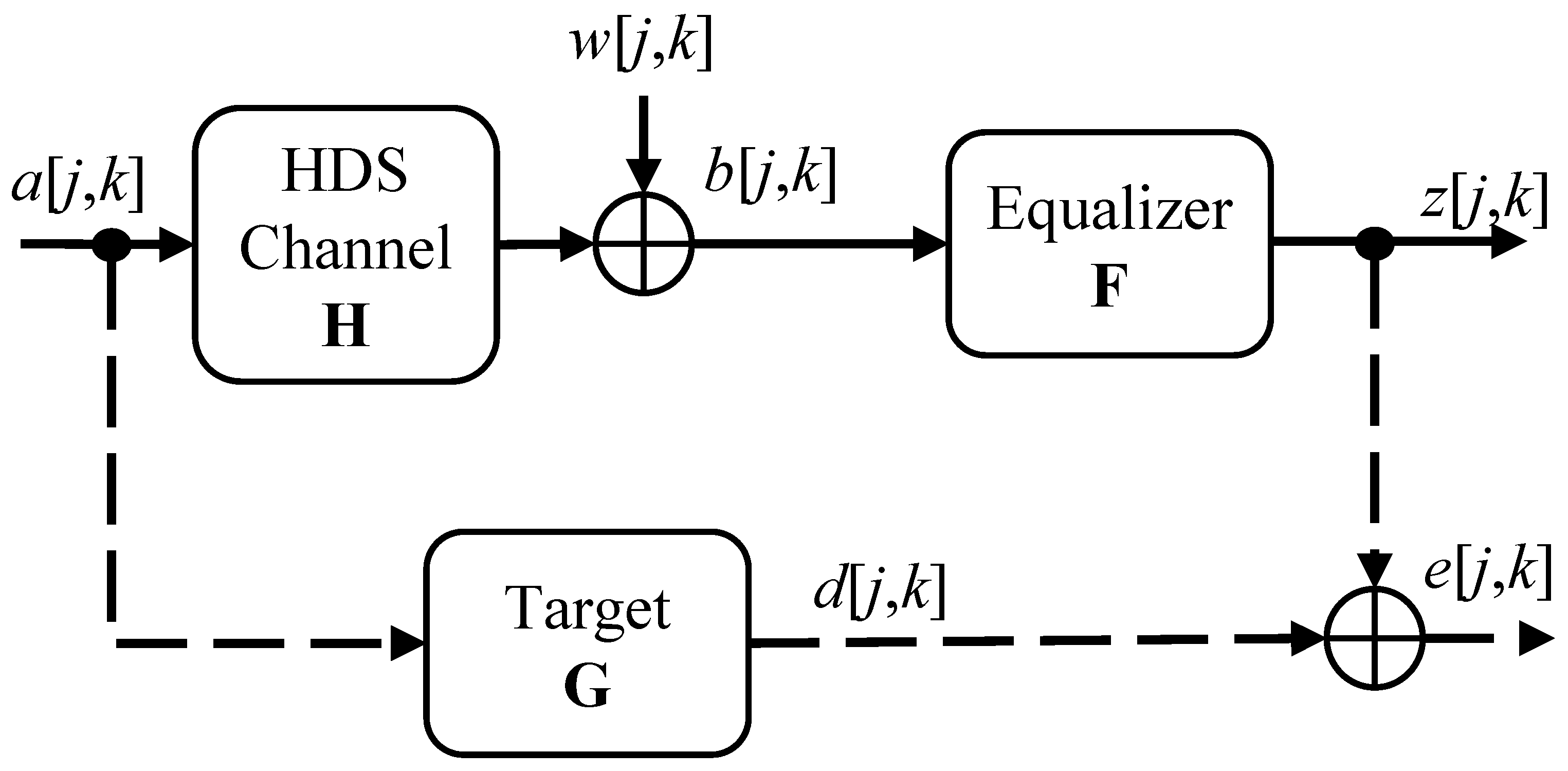
2.1. Equalizer and Generalized Partial Response Target

Figure 1 presents the structure of estimating the coefficients of equalizer F and GPR target G used in the HDS systems. a[j,k] can be represented by {−1, 1} and b[j,k] denote the modulated signal from the user data and the received signal from the HDS channel, respectively. G and F have the following matrix forms:

$$G=\left[\begin{array}{ccc}{g}_{-1,-1}& g_{-1,0}& g_{-1,1}\\ g_{0,-1}& g_{0,0}& g_{0,1}\\ g_{1,-1}& g_{1,0}& g_{1,1}\end{array}\right],\mathrm{and}$$

(1)

$$F=\left[\begin{array}{ccccc}{f}_{-2,-2}& f_{-2,-1}& f_{-2,0}& f_{-2,1}& f_{-2,2}\\ f_{-1,-2}& f_{-1,-1}& f_{-1,0}& f_{-1,1}& f_{-1,2}\\ f_{0,-2}& f_{0,-1}& f_{0,0}& f_{0,1}& f_{0,2}\\ f_{1,-2}& f_{1,-1}& f_{1,0}& f_{1,1}& f_{1,2}\\ f_{2,-2}& f_{2,-1}& f_{2,0}& f_{2,1}& f_{2,2}\end{array}\right]\hspace{0.17em},$$

(2)

Based on the method in [17], we obtained the elements of G and F using the following expressions:

$$\delta ={\left({\mathbf{C}}^T{\left(\mathbf{A}-{\mathbf{T}}^T{\mathbf{B}}^{-1}\mathbf{T}\right)}^{-1}\mathbf{C}\right)}^{-1}\alpha ,$$

(3)

$$g={\left(\mathbf{A}-{\mathbf{T}}^T{\mathbf{B}}^{-1}\mathbf{T}\right)}^{-1}\mathbf{C}\delta ,\mathrm{and}$$

(4)

$$\mathbf{f}={\mathbf{B}}^{-1}\mathbf{Tg}.$$

(5)

where A = E{aa^T}, B = E{bb^T}, and T = E{ba^T}. $\delta$ is a vector containing the Lagrange multipliers. a and b are vectors of the signal a[j,k] and b[j,k], respectively. Finally, g and f are the vectors of matrices G and F, respectively.

The matrix C and constant $\alpha$ are defined in the following equations [16]:

$$C^T=\left[\begin{array}{ccccccccc}0& 0& 0& 0& 1& 0& 0& 0& 0\end{array}\right],$$

(6)

$$\alpha =0.85.$$

(7)

This paper represents the HDS channel using the point spread function that is explained in Section 4.1. Regularly, we choose a size of 3 × 3 array pixels for the HDS channel because the channel coefficients outside the 3 × 3 array are approximately 0. Therefore, for the equalizer and detection, we set the sizes of the equalizer and target as 5 × 5 and 3 × 3, respectively.

2.2. ISI and ITI Estimator

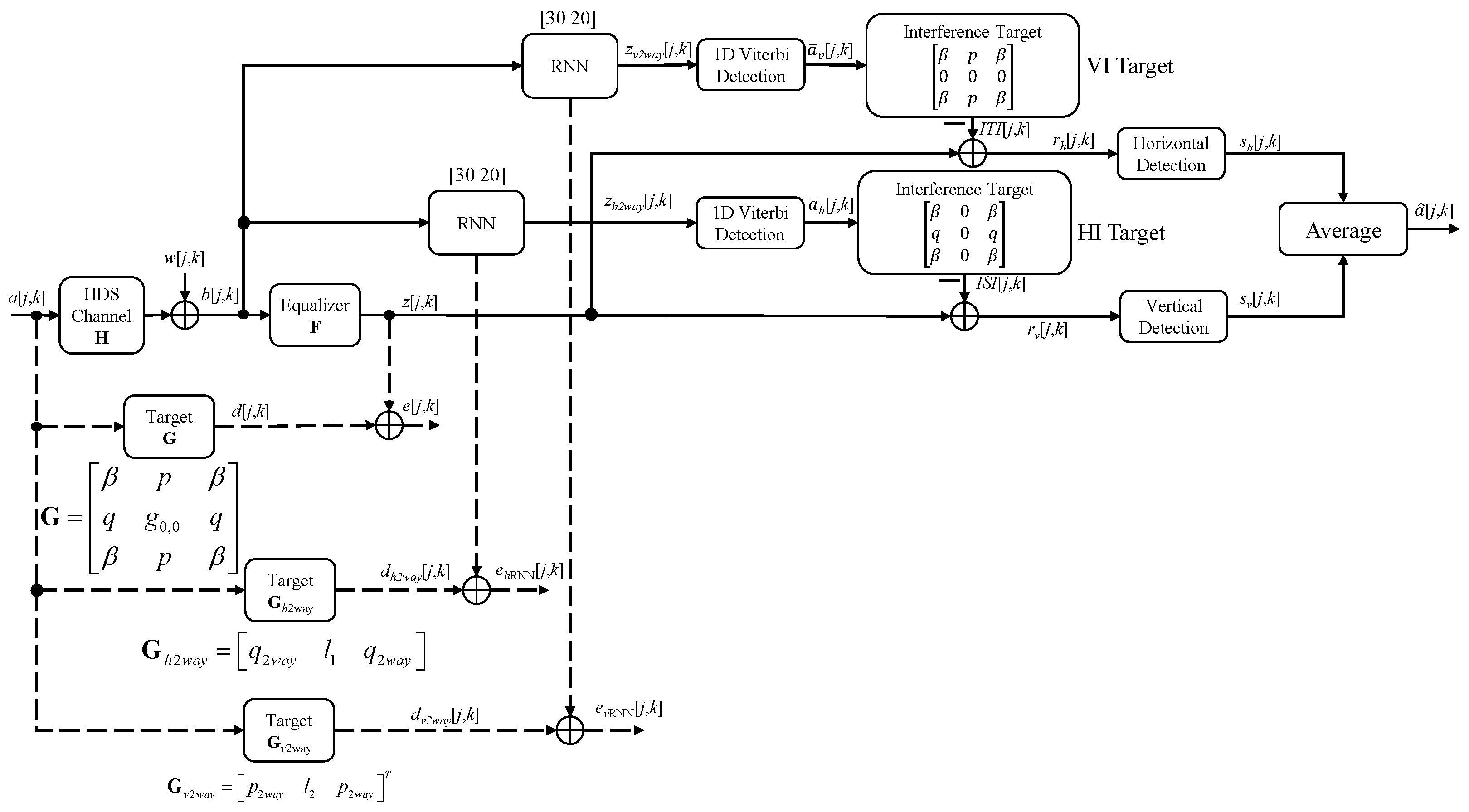
We considered the desired signal d[j,k] in Figure 1 as follows:

$$d\left[j,k\right]={\displaystyle \sum _{m=-1}^1{\displaystyle \sum _{n=-1}^{1}a\left[j-m,k-n\right]g_{m,n}}}.$$

(8)

With the 2D ISI in the HDS channel, we can achieve g_0,−1 = g_0,1 = q, g_−1,0 = g_1,0 = p, and g_1,−1 = g_−1,−1 = g_1,−1 = g_1,1 = $\beta$ as the interferences from the horizontal, vertical, and diagonal directions, respectively. We replaced q, p, and $\beta$ in (8) as follows:

$$\begin{array}{l}d\left[j,k\right]={\displaystyle \sum _{m=-1}^1{\displaystyle \sum _{n=-1}^{1}a\left[j-m,k-n\right]g_{m,n}}}\\ =a\left[j+1,k+1\right]\beta +a\left[j+1,k\right]p+a\left[j+1,k-1\right]\beta \\ +a\left[j,k+1\right]q+a\left[j,k\right]g_{0,0}+a\left[j,k-1\right]q\\ +a\left[j-1,k+1\right]\beta +a\left[j-1,k\right]p+a\left[j-1,k-1\right]\beta \end{array}.$$

(9)

In Equation (9), [$\beta$ q $\beta$]^T, [$\beta$ p $\beta$], [q g_0,0 q], and [p g_0,0 p]^T are assigned as the left-right interference (LRI), upper-lower interference (ULI), HI, and VI, respectively. In addition, the terms in (9) can be grouped into vectors as follows:

$$\left[\begin{array}{ccc}n\left[j,k+1\right]& n\left[j,k\right]& n\left[j,k-1\right]\end{array}\right],$$

(10)

where

$$n\left[j,k+1\right]=a\left[j+1,k+1\right]\beta +a\left[j,k+1\right]q+a\left[j-1,k+1\right]\beta ,$$

(11)

$$n\left[j,k\right]=a\left[j+1,k\right]p+a\left[j,k\right]g_{0,0}+a\left[j-1,k\right]p,\mathrm{and}$$

(12)

$$n\left[j,k-1\right]=a\left[j+1,k-1\right]\beta +a\left[j,k-1\right]q+a\left[j-1,k-1\right]\beta .$$

(13)

Because we used {−1, 1} to represent the signal a[j,k], n[j,k + 1], n[j,k], and n[j,k—1] have six values. With six values of n[j,k], the trellis can be used to detect n[j,k]. The LRI was then calculated as follows:

$$LRI[j,k]=n\left[j,k+1\right]+n\left[j,k-1\right],$$

(14)

Similarly, we can group the terms in (13) as follows:

$${\left[\begin{array}{ccc}m\left[j+1,k\right]& m\left[j,k\right]& m\left[j-1,k\right]\end{array}\right]}^T,$$

(15)

where

$$m\left[j+1,k\right]=a\left[j+1,k+1\right]\beta +a\left[j+1,k\right]p+a\left[j+1,k-1\right]\beta ,$$

(16)

$$m\left[j,k\right]=a\left[j,k+1\right]q+a\left[j,k\right]g_{0,0}+a\left[j,k-1\right]q,\mathrm{and}$$

(17)

$$m\left[j-1,k\right]=a\left[j-1,k+1\right]\beta +a\left[j-1,k\right]p+a\left[j-1,k-1\right]\beta .$$

(18)

Using Equation (15), after m[j,k] is detected, the ULI can be calculated as follows:

$$ULI[j,k]=m\left[j+1,k\right]+m\left[j-1,k\right],$$

(19)

3. Proposed Model

In the proposed model, we used an RNN instead of the Viterbi algorithm in [20] to estimate the LRI and ULI. The model is illustrated in Figure 2.

We used the RNN structure shown in Figure 3. It includes an input layer, two hidden layers, and an output layer. Because the received signal b[j,k] is used as the vector y, we created 25 neurons in the input layer. We designed m and n neurons in hidden layers 1 and 2, respectively, and used a neuron in the output layer. To select r and t, we implemented a simulation by varying their values. In this experiment, we simulated the horizontal detection branch of the model, as shown in Figure 2. The results are summarized in

Table 1. BER performance of RNN with varying [r t].

[r t]	14 dB	15 dB
[10 20]	0.00162	0.00093
[20 20]	0.00112	0.00043
[30 20]	0.0006	0.0002
[40 40]	0.003	0.0015

. Based on the performance shown in Table 1, we selected r = 30 and t = 20 to obtain the best BER performance. To create a feedback line for each neuron, we used three delay terms: z⁻¹, z⁻², and z⁻³. With feedback lines in the neurons, an RNN is an advantageous technique for processing sequential data. Similar to the 2D data received from the output channel, the RNN has memory to store the previous state information. Therefore, it can provide better predictions than the previous model. In addition, we used the hyperbolic tangent function for the activation function f(x) = 2/(1 + exp(−2x))−1.

In Figure 2, to create the signal a[j,k], the user signal u[k] is modulated. Subsequently, a[j,k] is stored in the HDS channel. The readback signal from HDS is b[j,k], which is distorted by the 2D interference and Gaussian noise w[j,k]. The received signal b[j,k] was supplied in three parts. The first is the equalizer part, which converts b[j,k] into z[j,k]. Signal z[j,k] is approximate to the desired signal d[j,k], which is interfered with by the 2D target G. The second is the RNN with horizontal detection creating the signal z_v2way[j,k]. Signal z_v2way[j,k] is similar to the desired signal d_v2way[j,k], which is interfered with by the 1D target G_v2way. The third is the RNN with vertical detection. Signal z_h2way[j,k] is approximate to the desired signal d_h2way[j,k], which is interfered with by the 1D target G_h2way. After the RNN converts the received y[j,k] into signals z_v2way[j,k] and z_h2way[j,k], which include 1D interference, we can use the conventional 1D VA to detect z_v2way[j,k] and z_h2way[j,k] in $\overline{a}$_v[j,k] and $\overline{a}$_h[j,k], respectively. Thereafter, the signals $\overline{a}$_v[j,k] and $\overline{a}$_h[j,k] pass through the VI and HI targets to achieve the estimated signals of the ULI and LRI, respectively, as follows:

$$\begin{array}{cc}\hfill ULI[j,k]& =\overline{a}\left[j+1,k+1\right]\beta +\overline{a}\left[j+1,k\right]p+\overline{a}\left[j+1,k-1\right]\beta \hfill \\ & +\overline{a}\left[j-1,k+1\right]\beta +\overline{a}\left[j-1,k\right]p+\overline{a}\left[j-1,k-1\right]\beta \hfill \end{array},$$

(20)

$$\begin{array}{ccc}\hfill LRI[j,k]& =\overline{a}\left[j+1,k+1\right]\beta \hfill & +\overline{a}\left[j+1,k-1\right]\beta \hfill \\ & +\overline{a}\left[j,k+1\right]q\hfill & +\overline{a}\left[j,k-1\right]q\hfill \\ & +\overline{a}\left[j-1,k+1\right]\beta \hfill & +\overline{a}\left[j-1,k-1\right]\beta \hfill \end{array}.$$

(21)

After equalizing the received signal b[j,k] into z[j,k], we can present the signal z[j,k] as follows:

$$\begin{array}{cccc}\hfill z[j,k]& \approx d\left[j,k\right]\hfill & & \\ & \approx a\left[j+1,k+1\right]\beta \hfill & +a\left[j+1,k\right]p\hfill & +a\left[j+1,k-1\right]\beta \hfill \\ & +a\left[j,k+1\right]q\hfill & +a\left[j,k\right]g_{0,0}\hfill & +a\left[j,k-1\right]q\hfill \\ & +a\left[j-1,k+1\right]\beta \hfill & +a\left[j-1,k\right]p\hfill & +a\left[j-1,k-1\right]\beta \hfill \end{array}.$$

(22)

Next, we can remove ULI[j,k] or LRI[j,k] from the signal z[j,k] as follows:

-

Removing ULI[j,k]:

$$\begin{array}{cccc}\hfill z[j,k]-ULI\left[j,k\right]& \approx a\left[j+1,k+1\right]\beta \hfill & +a\left[j+1,k\right]p\hfill & +a\left[j+1,k-1\right]\beta \hfill \\ & +a\left[j,k+1\right]q\hfill & +a\left[j,k\right]g_{0,0}\hfill & +a\left[j,k-1\right]q\hfill \\ & +a\left[j-1,k+1\right]\beta \hfill & +a\left[j-1,k\right]p\hfill & +a\left[j-1,k-1\right]\beta \hfill \\ & -\overline{a}\left[j+1,k+1\right]\beta \hfill & -\overline{a}\left[j+1,k\right]p\hfill & -\overline{a}\left[j+1,k-1\right]\beta \hfill \\ & -\overline{a}\left[j-1,k+1\right]\beta \hfill & -\overline{a}\left[j-1,k\right]p\hfill & -\overline{a}\left[j-1,k-1\right]\beta \hfill \end{array}.$$

(23)

-

Removing LRI[j,k]:

$$\begin{array}{cccc}\hfill z[j,k]-LRI\left[j,k\right]& \approx a\left[j+1,k+1\right]\beta \hfill & +a\left[j+1,k\right]p\hfill & +a\left[j+1,k-1\right]\beta \hfill \\ & +a\left[j,k+1\right]q\hfill & +a\left[j,k\right]g_{0,0}\hfill & +a\left[j,k-1\right]q\hfill \\ & +a\left[j-1,k+1\right]\beta \hfill & +a\left[j-1,k\right]p\hfill & +a\left[j-1,k-1\right]\beta \hfill \\ & -\overline{a}\left[j+1,k+1\right]\beta \hfill & & -\overline{a}\left[j+1,k-1\right]\beta \hfill \\ & -\overline{a}\left[j,k+1\right]q\hfill & & -\overline{a}\left[j,k-1\right]q\hfill \\ & -\overline{a}\left[j-1,k+1\right]\beta \hfill & & -\overline{a}\left[j-1,k-1\right]\beta \hfill \end{array}.$$

(24)

Since a[j,k] is approximated by $\overline{a}$[j,k], we can rewrite (27) and (28) as follows:

$$z[j,k]-ULI\left[j,k\right]\approx a\left[j,k+1\right]q+a\left[j,k\right]g_{0,0}+a\left[j,k-1\right]q,$$

(25)

$$z[j,k]-LRI\left[j,k\right]\approx a\left[j+1,k\right]p+a\left[j,k\right]g_{0,0}+a\left[j-1,k\right]p.$$

(26)

From (25) and (26), 1D VA can be used to detect the signal a[j,k] with the parameters [q g_0,0 q] for horizontal detection and [p g_0,0 p]^T for vertical detection. To use the average function, we applied SOVA for the horizontal and vertical detections. After the detected signal $\widehat{a}$[j,k] was demodulated into user signal $\widehat{u}$[k], we compared signals u[k] and $\widehat{u}$[k] to calculate the BER performance.

4. Simulation

4.1. HDS Channel Model

We used the channel model in [16] to set up the HDS channel. The received signal b[j,k] was obtained from the HDS channel as follows:

$$b\left[j,k\right]=a\left[j,k\right]\otimes h\left[j,k\right]+w\left[j,k\right],$$

(27)

where h[j,k] is the point spread function (PSF) of the 2D ISI and $\otimes$ is the 2D convolution operator. h[j,k] of the HDS channel can be calculated as follows:

$$h\left[j,k\right]={\displaystyle \underset{j-\frac{1}{2}}{\overset{j+\frac{1}{2}}{\int }}{\displaystyle \underset{k-\frac{1}{2}}{\overset{k+\frac{1}{2}}{\int }}h\left(x,y\right)dxdy}},$$

(28)

where h(x,y) is the continuous PSF and defined as

$$h\left(x,y\right)=\frac{1}{{\sigma }_b^2}\sin c^2\left(\frac{x-m_x}{{\sigma }_b},\frac{y-m_y}{{\sigma }_b}\right);$$

(29)

${\sigma }_b$ is the blur grade; m_x is the misalignments in the horizontal direction; m_y is the misalignments in the vertical direction; and sinc(x,y) = (sin($\pi$x)/$\pi$x)(sin($\pi$y)/$\pi$y). In this study, h[j,k] has a size of 3 × 3 array pixels. Finally, w[j,k] is the additive white Gaussian noise (AWGN) with zero mean and variance ${\sigma }_w^2$. In addition, the SNR is defined as follows:

$$\mathrm{SNR}=10{\log }_{10}\left(\frac{1}{{\sigma }_w^2}\right),$$

(30)

4.2. Simulation Results

To implement the model in Figure 2, we had to first estimate the GPR target and equalizer and train the RNN. We created the user data u[k] with 1,440,000 bits, and the probabilities of bits 0 and 1 were identical. u[k] was modulated into a 2D data page a[j,k] (1200 × 1200 bits). One page was used in estimating the GPR target and equalizer. The signal a[j,k] was distorted as in (27) and created the signal b[j,k]. The signals a[j,k] and b[j,k] were collected and converted into the vectors a and b in Section 2. Using (3)–(5), we obtained the GPR target G and equalizer F. For the RNN in the first branch, the signals a[j,k] and b[j,k] were also collected and used to estimate G_h2way. Then, with G_h2way, we calculated the signal d_h2way[j,k], using b[j,k] as the input and d_h2way[j,k] as the label to train the RNN in Section 3. Similarly, for the RNN in the second branch, G_v2way was estimated from a[j,k] and b[j,k]. The signal d_v2way[j,k] was calculated from a[j,k] and G_v2way. The RNN was trained with the input b[j,k] and label d_v2way[j,k]. In addition, to achieve the matrices G_h2way and G_v2way, we applied the below conditions.

-

Conditions of G_h2way:

$$C^T=\left[\begin{array}{ccccccccc}1& 0& 0& 0& 0& 0& 0& 0& 0\\ 0& 1& 0& 0& 0& 0& 0& 0& 0\\ 0& 0& 1& 0& 0& 0& 0& 0& 0\\ 0& 0& 0& 0& 1& 0& 0& 0& 0\\ 0& 0& 0& 0& 0& 0& 1& 0& 0\\ 0& 0& 0& 0& 0& 0& 0& 1& 0\\ 0& 0& 0& 0& 0& 0& 0& 0& 1\end{array}\right],$$

(31)

$$\alpha ={\left[\begin{array}{ccccccc}0& 0& 0& 0.85& 0& 0& 0\end{array}\right]}^T.$$

(32)

-

Conditions of G_v2way:

$$C^T=\left[\begin{array}{ccccccccc}1& 0& 0& 0& 0& 0& 0& 0& 0\\ 0& 0& 1& 0& 0& 0& 0& 0& 0\\ 0& 0& 0& 1& 0& 0& 0& 0& 0\\ 0& 0& 0& 0& 1& 0& 0& 0& 0\\ 0& 0& 0& 0& 0& 1& 0& 0& 0\\ 0& 0& 0& 0& 0& 0& 1& 0& 0\\ 0& 0& 0& 0& 0& 0& 0& 0& 1\end{array}\right],$$

(33)

$$\alpha ={\left[\begin{array}{ccccccc}0& 0& 0& 0.85& 0& 0& 0\end{array}\right]}^T.$$

(34)

To test our model, we created 10 pages. The signal a[j,k] was passed through the HDS channel to create the signal b[j,k]. The signal b[j,k] was supplied to two RNNs and equalizer F to create the signals z[j,k], z_h2way[j,k], and z_v2way[j,k]. Then, z_h2way[j,k] and z_v2way[j,k] were handled as in Section 3 to obtain the ISI[j,k] and ITI[j,k]. We mitigated ITI[j,k] from z[j,k] to create r_h[j,k]. Simalarly, to create r_v[j,k], ISI[j,k] was subtracted from z[j,k]. r_h[j,k] and r_v[j,k] were detected by 1D VA following horizontal and vertical directions to create the signals s_h[j,k] and s_v[j,k], respectively. s_h[j,k] and s_v[j,k] were put through the average function to achieve the signal $\widehat{a}$[j,k]. $\widehat{a}$[j,k] was restored into the original signal $\widehat{u}$[k] using demodulation. Subsequently, we counted the error bits (different bits between u[k] and $\widehat{u}$[k]) to calculate the BER performance. We set up a dataset with 60% training and 40% validation data and trained the RNN with 100 epochs. Figure 4 and Figure 5 show the learning curves of the RNNs in the horizontal and vertical detection branches, respectively. Finally, we used the mean square error (MSE) as the loss function, which is calculated as below.

-

The loss function for the first RNN:

$$loss=MSE=\frac{1}{2MN}{\displaystyle \sum _{j=1}^M{\displaystyle \sum _{k=1}^N{\left(b\left[j,k\right]-d_{h2way}\left[j,k\right]\right)}^2}},$$

(35)

-

The loss function for the second RNN:

$$loss=MSE=\frac{1}{2MN}{\displaystyle \sum _{j=1}^M{\displaystyle \sum _{k=1}^N{\left(b\left[j,k\right]-d_{v2way}\left[j,k\right]\right)}^2}},$$

(36)

where M is the number of rows and N is the number of columns of the data page b[j,k]. In our simulation, M = N = 1200.

Next, we simulated the proposed model using the testing data. We set up a blur of 1.85 and 0% misalignment. The blur was a parameter of the HDS channel. This represented the energy of the light on the project screen. When the blur increases, the energy of the light is radiated around. This leads to reduced energy and increased noise for the desired pixels. Simultaneously, the radiation makes the 2D ISI increase.

Figure 6 presents the BER performance of the output signal from the first branch, second branch, and combined branch (the average function branch). The outputs of the first and second branches are similar to the signal a[j,k]. The output of the combined branch can achieve a gain of 2 dB at a BER of 10⁻⁴. The output of the combined branch can improve the BER performance because the combined branch can balance the information from horizontal and vertical detections.

In the following simulation, we compared the proposed model with those of previous studies. Figure 7 presents an interference estimator with a parallel structure, which corresponds to the model introduced in [17]. Serial detection was implemented following the methodology outlined in [16]. Furthermore, a decision feedback equalizer (DFE) with a reliability factor was simulated as described in [27]. 2D SOVA and the 1D GPR target, which were introduced in [15], respectively, are also compared with our model. The results demonstrate that the proposed model can improve the BER performance of HDS systems. In particular, it can achieve a gain of ~1 dB at BER = 10⁻⁴ compared to the model in [17].

Next, we set up 10% misalignment of the HDS channel. Figure 8 demonstrates that the proposed model still achieves the best performance. The gain of the proposed model is 1 dB at a BER of 10⁻⁴. When increasing the misalignment, the ITI and ISI also grow. However, by estimating the increase in the ITI and ISI, our proposed model can compensate for this change and improve the BER performance of HDS systems. With 2D SOVA and 1D GPR target models, we can see that the performance changed more when increasing the misalignment because the 2D SOVA and 1D GPR target models did not have the ITI/ISI estimators.

As shown in Figure 9, we changed the blur from 1.8 to 3 with an SNR of 15 dB and misalignments of 0% and 10%. The simulation results show that our model can enhance the BER performance when the blur is less than 2.6. Therefore, our proposed model can resist the blur up to 2.6.

4.3. Complexity

To estimate the complexity of the proposed model, we counted the operators per detected bit from the equalizer to detection. The results are summarized in

Table 2. Complexity of our proposed model and previous studies.

Methods	Mul/Div	Add/Sub	Log/Exp
Our model	3053	3122	102
Interference estimator in [17]	508	1007	0
Serial detection in [16]	252	700	0
1D GPR [15]	33	48	0

, demonstrating that the proposed model can enhance the BER performance of the HDS channel; however, its complexity increases. This represents a trade-off between the performance and complexity of our proposed model.

In addition, to estimate the time for the complexity of the proposed model, we used a computer with an i5-11400 CPU, 16 GB of RAM, and GTX 1650 graphics card. In addition, we used MATLAB version 2023a to count the time for detecting one bit. The process times of the models are shown in

Table 3. Time for detecting one bit.

Methods	Time (Millisecond)
Our model	2.572
Interference estimator in [17]	0.261
Serial detection in [16]	0.1386
1D GPR [15]	0.006

.

5. Conclusions

In this article, we proposed a method for estimating the ITI or ISI using an RNN. With a pretrained RNN, the received signal from the output of the HDS channel was passed through the RNN to predict the ITI or ISI values. Simultaneously, we implemented experiments to find out the best structure for the RNN in an ITI/ISI estimator. The ITI and ISI were supplied and removed from the received signal, which are the outputs of the equalizer, with the higher accuracy. Finally, the original signal was detected using 1D SOVA. In the simulations, the results showed that our proposed model can achieve better performance than the previous studies. Compared to the VA estimator, at a BER of 10⁻⁴, our model can obtain a gain of ~1 dB. Simultaneously, under misalignment and blur conditions, the proposed model still achieves the best performance. However, because of using two RNNs for the parallel structure, the complexity must also be high to achieve this performance. Therefore, future work must develop a model to reduce the complexity by grouping two RNNs into one RNN. In addition, it is necessary to modify the structure of the RNN to achieve a simpler structure to minimize the processing time.

References

1. Hesselink, L.; Orlov, S.S.; Bashaw, M.C. Holographic data storage systems. Proc. IEEE 2004, 92, 1231–1280. [Google Scholar] [CrossRef]
2. Koo, K.; Kim, S.V.; Jeong, J.J.; Kim, S.W. Two-dimensional soft output viterbi algorithm with a variable reliability factor for holographic data storage. Jpn. J. Appl. Phys. 2013, 52, 09LE03. [Google Scholar] [CrossRef]
3. Bernal, M.-P.; Burr, G.W.; Coufal, H.; Quintanilla, M. Balancing interpixel cross talk and detector noise to optimize areal density in holographic storage systems. Appl. Opt. 1998, 37, 5377–5385. [Google Scholar] [CrossRef] [PubMed]
4. Wang, Z.; Jin, G.; He, Q.; Wu, M. Simultaneous defocusing of the aperture and medium on a spectroholographic storage system. Appl. Opt. 2007, 46, 5770–5778. [Google Scholar] [CrossRef] [PubMed]
5. Shelby, R.M.; Hoffnagle, J.A.; Burr, G.W.; Jefferson, C.M.; Bernal, M.-P.; Coufal, H.; Grygier, R.K.; Günther, H.; Macfarlane, R.M.; Sincerbox, G.T. Pixel-matched holographic data storage with megabit pages. Opt. Lett. 1997, 22, 1509–1511. [Google Scholar] [CrossRef] [PubMed]
6. Burr, G.W.; Mok, F.H.; Psaltis, D. Angle and space multiplexed holographic storage using the 90° geometry. Opt. Commun. 1995, 117, 49–55. [Google Scholar] [CrossRef]
7. Yu, F.T.; Wu, S.; Mayers, A.W.; Rajan, S. Wavelength multiplexed reflection matched spatial filters using LiNbO3. Opt. Commun. 1991, 81, 343–347. [Google Scholar] [CrossRef]
8. Rakuljic, G.A.; Leyva, V.; Yariv, A.; Yeh, P.; Gu, C. Optical data storage by using orthogonal wavelength-multiplexed volume holograms. Opt. Lett. 1992, 17, 1473. [Google Scholar] [CrossRef]
9. Krile, T.F.; Hagler, M.O.; Redus, W.D.; Walkup, J.F. Multiplex holography with chirp-modulated binary phase-coded reference-beam masks. Appl. Opt. 1979, 18, 52–56. [Google Scholar] [CrossRef]
10. Ford, J.E.; Fainman, Y.; Lee, S.H. Array interconnection by phase-coded optical correlation. Opt. Lett. 1990, 15, 1088–1090. [Google Scholar] [CrossRef]
11. Cideciyan, R.; Dolivo, F.; Hermann, R.; Hirt, W.; Schott, W. A PRML system for digital magnetic recording. IEEE J. Sel. Areas Commun. 1992, 10, 38–56. [Google Scholar] [CrossRef]
12. Kim, J.; Lee, J. Two-Dimensional SOVA and LDPC Codes for Holographic Data Storage System. IEEE Trans. Magn. 2009, 45, 2260–2263. [Google Scholar] [CrossRef]
13. Nguyen, C.; Lee, J. Iterative detection supported by extrinsic information for holographic data storage systems. Electron. Lett. 2015, 51, 1857–1859. [Google Scholar] [CrossRef]
14. Nguyen, C.; Lee, J. Iterative readback-aided detection for holographic data storage systems. Electron. Lett. 2016, 52, 1436–1438. [Google Scholar] [CrossRef]
15. Nabavi, S.; Kumar, B.V.K.V. Two-dimensional generalized partial response equalizer for bit-patterned media. In Proceedings of the IEEE International Conference on Communications, Glasgow, UK, 24–28 June 2007; pp. 6249–6254. [Google Scholar] [CrossRef]
16. Nguyen, T.A.; Lee, J. Simplified Two-Dimensional Generalized Partial Response Target of Holographic Data Storage Channel. Appl. Sci. 2022, 12, 4070. [Google Scholar] [CrossRef]
17. Nguyen, T.A.; Lee, J. Two-dimensional interference estimator with parallel structure for holographic data storage channel. Appl. Sci. 2022, 12, 2112. [Google Scholar] [CrossRef]
18. Nguyen, C.D.; Lee, J. 8/10 two-dimensional modulation code for holographic data storage systems. Electron. Lett. 2016, 52, 710–712. [Google Scholar] [CrossRef]
19. Hoang, H.A.; Yoo, M. 3ONet: 3-D Detector for Occluded Object under Obstructed Conditions. IEEE Sens. J. 2023, 23, 18879–18892. [Google Scholar] [CrossRef]
20. Shaoshuai, S.; Zhe, W.; Jianping, S.; Xiaogang, W.; Hongsheng, L. From points to parts: 3d object detection from point cloud with part-aware and part-aggregation network. IEEE Trans. Pattern Anal. Mach. Intell. 2021, 43, 2647–2664. [Google Scholar]
21. Duong, M.-T.; Hong, M.-C. EBSD-Net: Enhancing Brightness and Suppressing Degradation for Low-light Color Image using Deep Networks. In Proceedings of the 2022 IEEE International Conference on Consumer Electronics-Asia (ICCE-Asia), Yeosu, Republic of Korea, 26–28 October 2022; pp. 1–4. [Google Scholar] [CrossRef]
22. Wang, W.; Wu, X.; Yuan, X.; Gao, Z. An Experiment-Based Review of Low-Light Image Enhancement Methods. IEEE Access 2020, 8, 87884–87917. [Google Scholar] [CrossRef]
23. Sayyafan, A.; Aboutaleb, A.; Belzer, B.J.; Sivakumar, K.; Aguilar, A.; Pinkham, C.A.; Chan, K.S.; James, A. Deep Neural Network Media Noise Predictor Turbo-Detection System for 1-D and 2-D High-Density Magnetic Recording. IEEE Trans. Magn. 2020, 57, 1–13. [Google Scholar] [CrossRef]
24. Zhang, X.; Lue, T. A RNN decoder for channel decoding under correlated noise. In Proceedings of the 2019 IEEE/CIC International Conference on Communications Workshops in China (ICCC Workshops), Changchun, China, 11–13 August 2019; pp. 30–35. [Google Scholar]
25. Khametong, A.; Rueangnetr, N.; Warisarn, C.; Koonkarnkhai, S.; Kovintavewat, P. Deep Neural Networks based Soft-Information Improvement for Two-head/Two-track Bit-Patterned Magnetic Recording. In Proceedings of the 2022 International Symposium on Intelligent Signal Processing and Communication Systems (ISPACS), Penang, Malaysia, 22–25 November 2022; pp. 1–4. [Google Scholar] [CrossRef]
26. Nguyen, C.D.; Nguyen, P.D.; Nguyen, A.T.; Pham, N.X.; Nguyen, K.D. Performance Evaluation of Neural Network-Based Channel Detection For STT-MRAM. In Proceedings of the 8th NAFOSTED Conference on Information and Computer Science (NICS), Hanoi, Vietnam, 21–22 December 2021; pp. 430–434. [Google Scholar] [CrossRef]
27. Kim, K.; Kim, S.H.; Koo, G.; Seo, M.S.; Kim, S.W. Decision feedback equalizer for holographic data storage. Appl. Opt. 2018, 57, 4056–4066. [Google Scholar] [CrossRef] [PubMed]
Figure 1. Block diagram for estimating the coefficients of target G and equalizer F [16].
Applsci 13 11125 g001
Figure 2. Proposed model.
Applsci 13 11125 g002
Figure 3. RNN model.
Applsci 13 11125 g003
Figure 4. Learning curve of the RNN model in the first branch.
Applsci 13 11125 g004
Figure 5. Learning curve of the RNN model in the second branch.
Applsci 13 11125 g005
Figure 6. BER performance of the proposed model.
Applsci 13 11125 g006
Figure 7. BER performance comparison with 0% misalignment.
Applsci 13 11125 g007
Figure 8. BER performance comparison with 10% misalignment.
Applsci 13 11125 g008
Figure 9. BER performance according to blur.
Applsci 13 11125 g009