Numerical Gas–Liquid Two-Phase Flow Regime Identification in a Horizontal Pipe Using Dynamic Pressure Data

Abstract

Gas–liquid two-phase flow is very common in industrial pipelines. Flow regime identification is the first step to design, analyze, and operate the gas–liquid system successfully. The purpose of this study is to develop a methodology for identification of a two-phase flow regime using post signal processing techniques, namely Fast Fourier Transform (FFT) and Probabilistic Density Function (PDF). Three different flow regimes were simulated in a 6 m horizontal pipe with a 0.050 m inner diameter. A Level-Set (LS) method coupled with Volume of Fluid (VOF) method is used to model the air–water interface. After validation of the numerical method, dynamic pressure readings were collected with the intent to identify the associated flow regimes by post-processing of these signals. It was concluded that dynamic pressure signals of different flow regimes show different characteristics (like dominant frequency, FFT amplitude, PDF location and PDF magnitude) in the time and frequency domains. These characteristics can be potentially used as differentiating factors to distinguish different flow regimes. This research is limited to stratified, slug, and annular flow in the horizontal pipe. This paper uses a new approach to identify the flow regime in a horizontal pipe by Fast Fourier Transform and Probability Density Function of dynamic pressure readings obtained by using numerical simulation.

1. Introduction

Flow of fluids is an important phenomenon in many industrial and physical processes. In the literature, two main kinds of flows are discussed, namely single-phase and multi-phase flow. Two-phase flow is a simpler form of multi-phase flow, which is further classified into gas–liquid [1], liquid–liquid [2], gas–solid [3], and liquid–solid flow [4]. Gas–liquid flow is the most common multiphase flow encountered in engineering systems like refrigeration, petroleum transportation, chemical processes, and heat exchangers [5,6]. Two-phase flow can be further sub-divided into different regimes based on their appearance. An investigation on issues related to flow regime identification is important because almost every relation/mechanism for two-phase fluid models depends on the flow regime. Multi-phase flow measurements like void fraction, flowrate, and fluid velocity depend on the flow regime [7,8]. The first step to design, analyze, and operate any gas–liquid two-phase flow system is the correct identification of the flow regime. Different flow regime identification methods have been presented in the literature but there is no agreement on the universality of the methods. Traditionally, subjective methods, like Close Visual Inspection (CVI), were used to identify the flow regime [9,10] in industry. This method requires the analysis to be performed within arm’s length and optical/visual access, which is not practical and feasible for site/field deployment.

Void fraction, defined as the ratio of gas volume to total volume, is a parameter that is widely used to identify flow regime/patterns. Jones and Zuber [11] measured void fraction fluctuations in air–water flow in a rectangular section using a linearized X-ray void measurement system. It was concluded that the Probabilistic Density Function (PDF) of void fraction fluctuation can be used to differentiate slug, bubbly, and annular flow. They concluded that slug flow is simply a transitional, periodic time combination of annular and bubbly flow. The method by Jones and Zuber faces some difficulties in implementation due to the use of radioactivity and complicated construction. Merilo et al. [12] used rotating electric field conductance gauge with six electrodes to measure void fraction in circular cross section for air–water two-phase flow in vertical and horizontal flow. They also used the statistical concept of PDF to study the behavior of different flow patterns. Electrical capacitance tomography [13] and conductance probes [14] are also used to identify flow regimes. All these methods, even though capable of identifying flow regimes, possess some intrinsic limitations on the range of flow regimes that can be identified. The intrusiveness in nature of some of these methods due to the placement of sensors within the flow stream could potentially alter the flow regime. Radiation absorption techniques can provide excellent results, but the use and handling of radiation sources can cause health and safety related issues, which completely defies the original purpose. The Electrical Capacitance Tomography (ECT) [15] technique is also a good alternative for flow regime identification because it is relatively inexpensive. However, its deployment is rarely seen in industries because of the cumbersome processes involved in setting up the ECT base reference for tomography.

The use of a transducer to obtain pressure signals is a more sensible approach considering pressure readings are often needed in the process train safety and their data is easily available. That is why pressure fluctuation signals are commonly used to identify two-phase flow regimes [16,17,18,19]. This method is simple, inexpensive, and requires small modification to the existing piping setup. It is suitable for both laboratory and industrial deployment. Based on literature, pressure fluctuations combined with post signal processing techniques can be used to identify different flow patterns. Elperin and Klochko [17] used differential pressure readings in a vertically installed venturi meter to identify the flow regime based on wavelet transform method. The method processes raw differential pressure signals by decomposition of these signals into several standard forms and correlates them to the energy levels and flow pattern. Mendes [20] used a high frequency pressure transducer (Validyne DP15 at 5 kHz with a cutoff frequency of 20 Hz) to measure the differential pressure signature in annular ducts for developing an approach to identify different flow regimes. The approach is based on three important parameters, dominant frequency (f_d), which is the higher energy frequency of power spectral density (PSD); mode of PDF, called P_peak: and the difference between maximum value and mode, called the dispersion measurement (𝛿). Wambsgans et al. [21] studied horizontal two-phase flow in a rectangular section and developed a flow pattern map with the help of visual observations and dynamic pressure. A comparison of the resulting flow map was made against the flow regime maps for circular pipes, capillaries, and large rectangular geometries. It was concluded that no quantitative agreement exists, and hence the same flow map cannot be applied to different geometries. Later, Cai et al. [22] further processed this data using tools like power spectral density function (PSD), pseudo-phase-plane trajectory, autocorrelation function, fractal dimensions, and Lyapunov exponents. Again, the data can be used for flow map development in rectangular sections but was not applicable for circular pipes. Another study [23] used a technique based on processing of differential pressure signals using Hilbert Huang transform (HHT) to differentiate between different flow regimes. Hilbert Huang transform was used to decompose signals into intrinsic mode functions (IMFs). The rules to identify different flow regimes were summarized from calculated energy fraction of IMFs and the mean residual value of functions. This method shows high precision in the case of slug and bubbly flow identification. Matsui [16,24] used differential pressure data of nitrogen–water flow in vertically oriented pipe and observed that the shape of PDF can be used as a differentiating factor for different flow patterns. Vieira et al. [18] further modified and generalized the methodology used by Matsui [16,24]. A signal processing approach was presented by using differential pressure measurements in slightly inclined annular ducts to characterize slug flow. A relation was established between differential pressure signals and void pressure waves, which has the potential to identify and characterize flow patterns. Hanafizadeh et al. [25] used differential pressure signals in gas–water two-phase flow in a vertical pipe and defined a flow pattern/regime identification technique by using magnitude and dominant frequency of FFT and magnitude and location of the PDF combined with artificial neural network. Shaban and Tavoularis [26] applied the elastic map algorithm and PDF of the normalized differential pressure in gas–water two-phase flow in an upwards vertical pipe to identify the flow regime. They concluded that the PDF of differential pressure is a reliable and strong indicator for flow regime identification. The elastic map method used is accurate and versatile and it can be automated. They postulated that the PDF of differential pressure signals can also be utilized to identify two-phase flow patterns in a horizontal pipe. In fact, the use of differential pressure fluctuations can be traced back to the original work of Lockhart and Martinelli [27], where parameter $X$, is defined as:

$$X=\sqrt{\frac{{\left(dp/dz\right)}_g}{{\left(dp/dz\right)}_l}}$$

(1)

The focus of the published literature is on using differential pressure signals in vertical pipes to identify the flow regime. It is known that differential pressure is basically another term for pressure difference over a certain fixed length of pipe. Practically, it is rather cumbersome to require two measurements at different locations to be defined as ‘data’. This work extends the previous work [28,29] by the same research group, which used deep learning techniques on dynamic pressure signals in horizontal pipes to identify different flow regimes. Continuous wavelet transform was used to convert pressure signals into images and then ShuffleNet and ResNet-50 architectures were applied for classification. The objective of the present work is to identify flow regime by post-processing dynamic pressure data using Fast Fourier Transform (FFT) and Probability Density Function (PDF). The different characteristics of dynamic pressure signals (like dominant frequency, FFT amplitude, PDF location and PDF magnitude) in the time and frequency domain are studied to develop a benchmark for flow regime identification. The dynamic pressure is obtained from simulation of gas–liquid flow in a horizontal pipe using the Level-Set (LS) method coupled with Volume of Fluid (VOF). This work also explains the numerical model and methodology to simulate two-phase flow and its validation in detail. The developed methodology herein will be a steppingstone for implementation of algorithms into instrumentation hardware. The presented results show that the use of post-processing of dynamic pressure fluctuation has the potential to identify flow patterns in industrial applications where visual access to flow is not possible.

2. Methodology

The Computational Fluid Dynamics method is used to obtain data for the identification of different flow regimes. The focus of study is on gas–liquid two-phase flow in a horizontal pipe.

2.1. Governing Equations

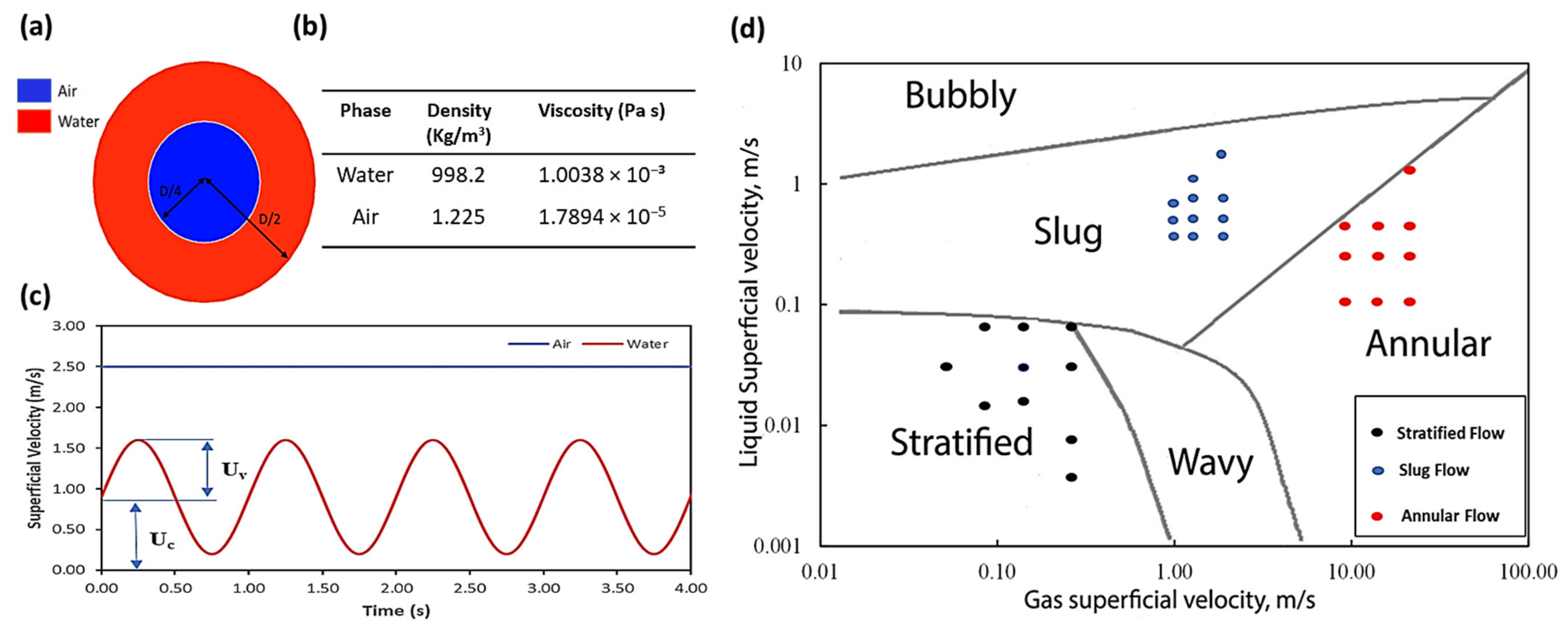
In this research, the Level-Set (LS) method coupled with the Volume of Fluid (VOF) method is used to simulate air–water two-phase flow in a horizontal pipe. Both LS and VOF methods belong to one fluid method, where a single set of conservation equations are solved. Both methods have their advantages and disadvantages, but when coupled together, the results are superior in comparison to the standalone LS or VOF method [30]. Since both methods belong to the single fluid method, there is no separated gas and liquid velocity and the continuity and momentum conservation equations are given by Equations (2) and (3), respectively. Equation (4) is used to calculate volume fraction of gas, ${\alpha }_G$. Therefore, the volume fraction of the liquid can be computed as ${\alpha }_L=1-{\alpha }_G$.

$$\frac{\partial \rho }{\partial t}+\nabla \cdot \left(\rho U\right)=0$$

(2)

$$\frac{\partial }{\partial t}(\rho U)+\nabla \cdot (\rho U\otimes U)=-\nabla p+\nabla \cdot \left[\mu (\nabla U+\nabla U^T)\right]+\rho g+F$$

(3)

$$\frac{\partial {\alpha }_G}{\partial t}+U\cdot \nabla {\alpha }_G=0$$

(4)

where t is time, U is the fluid velocity vector, ρ is fluid density, p is static pressure, μ is fluid viscosity, g is the gravitational acceleration, and F represents external body forces. Fluent evaluates body force as continuum surface force (CSF). Density and viscosity can be calculated using Equations (5) and (6).

$$\rho ={\displaystyle \sum _{k=1}^n{\alpha }_k{\rho }_k}$$

(5)

$$\mu ={\displaystyle \sum _{k=1}^n{\alpha }_k{\mu }_k}$$

(6)

For mixture turbulence equations, the realizable k-є model was used where k denotes the turbulent kinetic energy and $\epsilon$ is its rate of dissipation. The realizable k-є model differs from the standard k-є model in two important manners: it offers modified equations to evaluate dissipation rate “є” and it contains a new formulation for turbulent viscosity. The ANSYS fluent theory guide [31] reported that the realizable k-є model shows considerable improvements over other k-є models. Governing equations for the realizable turbulence model are shown in Equations (7) and (8).

$$\frac{\partial }{\partial t}\left(\rho k\right)+\nabla \cdot \left(\rho kU\right)=\nabla \cdot \left[\left(\mu +\frac{{\mu }_t}{{\sigma }_k}\right)\nabla k\right]+G_k+G_b-{\rho }_{\epsilon }-Y_M+S_k$$

(7)

$$\frac{\partial }{\partial t}\left(\rho \epsilon \right)+\nabla \cdot \left(\rho U\epsilon \right)=\nabla \cdot \left[\left(\mu +\frac{{\mu }_t}{{\sigma }_k}\right)\nabla \epsilon \right]+\rho C_1{S}_{\epsilon }-\rho C_2\frac{{\epsilon }^2}{k+\sqrt{{\upsilon }_{\epsilon }}}+C_{1\epsilon }\frac{\epsilon }{k}{C}_{3\epsilon }{G}_b+S_{\epsilon }$$

(8)

$$C_1=\max \left[0.43\frac{\eta }{\eta +5}\right]$$

(9)

$$\eta =S\frac{k}{\epsilon }$$

(10)

$$S=\sqrt{2S_{ij}{S}_{ij}}$$

(11)

“G_b” and “G_k” is the generation of turbulence kinetic energy due to the buoyancy and mean velocity gradients, respectively, “Y_M” is the contribution of dilatation to the overall dissipation rate, $"C_1,C_2,C_{1\epsilon },C_{2\epsilon }"$ are constants, while ${\sigma }_k$ and ${\sigma }_{\epsilon }$ are turbulent Prandtl numbers, S_k and $S_{\epsilon }$ are user defined source terms, $\eta$ is an expansion parameter defined by Equation (10) [31], and S_ij represents the strain rate tensor.

2.2. Geometry

The geometry used is a 6 m horizontal pipe with a 0.050 m internal diameter. The pipes inlet is divided into water and air inlets, as shown in Figure 1. Dynamic pressure readings were recorded at 81D distance from the inlet for 10 s duration. The flow is fully developed at location 81D and is recommended for both simulation [32] and experimental work [33], which was also confirmed in current simulations.

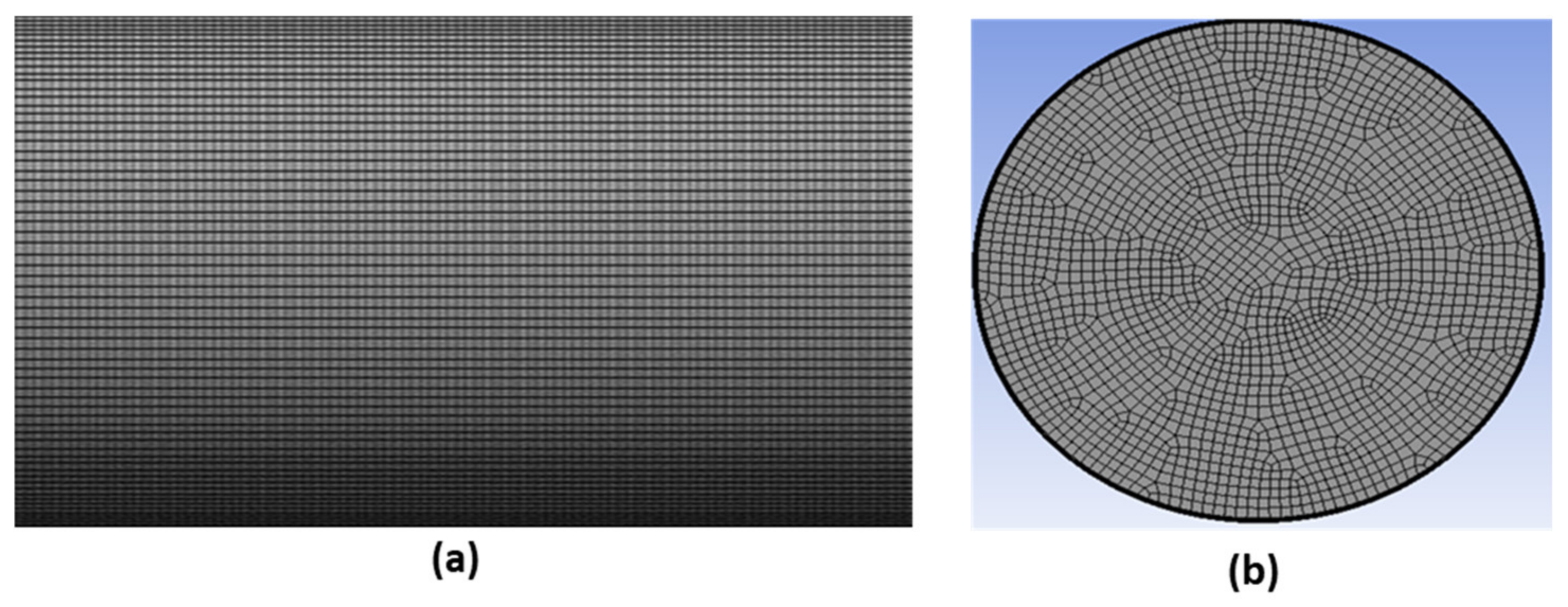
2.3. Meshing and Mesh Quality Analysis

The literature [32] shows that for straight pipes, the use of a hexahedral mesh scale decreases the computation time and increases the accuracy of solution. For that reason, the hexahedral meshing technique was used to generate the mesh. The multizone method was selected, where pure hexahedral mesh was assigned in all places possible while unstructured mesh is placed in the remaining regions, as shown in Figure 2. To capture two-phase flow behavior near the boundary walls properly and accurately, five inflation layers using the smooth transition option were applied, as shown in Figure 2b. The transition ratio used was 0.1 with a growth rate of 1.1 to get appropriate inflation layers.

The quality of the mesh is very important, and it plays a big role in stability and the accuracy of the numerical solution. The parameters used to check mesh quality are skewness, orthogonal quality, and aspect ratio. According to the definition of skewness, an equilateral cell has a value of 0 (best) and an entirely degenerate cell has value of 1 (worst). Highly skewed cells can destabilize the solution. A skewness value of 0.15 was recorded in a current study. The orthogonal quality represents how close the angles between adjoining element edges are to some optimal angle. In the case of orthogonal quality, 1 represents good and 0 represents bad quality. In the current study, the average orthogonal quality was 0.97. The ratio of the longest to shortest edge length is known as the aspect ratio. The minimum and maximum value of the aspect ratio recorded was 1.2 and 8.8, which is in a very good zone for capturing two-phase flow near the boundary layer as well as in the bulk flow region [31].

2.4. Grid Convergence Study

The selection of a proper mesh is very important in numerical studies. On one hand, choosing coarse mesh can result in a reduction in the accuracy of results, while on the other hand, choosing a very fine mesh can increase the time and cost of the simulation. Due to this reason, a grid convergence/mesh independent study was performed to find the most appropriate mesh size to be used in this study. For the grid convergence study, three different sizes of mesh were chosen, namely coarse, medium, and fine. The size of the coarse, medium, and fine meshes were 0.008, 0.005, and 0.004 m, respectively. During simulation, liquid and gas superficial velocities were kept at 2.8 m/s and 3.2 m/s. Dynamic pressure at location 1.33 m downstream was chosen as a reference point to quantify dynamic pressure for all mesh sizes.

The Grid Convergence Index (GCI) can be used to check if the results are in the asymptotic range of convergence, and it can be calculated using Equation (12). Numerical solution is closer to actual solution when grid resolution approaches zero. GCI indicates how much can a solution improves with more refinement of the mesh. A smaller GCI value shows that the use of a corresponding mesh size results in solutions that are well within range of the true numerical value.

$$\mathrm{GCI}=\frac{F\left|\epsilon \right|}{(r^p-1)}$$

(12)

$$\epsilon =\frac{f_2-f_1}{f_1}$$

(13)

$$p=\frac{\ln \left(\frac{f_3-f_2}{f_2-f_1}\right)}{\ln (r)}$$

(14)

where F, $\epsilon$, p, and f stands for factor of safety, relative error, order of convergence, and selected variable, respectively. Details regarding mesh size and dynamic pressure are shown in

Table 1. Mesh details and convergence criteria.

Mesh	Elements	Size of Element (m)	Avg. Dynamic Pressure (KPa)
Coarse	175,664	0.008	1398
Intermediate	305,254	0.005	1321
Fine	458,143	0.004	1302
		Extrapolated Values	1297.2

. Extrapolated value indicates the highest number of mesh, and it can be used to represent the true solution.

Figure 3 shows the variation in average dynamic pressure readings at the selected measurement points for different meshes. When the mesh is improved from coarse to medium, the difference between the readings is high. The GCI value for this transition is 2.2%, which is not favorable and coarse mesh is not recommended. In the case of transition from medium mesh to fine mesh, the corresponding reading did not vary a lot and GCI value is 0.5%. Hence by using fine mesh, the number of elements are increased, which will increase the simulation time and cost, while not improving the results significantly. Due to this reason, medium mesh is chosen with the number of elements equal to 305,254.

2.5. Boundry Conditions

The velocity inlet boundary condition was varied to simulate different flow regimes. Superficial velocities of gas and water at the inlet were selected using the flow regime map by Taitel and Dukler [34], as shown in Figure 4d. Figure 4a shows that the injection of both phases into the pipe was done separately. The liquid phase was injected into the pipe peripherally while the gas phase was introduced at the center region. Both phases were injected with constant superficial velocities for stratified and annular flow. To generate proper slug flow, gas superficial velocity “U_SG” was kept uniform while liquid superficial velocity “U_SL” was injected using a variable velocity profile defined by Equation (15). The notation U_c is the constant component of total velocity while U_v is the variation taking place with time (t). The U_SL varies with time in the form of the sine function, as shown in Figure 4c. It was made possible using User Defined Function (UDF). The outlet boundary condition used was outlet pressure, which was assigned an atmospheric pressure value. The boundary wall condition was set to no slip boundary and the surface tension was offset to 0.072 N/m. Air and water physical properties used are listed in Figure 4b.

$$U_{SL}=U_c+U_{v}Sin(2\pi t)$$

(15)

2.6. Simulation Model Settings

For simulation purposes, the PISO (Pressure-Implicit with Splitting of Operators) scheme for velocity-pressure coupling was used. The spatial discretization for pressure and momentum used were PRESTO (PRESsure Staggered Option) and second order upwind, respectively. The choice of first order upwind was used for turbulent kinetic energy, turbulent dissipation rate, and level set function. The under-relaxation factors for pressure, density, body forces, momentum, turbulent kinetic energy, rate turbulent viscosity, turbulent dissipation, and level set function were set to 0.3, 1, 1, 0.7, 0.8, 1, 0.8, and 0.3, respectively. All residuals were set at a value of 10⁻⁵ for convergence criteria. Due to the changing nature of multi-phase phase flow, a transient simulation with a time step of 0.001 s and total physical time of 10 s was performed. This simulation time and time step was appropriate to capture the dynamic nature of different flow regimes.

3. Validation Examples

3.1. Example 1

For validation purposes, a simulation model was developed and its findings were cross-validated against the experimental results of Hanafizadeh et al. [25]. The geometry of the validation model is a 6 m vertical pipe with a 0.050 m diameter. First, similar geometry and boundary conditions were applied during simulation. Boundary conditions were adjusted to simulate slug flow using water superficial velocity, U_SL = 1.4 m/s, and air superficial velocity U_SG = 0.5 m/s. A similar procedure of obtaining pressure readings was used; readings were obtained at 14 different locations for a total duration of 10 s at every 0.001 s interval. Hanafizadeh et al. [25] analyzed their pressure data from experiments and defined four parameters to identify the associated flow regimes. These four parameters are: (i) slope of total and inlet pressure drop $(\Delta p_T)$, (ii) pressure drop variation (𝛿), (iii) pressure amplitude (𝛾), and (iv) ratio of the pressure amplitude to the average pressure (𝛌). $\Delta p_T$ shows the pressure drop through the entire pipe length, which is caused by friction due to fluid flow. Pressure drop variation, 𝛿, shows the effect of inlet pressure drop in total pressure drop. Pressure amplitude, 𝛾, is defined as the pressure difference between highest and lowest readings divided by 2, for a particular measurement point. Every flow regime can be recognized using at least one of these parameters. For validation purposes, these parameters were calculated using the present numerical model and compared with experimental results [25] in

Table 2. Comparison of present model and Hanafizadeh et al. [25] for various pressure parameters.

Parameters	Slug Flow
	Hanafizadeh et al. [25]	Present Study	Percentage Error
𝛾 (bar)	0.092 ± 0.01	0.091	1.08%
𝛌	0.724 ± 0.10	0.753	3.85%
$\Delta p_T$	−0.056 ± 0.003	−0.057	1.75%
𝛿	−0.796 ± 0.15	−0.656	17.50%

. The difference between the findings is very small, except for 𝛿, which can be contributed to the fact that for simulation of slug flow, phase introduction at the inlet is not the same in the experimental and numerical method.

The second parameter used for comparison purposes is the acquired dominant frequency of slug flow determined by Hanafizadeh et al. [25] using FFT. Figure 5 shows a comparison on the pressure frequency spectrum between the present model and the published work. In case of slug flow [25], the reported dominant frequency range was 3–5.5 Hz, whereas the present model was from 2.6 to 5.4 Hz. The highest peak reported by [25] was 3.00 Hz, while in the present finding it is 2.62 Hz.

3.2. Example 2

For this validation example, slug frequency, which was obtained via numerical simulation, is compared against existing slug frequency correlations published in the literature. The most relevant horizontal pipe correlation is the one reported by Gregory and Scott [35]. According to their correlation, slug frequency can be calculated as:

$$f_s(\mathrm{Hz})=0.0226{\left[\frac{U_{SL}}{gD}\left(\frac{19.75}{U_M}+U_M\right)\right]}^{1.2}$$

(16)

Another correlation based on experimental work was developed by Heywood and Richardson [36]. This correlation for was developed based on 42 mm diameter pipe and its expression is given as:

$$f_s(\mathrm{Hz})=0.0434{\left[\frac{U_{SL}}{U_M}\left(\frac{2.02}{D}+\frac{U_M{}^2}{gD}\right)\right]}^{1.02}$$

(17)

Greskovich and Shrier [37] developed a correlation to calculate slug frequency based on their experimental work, which was conducted for slug flow in pipes with diameters ranging from 32 mm to 152 mm.

$$f_s(\mathrm{Hz})=0.0434{\left[\frac{U_{SL}}{U_M}\left(\frac{2.02}{D}+\frac{U_M{}^2}{gD}\right)\right]}^{1.02}$$

(18)

For validation, the purpose inlet flow conditions used were water superficial velocity, U_SL = 1.1 m/s, and air superficial velocity U_SG = 1.7 m/s.

Table 3. Comparison of slug frequency between simulation results and experimental correlations.

References	Slug Frequency (Hz)	% Error
Present model	0.968	-
[35]	0.926	4.53%
[36]	1.021	5.47%
[37]	0.930	3.92%

represents the comparison of slug frequency obtained from numerical simulations and experimental correlations. The numerical results and experimental correlations were in good agreement.

4. Results and Discussion

In this study, 30 different simulations were performed, and three different flow regimes were simulated by varying the inlet phase velocities. Pressure data was collected at 81D distance from the inlet, as mentioned in Section 2.3. In addition, depending on superficial velocities, flow takes approximately 3 to 4 s to fully develop. That is why pressure signals used for post-processing were the signals obtained after the flow was fully developed. This study shows that fluctuation in pressure occurs in all flow regimes and the amplitude of fluctuation depends on flow regime and related turbulence.

Flow morphology obtained from simulations were compared with experimental results from the literature, as shown in Figure 6. Stratified and slug flow regimes were compared against [38], and annular flow was compared against [39]. Figure 6 shows a good agreement between present contours of the liquid phase and experimental photographs. This showed that flow regimes were successfully simulated and can be used to obtain dynamic pressure data for flow regime identifications. The scale ranges from red to blue, with red representing water and blue representing air.

Figure 7 shows the void fraction readings of fully developed flow collected at a single location (81D from inlet), and it can be used as another level of data quality assurance to check that different flow regimes were developed successfully. Figure 7a shows stratified flow, in which the interface between gas and liquid is smooth and the gas phase stays on top and the liquid on the bottom due to the density difference, which is reflected consistently by the void fraction graph. Figure 7b, which looks like an electrocardiogram, shows that slug flow is characterized by the presence of Taylor bubbles and liquid slugs [40]. In the void fraction graph, the presence of liquid slugs is indicated when the pipe is filled with the liquid phase; in this study, a water void fraction value higher than 0.95 was considered the offset. Every time a slug passes by the measurement point, a peak in the void fraction value is recorded. Figure 7c shows annular flow, according to the definition [40] for this flow, liquid and gas flow as separate continuous phases, with gas phase flow in the core and the liquid phase forming a thin film along the pipe wall. The void fraction graph was drawn by collecting data on the line drawn from the bottom to the top of the pipe at a fixed location. In this case, 81D location was selected but this data can be collected at any other location as well. It can be clearly seen that at the bottom and top of pipe is filled with liquid phase (void fraction ≈ 1), whereas in the core gas phase prevails.

4.1. Flow Regime Identification

The difference in pressure properties of each flow regime makes it possible to identify flow regimes using their pressure manifestation. Pressure fluctuation and average pressure data are discussed in the following sub-sections to develop important criteria to identify different flow regimes.

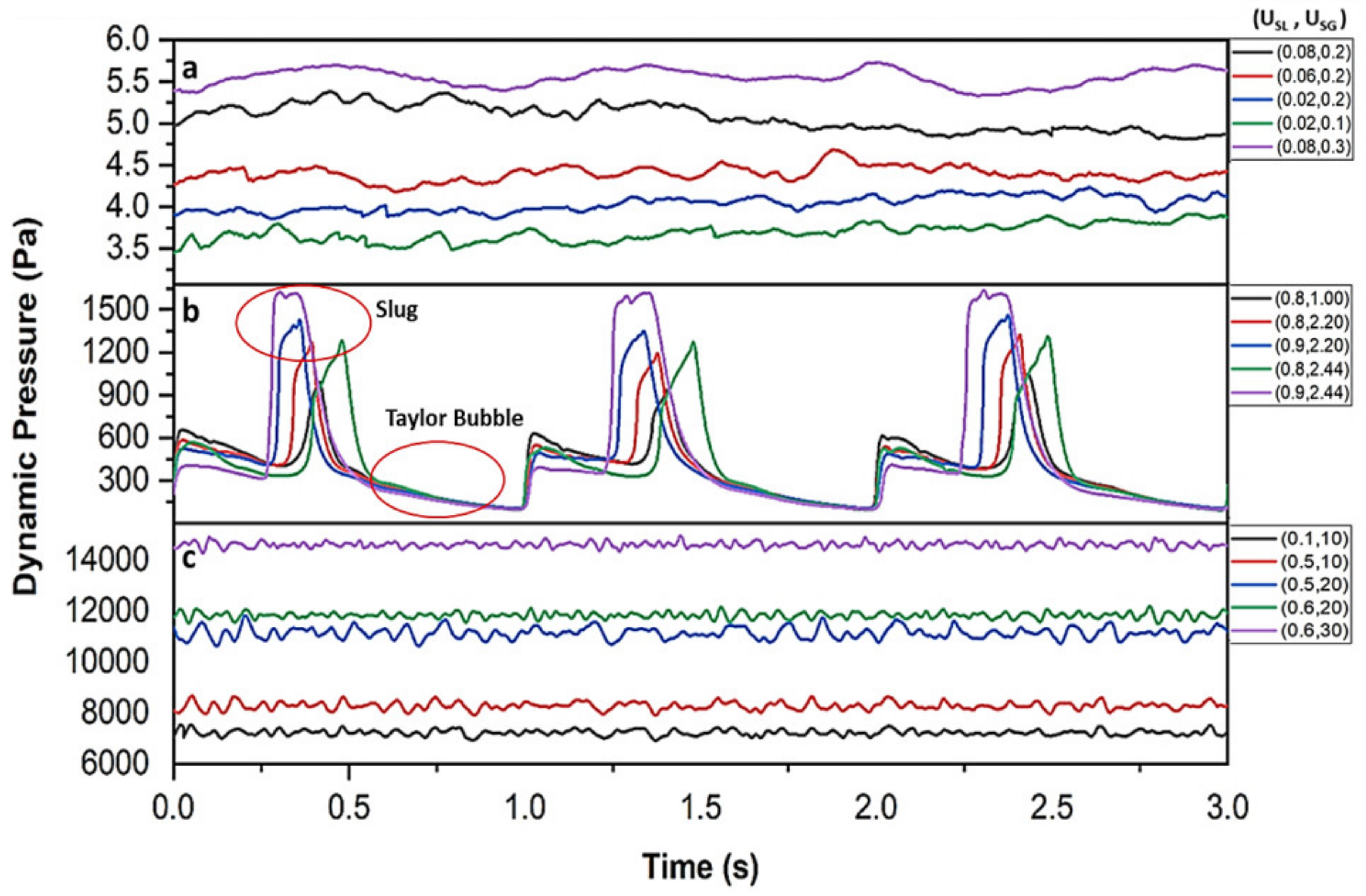
4.1.1. Pressure Fluctuations

Pressure fluctuation signals at a position located at 81D from the inlet are presented in Figure 8. All three types of flow regimes show different pressure fluctuation patterns and magnitude. Stratified flow shows negligible pressure fluctuation due to low superficial velocities and pressure amplitude increases with an increase in mixture superficial velocities. Slug flow shows considerable fluctuations compared to other flows and the magnitude of fluctuations increases with an increase in superficial velocities. Three stages of pressure variations can be observed in pressure signals when a slug is passing inside a pipe, which agrees with observations made by [41]. First, there is a sudden rise in pressure caused by acceleration of elongated bubble. The second stage is a steady drop in pressure due to the steadily falling liquid film, and the last stage is a constant lower pressure because of the tail of the slug. In annular flow, the magnitude of pressure is higher due to high velocities, but the fluctuation is considerably smaller compared to the overall pressure magnitude. Fast Fourier transform and probability density function were used to determine recognizable parameters for flow regime identification in the next section.

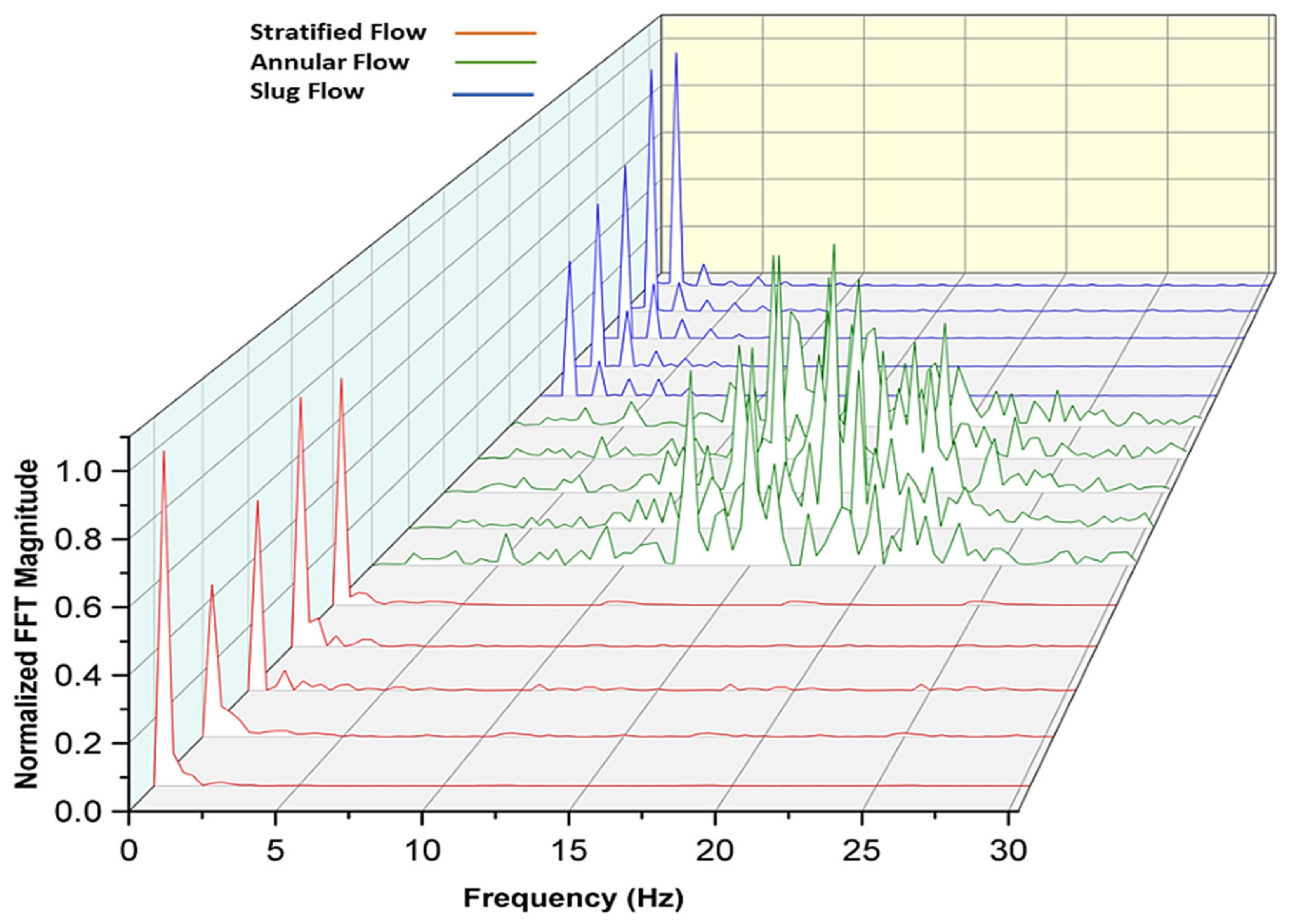
4.1.2. Fast Fourier Transformation

Fourier transformation converts the pressure signal from the time domain to the frequency domain. It is very useful in determining the dominant frequency of the signals. Figure 9 shows pressure signals in the frequency spectrum for different flow patterns. It is obvious that each flow pattern possesses its own dominant frequency range and has at least one identifiable dominant frequency where its amplitude is maximum (i.e., 1×). In the case of stratified flow, the dominant frequency is 0.33 Hz with its corresponding amplitude of 70–97 Pa. Figure 9b shows that dominant frequency for slug flow is 1.0 Hz with corresponding amplitudes ranging from 100 to 170 Pa. The smaller peaks seen are harmonics of the dominant frequency, which is the main reason they are located at multiples of the dominant frequency. Annular flow shows a dominant frequency range of 13–17 Hz, with a corresponding amplitude of 2.0–3.5 Pa. In Figure 10, the magnitude of FFT is normalized for all the recorded data for all flow regimes such that the frequencies of all flow regimes can be plotted on the same map. It is apparently evident that each flow regime forms a cluster of their own individual dominant frequency and occupies different frequency ranges. This frequency range depends on the characteristics of each flow regime and the involved distribution of phases.

Table 4. Flow regime identification criteria based on the PDF and FFT of pressure signals.

Flow Regime	Dominant Frequency FFT (Hz)	FFT Amplitude (Pa)	PDF Maximum	Location of Maximum PDF
Stratified	0.33	70–97	24–38	0.26 ± 0.02
Slug	1	100–175	1.3–1.7	0.25 ± 0.04
Annular	12.5–17	2.2–3.5	19–26	0.95 ± 0.02

summarizes the dominant frequency of different flow regimes, which can be used for flow regime identification.

4.1.3. Probability Density Function

In the probability theory, PDF is defined as a function whose value at any given point in the sample can be understood as providing a relative probability that the value of the random variable would occur. In simple terms, PDF provides the likelihood of a random variable to occur in sample space. Pressure signal is treated as the random variable in this study. Figure 11 shows the Gaussian (or Normal) probability density function of normalized pressure signals of different flow regimes. The PDF of normalized pressure signals was calculated using a standard algorithm and it shows the relative likelihood of occurrence of dominant pressure. In stratified flow, the turbulence is lower, as expected. This means that the probability of dominant pressure repetition is very high, which leads to a narrow bandwidth of PDF and high PDF value. The pressure value is also low in stratified flow due to lower velocities, which means the PDF is shifted towards the left, in the region of lower pressure values. The maximum PDF is 38, and it occurs at a normalized pressure of 0.26 ± 0.02. In slug flow, the turbulence is higher, and the probability of pressure repetition is very low, which means the bandwidth of slug flow is expected to be higher, as shown in Figure 11b. Due to a lower probability of the recurrence of dominant pressure, the resultant PDF value is also lower. In the case of slug flow, the maximum value of PDF occurs at the normalized pressure value of 0.25 ± 0.04 with a PDF value of 1.7. In annular flow, the pressure value is higher due to increased velocities, but the fluctuation is lower when compared to slug flow, which means the probability of pressure repetition is higher and PDF has a lower bandwidth and a high PDF value. Due to higher pressure values, PDF also moved towards the right side in the higher normalized pressure region. In annular flow, the maximum value of PDF occurs at 0.95 ± 0.02 with a PDF value of 26. The obtained PDF characteristics for different flow regimes are summarized in Table 4. These characteristics are different for each flow regime and are dependent on the interaction of different phases and related turbulence in different flow regimes and hence can be used to identify different flow regimes.

5. Conclusions

A detailed investigation was performed on the dynamic pressure behavior of two-phase flow in a horizontal pipe to identify parameters that can be used for flow regime identification. The method is based on using post signal processing techniques, namely Fast Fourier Transform (FFT) and Probability Density Function (PDF), to select useful parameters for flow regime identification. A simulation model was established and validated against experimental results and empirical correlations were made to simulate different flow regimes successfully and obtain dynamic pressure signals. Post processing of these signals show different characteristics in both the time and frequency domain for all three flow regimes. It was shown that different characteristics, like dominant frequency, FFT amplitude, PDF location, and PDF maximum, obtained from the FFT and PDF of dynamic pressure signals can be used to identify the flow regime successfully. Each flow regime has a specific dominant frequency range and an identifiable location and value of the PDF maximum. The use of dynamic pressure compared to other measurable properties for the identification of the flow regime offers many advantages, e.g., ease of deployment and implementation of the algorithm to existing instrumentation devices, relatively inexpensive, requires no optical access to flow, and provides no radiation or other safety concerns. The proposed method is highly recommended for industrial applications where no visual access to flow is possible and characterization is only allowed using indirect measurements like pressure signals. This work forms a steppingstone, providing the numerical foundation and pilot case for further future work in the identification of different flow patterns using simple indirect measurements. Flow pattern and pressure drop are primary functions of pipe diameter [42,43]. The next step to extend this work is investigating the effect due to different pipe diameters, covering an extended range of superficial velocities and pipe orientations, and using an artificial neural network to train the flow regime markers. At the same time, the idealization of the CFD model and its limitations are fully understood as the current research does not consider the fluid-structure interaction where the fluid pressure is transmitted to its conduit and the interaction thereof.

References

1. Triplett, K.A.; Ghiaasiaan, S.M.; Abdel-Khalik, S.I.; Sadowski, D.L. Gas–Liquid Two-Phase Flow in Microchannels Part I: Two-Phase Flow Patterns. Int. J. Multiph. Flow 1999, 25, 377–394. [Google Scholar] [CrossRef]
2. Brauner, N. Liquid-Liquid Two-Phase Flow Systems. In Modelling and Experimentation in Two-Phase Flow 2003; Springer: Vienna, Austria, 2003; pp. 221–279. [Google Scholar] [CrossRef]
3. Wang, W.; Li, J. Simulation of Gas–Solid Two-Phase Flow by a Multi-Scale CFD Approach—Of the EMMS Model to the Sub-Grid Level. Chem. Eng. Sci. 2007, 62, 208–231. [Google Scholar] [CrossRef]
4. Peker, S.M.; Helvaci, S.S. Solid-Liquid Two Phase Flow, 1st ed.; Elsevier: Amsterdam, The Netherlands, 2008; pp. 71–166. [Google Scholar]
5. Brill, J.P.; Arirachakaran, S.J. State of the Art in Multiphase Flow. J. Pet. Technol. 1992, 44, 538–541. [Google Scholar] [CrossRef]
6. Asemi, H.; Daneshgar, S.; Zahedi, R. Experimental Investigation of Gamma Stirling Refrigerator to Convert Thermal to Cooling Energy Utilizing Different Gases. Resour. Environ. Inf. Eng. 2022, 4, 200–212. [Google Scholar] [CrossRef]
7. Khan, U.; Pao, W.; Sallih, N. A Review: Factors Affecting Internal Two-Phase Flow-Induced Vibrations. Appl. Sci. 2022, 12, 8406. [Google Scholar] [CrossRef]
8. Zahedi, R.; Babaee Rad, A. Numerical and Experimental Simulation of Gas-Liquid Two-Phase Flow in 90-Degree Elbow. Alex. Eng. J. 2022, 61, 2536–2550. [Google Scholar] [CrossRef]
9. Kaichiro, M.; Ishii, M. Flow Regime Transition Criteria for Upward Two-Phase Flow in Vertical Tubes. Int. J. Heat Mass Transf. 1984, 27, 723–737. [Google Scholar] [CrossRef]
10. Taitel, Y.; Barnea, D.; Dukler, A.E. Modelling Flow Pattern Transitions for Steady Upward Gas-Liquid Flow in Vertical Tubes. AIChE J. 1980, 26, 345–354. [Google Scholar] [CrossRef]
11. Jones, O.C.; Zuber, N. The Interrelation between Void Fraction Fluctuations and Flow Patterns in Two-Phase Flow. Int. J. Multiph. Flow 1975, 2, 273–306. [Google Scholar] [CrossRef]
12. Merilo, M.; Dechene, R.L.; Cichowlas, W.M. Void Fraction Measurement With a Rotating Electric Field Conductance Gauge. J. Heat Transf. 1977, 99, 330–332. [Google Scholar] [CrossRef]
13. Wang, H.X.; Zhang, L.F. Identification of Two-Phase Flow Regimes Based on Support Vector Machine and Electrical Capacitance Tomography. Meas. Sci. Technol. 2009, 20, 114007. [Google Scholar] [CrossRef]
14. Juliá, J.E.; Liu, Y.; Paranjape, S.; Ishii, M. Upward Vertical Two-Phase Flow Local Flow Regime Identification Using Neural Network Techniques. Nucl. Eng. Des. 2008, 238, 156–169. [Google Scholar] [CrossRef]
15. Kreitzer, P.J.; Hanchak, M.; Byrd, L. Horizontal Two Phase Flow Regime Identification: Comparison Of Pressure Signature, Electrical Capacitance Tomography (ECT) and High Speed Visualization. ASME Int. Mech. Eng. Congr. Expo. Proc. 2012, 7, 1281–1291. [Google Scholar] [CrossRef]
16. Matsui, G. Identification of Flow Regimes in Vertical Gas-Liquid Two-Phase Flow Using Differential Pressure Fluctuations. Int. J. Multiph. Flow 1984, 10, 711–719. [Google Scholar] [CrossRef]
17. Elperin, T.; Klochko, M. Flow Regime Identification in a Two-Phase Flow Using Wavelet Transform. Exp. Fluids 2002, 32, 674–682. [Google Scholar] [CrossRef]
18. Vieira, S.C.; Van der Geest, C.; Fabro, A.T.; De Castro, M.S.; Bannwart, A.C. Intermittent Slug Flow Identification and Characterization from Pressure Signature. Mech. Syst. Signal Process. 2021, 148, 107148. [Google Scholar] [CrossRef]
19. Morshed, M.; Khan, M.S.; Rahman, M.A.; Imtiaz, S. Flow Regime, Slug Frequency and Wavelet Analysis of Air/Newtonian and Air/Non-Newtonian Two-Phase Flow. Appl. Sci. 2020, 10, 3272. [Google Scholar] [CrossRef]
20. Mendes, F.A.A. Estudo Experimental, Simulação Numérica e Modelagem Fenomenológica Da Separação Gravitacional de Gás No Fundo de Poços Direcionais. Ph.D. Thesis, University of São Paulo, São Carlos, Brazil, 2013. [Google Scholar]
21. Wambsganss, M.W.; Jendrzejczyk, J.A.; France, D.M. Two-Phase Flow Patterns and Transitions in a Small, Horizontal, Rectangular Channel. Int. J. Multiph. Flow 1991, 17, 327–342. [Google Scholar] [CrossRef]
22. Cai, Y.; Wambsganss, M.W.; Jendrzejczyk, J.A. Application of Chaos Theory in Identification of Two-Phase Flow Patterns and Transitions in a Small, Horizontal, Rectangular Channel. J. Fluids Eng. Trans. ASME 1996, 118, 383–390. [Google Scholar] [CrossRef]
23. Sun, B.; Zhang, H.; Cheng, L.; Zhao, Y. Flow Regime Identification of Gas-Liquid Two-Phase Flow Based on HHT. Chin. J. Chem. Eng. 2006, 14, 24–30. [Google Scholar] [CrossRef]
24. Matsui, G. Automatic Identification of Flow Regimes in Vertical Two-Phase Flow Using Differential Pressure Fluctuations. Nucl. Eng. Des. 1986, 95, 221–231. [Google Scholar] [CrossRef]
25. Hanafizadeh, P.; Eshraghi, J.; Taklifi, A. Experimental Identification of Flow Regimes in Gas—Liquid Two Phase Flow in a Vertical Pipe. Meccanica 2015, 51, 1771–1782. [Google Scholar] [CrossRef]
26. Shaban, H.; Tavoularis, S. Identification of Flow Regime in Vertical Upward Air-Water Pipe Flow Using Differential Pressure Signals and Elastic Maps. Int. J. Multiph. Flow 2014, 61, 62–72. [Google Scholar] [CrossRef]
27. Lockhart, R.W.; Martinelli, R.C. Proposed Correlation of Data for Isothermal Two-Phase Two Component Flow in Pipes. Chem. Eng. Prog. 1949, 45, 39–48. [Google Scholar]
28. Khan, U.; Pao, W.; Sallih, N.; Hassan, F. Flow Regime Identification in Gas-Liquid Two-Phase Flow in Horizontal Pipe by Deep Learning. J. Adv. Res. Appl. Sci. Eng. Technol. 2022, 27, 86–91. [Google Scholar] [CrossRef]
29. Khan, U.; Pao, W.; Sallih, N.; Hassan, F. Identification of Horizontal Gas-Liquid Two-Phase Flow Regime Using Deep Learning. CFD Lett. 2022, 14, 68–78. [Google Scholar] [CrossRef]
30. Nichita, B.A.; Zun, I. A Volume of Fluid Method for Modeling of Gas-Liquid Interface. J. Fluids Eng. 2015, 132, 081302. [Google Scholar] [CrossRef]
31. ANSYS FLUENT 13 Ansys Fluent Theory Guide; ANSYS Inc.: Canonsburg, PA, USA, 2013; Volume 15317, pp. 724–746.
32. Ban, S.; Pao, W.; Nasif, M.S. Numerical Simulation of Two-Phase Flow Regime in Horizontal Pipeline and Its Validation. Int. J. Numer. Methods Heat Fluid Flow 2018, 28, 1279–1314. [Google Scholar] [CrossRef] [Green Version]
33. Mohmmed, A.O.; Nasif, M.S.; Al-Kayiem, H.H.; Time, R.W. Measurements of Translational Slug Velocity and Slug Length Using an Image Processing Technique. Flow Meas. Instrum. 2016, 50, 112–120. [Google Scholar] [CrossRef]
34. Taitel, Y.; Dukler, A.E. A Model for Predicting Flow Regime Transitions in Horizontal and near Horizontal Gas-liquid Flow. AIChE J. 1976, 22, 47–55. [Google Scholar] [CrossRef]
35. Gregory, G.A.; Scott, D.S. Correlation of Liquid Slug Velocity and Frequency in Horizontal Cocurrent Gas-liquid Slug Flow. AIChE J. 1969, 15, 933–935. [Google Scholar] [CrossRef]
36. Heywood, N.I.; Richardson, J.F. Slug Flow of Air-Water Mixtures in a Horizontal Pipe: Determination of Liquid Holdup by γ-Ray Absorption. Chem. Eng. Sci. 1979, 34, 17–30. [Google Scholar] [CrossRef]
37. Greskovich, E.J.; Shrier, A.L. Slug Frequency in Horizontal Gas-Liquid Slug Flow. Ind. Eng. Chem. Process Des. Dev. 1972, 11, 317–318. [Google Scholar] [CrossRef]
38. Mohmmed, A. Effect of Slug Two-Phase Flow on Fatigue of Pipe. PhD Thesis, Universiti Teknologi Petronas, Seri Iskandar, Malaysia, 2016. [Google Scholar]
39. Al-Tameemi, W.T.M.; Ricco, P. Pattern-Based Pressure Drop of Air–Water Flow across a 90° Sharp Mitre Elbow. Int. J. Comput. Methods Exp. Meas. 2018, 6, 198–207. [Google Scholar] [CrossRef] [Green Version]
40. Baker, O. Design of Pipelines for the Simultaneous Flow of Oil and Gas. In Proceedings of the Fall Meeting of the Petroleum Branch of AIME, Dallas, TX, USA, 19–21 October 1953. [Google Scholar] [CrossRef]
41. Vaze, M.J.; Banerjee, J. Experimental Visualization of Two-Phase Flow Patterns and Transition from Stratified to Slug Flow. Proc. Inst. Mech. Eng. Part C J. Mech. Eng. Sci. 2011, 225, 382–389. [Google Scholar] [CrossRef]
42. Chen, L.; Tian, Y.S.; Karayiannis, T.G. The Effect of Tube Diameter on Vertical Two-Phase Flow Regimes in Small Tubes. Int. J. Heat Mass Transf. 2006, 49, 4220–4230. [Google Scholar] [CrossRef]
43. Venkatesan, M.; Das, S.K.; Balakrishnan, A.R. Effect of Diameter on Two-Phase Pressure Drop in Narrow Tubes. Exp. Therm. Fluid Sci. 2011, 35, 531–541. [Google Scholar] [CrossRef]
Figure 1. Pipe geometry.
Applsci 13 01225 g001
Figure 2. Hexahedral mesh. (a) Horizontal view, and (b) side view showing the inlet.
Applsci 13 01225 g002
Figure 3. Grid convergence study.
Applsci 13 01225 g003
Figure 4. Boundary conditions. (a) Cross section of the water and air inlet. (b) Working medium physical properties (at 20 °C). (c) Air and water superficial velocity graph at the inlet for slug flow. (d) Superficial velocities used for simulation [34].
Applsci 13 01225 g004
Figure 5. Comparison on frequency spectrum of pressure signals for slug flow between published data and the findings from the present study.
Applsci 13 01225 g005
Figure 6. Comparison of flow morphology of simulation results against experimental results from the literature for (a) stratified (USL = 0.02 m/s, USG = 0.1 m/s) [38], (b) slug (USL = 1 m/s, USG = 2.44 m/s) [38], and (c) annular flow (USL = 0.5 m/s, USG = 20 m/s) [39] regimes.
Applsci 13 01225 g006
Figure 7. Void fraction of different flow regimes. (a) Stratified flow (USL = 0.08 m/s, USG = 0.2 m/s). (b) Slug flow (USL = 0.9 m/s, USG = 2.44 m/s). (c) Annular flow (USL = 0.5 m/s, USG = 20 m/s). (d) Cross section of pipe.
Applsci 13 01225 g007
Figure 8. Pressure fluctuating signals of different flow regimes: (a) stratified, (b) slug, and (c) annular.
Applsci 13 01225 g008
Figure 9. Fast Fourier Transform of the dynamic pressure signals of different flow regimes: (a) stratified, (b) slug, and (c) annular.
Applsci 13 01225 g009
Figure 10. Fast Fourier Transform of the dynamic pressure signals of different flow regimes with normalized FFT magnitude.
Applsci 13 01225 g010
Figure 11. Probability Density Function for pressure signals of different flow regimes: (a) stratified, (b) slug, and (c) annular.
Applsci 13 01225 g011