An AMR-Based Liquid Film Simulation with Surfactant Transport Using PLIC-HF Method

Abstract

In this study, an AMR-PLIC-HF method is proposed and implemented by GPU parallel computing based on CUDA programming language and NVIDIA GPU. The present method improves the computation efficiency without compromising the accuracy and conservation of the volume. To satisfy the requirements of stencil points of the PLIC-HF method, an extended stencil computation method based on the tree-based AMR method is proposed and implemented. The Weakly Compressible Scheme (WCS) is used in the present work as a fluid solver. An evolving pressure projection method is adopted to suppress the oscillation induced by the reflection of acoustic waves. The Langmuir model is introduced into the solver to calculate surfactant transport and the Marangoni effect caused by the gradient of the interface concentration of the surfactant. The single vortex flow results verify the accuracy of the AMR-PLIC method. A single bubble rising problem with two different physical property settings is simulated. The results show good agreement with the results given by incompressible solvers. This verifies the accuracy of the two-phase flow solver including the AMR-PLIC-HF method and the WCS. The generation and rupture of liquid film by a single bubble freely rising to an interface is simulated by the present solver with a $1024\times 2048$ AMR grid as the finest resolution. This simulation successfully calculates surfactant transport and the Marangoni effect.

1. Introduction

Following the development of the numerical fluid simulation field, a wide range of fluid phenomena can now be simulated. Regarding multiphase flows, the generation and rupture of thin liquid film has attracted researchers’ interest. Thin liquid films are ubiquitous in many naturally occurring processes as well as in many industrial processes [1]. Typically, when a bubble starts rising from liquid and approaches the interface, a thin liquid film is generated by the drainage of liquid. The dynamics of this process determine the behaviors of fluid in many liquid–gas two-phase flows. Due to its practical importance, the dynamics and stability of thin liquid film have been widely researched through experiments and theoretical analyses [2,3,4,5,6,7]. However, there has been little research on the dynamics and stability of thin liquid film using numerical simulations. The difficulty of conducting liquid film simulations can be divided into several aspects.

First, in a thin liquid film simulation, the length of the problem is typically much larger than the thickness of the film, which makes it a multiscale problem. In simulations of such multiscale problems, a very-high-resolution mesh grid is required to ensure that an accurate description of the behavior of liquid film is achieved. With a uniform resolution mesh grid and CPU computing, the required memory of the computer and execution time make simulations of thin liquid film impractical. CPU programs are used in conventional numerical simulations. However, the CPU is a single processing unit that can only execute a limited number of instructions at a time. Thus, in large-scale simulations, or simulations of thin liquid film that require a high-resolution mesh grid, the efficiency of the CPU is unsatisfactory. To accelerate the computation process, GPU parallel computing can be adopted. The GPU is a specialized type of processor that was designed to handle a large number of parallel calculations simultaneously. This makes GPUs well-suited for certain types of computational tasks, such as the rendering of graphics or the performance of complex calculations for scientific simulations. The GPU can provide over 100 times more FLOPS than the CPU in large-scale simulations [8].

In the simulation of real phenomena, it is inefficient to use a uniform resolution grid in the computational domain. Normally, the resolution of the grid is determined by the size of the cells or elements that make up the grid. The size of these cells is typically chosen based on the size of the smallest features in the system being simulated as well as the desired level of simulation accuracy. For example, if a simulation is being performed to study the flow of a fluid through a complex network of pipes, the grid resolution needs to be fine enough to accurately capture the details of the pipe geometry and the flow of the fluid within the pipes. This requires the use of small grid cells in the regions of the grid that correspond to the pipes to accurately represent their shapes and sizes. However, in other regions of the grid, where the fluid flow is less complex, the grid cells can be larger, as the details of the flow are not as important. This is a basic concept of the Adaptive Mesh Refinement (AMR) method. In the 1980s, led by Berger [9], researchers proposed the AMR method to dynamically adjust the size of cells and the resolution of the grid based on the complexity of the solution with higher resolutions used in regions with rapidly changing solutions and lower resolutions in regions with relatively constant solutions. In previous work by Matsushita and Aoki, the execution time and size of the computational grids were reduced by around $90\%$ through the use of a benchmark advection problem from the interface-capturing method [10,11].

Second, a highly accurate interface capturing method for two-phase flows is required for the simulation of thin liquid films. Some numerical methods, including the volume-of-fluid (VOF) method [12], level set method [13], phase field method [14], and coupled level set and VOF (CLSVOF) method [15], can describe large amounts of interface topological deformation. Considering the good conservation of mass achieved by the phase field method and the high accuracy of the complex geometric calculation in the level set method, the previous work by Matsushita and Aoki proposed a coupled phase field and level set method that combines the advantages of the two methods [16]. The phase field method describes the interface between different phases as a diffusive interface with a certain thickness. In liquid film simulations, such a diffusive interface could bring uncertainty to the simulation and may not describe the true physics. Based on the VOF method, a piecewise linear interface calculation (PLIC) method was adopted in the present research. The PLIC method has become a widely used technique in computational fluid dynamics and has been applied to a range of problems involving the simulation of free-surface flows and complex fluid–fluid interactions [17,18,19]. We believe that the sharp interface described by the PLIC method is appropriate for use in the present simulation of liquid films. The curvature was usually calculated by level set in previous work [16,20] due to the high accuracy of this method. However, the level set was not used as the main variable to capture the interface. The calculation of the volume fraction to height function is straightforward [21,22,23]. Thus, in the present research, the interface curvature was calculated by the Height Function (HF) method. It has been reported that the spurious current [24] can be greatly decreased by the present PLIC-HF method [19].

Third, the method used to solve fluid dynamics problems needs to be considered. Derived from the mesoscopic kinetic theory of gases, the lattice Boltzmann method has developed into an effective CFD method in the past two decades and can be used for research and applications [25,26]. In contrast to the Navier–Stokes equation, which is based on macroscopic conservation law, The LBM is derived from the dynamics of fluid particles and includes collision and propagation. It is modeled by a statistical distribution function to avoid the direct tracking of each particle, as occurs in molecular dynamics methods. The most notable feature of the LBM is its explicit time advancement and local spatial dependence, which enable it to fully exploit the potential of parallel computers. Inspired by the standard LBM designed for isothermal weakly compressible fluids, weakly compressible Navier–Stokes equations can also be used to simulate incompressible flows. By introducing an isothermal state equation and ignoring density fluctuations at low Mach numbers, an independent time evolution equation of pressure can be obtained [27,28]. This hyperbolic equation of pressure can be explicitly integrated in time through a local spatial stencil. Despite the limitation of the time step size by the speed of sound, this method greatly benefits scalable calculations. Weakly compressible Navier–Stokes equations have been successfully applied to turbulent flows [29] and two-phase flows [16]. The calculation of pressure Poisson equation is necessary for incompressible Navier–Stokes solvers. This method brings instability to the computation, and convergence in large-density-ratio two-phase flow simulations is compromised. Thus, a weakly compressible scheme [16] and evolving pressure projection method [30] were used in the current simulation.

The purpose of the present research was to understand the influence of surfactant transport on the behavior of liquid film. The PLIC-HF method was used as interface capturing method and implemented on an AMR grid with extended stencil computation. The weakly compressible scheme and evolving pressure projection method was used as a fluid solver. A Langmuir model [31,32,33,34] was introduced to calculate surfactant transport and the Marangoni effect.

This paper is organized as follows. Section 2 presents the governing equations. Section 3 presents an explanation of the numerical methods. Section 4 explains the implementation of AMR on GPU. The results of two-dimensional computations and a discussion of the results are given in Section 5. The results are further discussed in Section 6, and concluding remarks are given in Section 7.

2. Governing Equations

2.1. Fluid Dynamic Equations

The isothermal Navier–Stokes equation is derived from the compressible Navier–Stokes equation [20]. Under isothermal conditions, the time evolution of temperature T is not solved and T is considered to be a constant. When the Mach number is $Ma=\frac{U}{c_s}\ll 1$, the density change is $\frac{\delta \rho }{{\rho }_0}\ll 1$. U is the typical velocity, ${\rho }_0$ is the constant density, and $c_s$ is the sound speed. Assuming the flow is weakly compressible, in the computation of a single-phase flow, the density $\rho$ is considered constant, and in the computation of a two-phase flow, the density $\rho$ is calculated from the volume fraction. In this case, the density compressibility can be ignored.

Additionally, when $Ma=\frac{U}{c_s}\ll 1$, the fluid velocity is much slower than the speed of sound, and propagation by sound waves becomes dominant, so the material derivative of pressure p can be approximated as the Eulerian time derivative of pressure p. When this approximation is adopted, it has been reported that the results of the benchmark tests approach incompressibility [27]. This approaches was adopted in the present research.

With the assumptions about the isothermal state and low Mach number, the governing equations of weakly compressible flows can be shown as

$$\frac{\partial \mathit{u}}{\partial t}+\left(\mathit{u}·\nabla \right)\mathit{u}=-\frac{1}{\rho }\nabla p+\frac{1}{\rho }\nabla ·\mathit{\tau }+\frac{1}{\rho }\mathit{F},$$

(1)

$$\frac{\partial p}{\partial t}+\left(\mathit{u}·\nabla \right)p=-\rho c_s^2\nabla ·\mathit{u}.$$

(2)

where $\mathit{F}$ represents the external forces, which include the surface tension and gravity in the present research. $\mathit{\tau }$ is the viscous stress tensor.

The speed of sound $c_s$ is set using the typical velocity and initial Mach number as

$$c_s=U/Ma$$

(3)

where U is the typical velocity. $c_s$ was given a large value in the present research to ensure that the low Mach number assumption was applicable during the simulation.

An evolving pressure projection method was included in the current research to dampen the acoustic waves in weakly compressible fluid flows [30].

2.2. Conservative PLIC-VOF Method

A conservative piecewise linear interface calculation volume-of-fluid (PLIC-VOF) method was included in the present research [35,36] where a ‘color function’ $c\left(\mathit{x}\right)$ is used to describe the fluid type. This is defined as

$$c\left(\mathit{x}\right)=\left\{\begin{array}{cc}\hfill 1\hfill & \mathrm{if}\mathit{x}\in ‘\mathrm{heavy}’\mathrm{fluid}\hfill \\ \hfill 0\hfill & \mathrm{if}\mathit{x}\in ‘\mathrm{light}’\mathrm{fluid}\hfill \end{array}\right.$$

(4)

In the VOF method, a characteristic function $\varphi$ is obtained by integrating the color function into a computational volume $\mathsf{\Omega }$:

$$\varphi =\frac{{\int }_{\mathsf{\Omega }}c\left(\mathit{x}\right)\mathrm{d}v}{{\int }_{\mathsf{\Omega }}1\mathrm{d}v}$$

(5)

This characteristic function $\varphi$ is a volume fraction and has physical constraints such as

$$0⩽\varphi ⩽1$$

(6)

which means that in the computational volume, the fluid cannot be less than empty or more than full.

The PLIC method approximates interfaces on each cell as a line in two dimensional simulations, as shown in Figure 1a. The line can be described by the following equation:

$$\mathit{n}·\mathit{x}=\alpha$$

(7)

where $\alpha$ is a constant that ensures that the volume fraction cut by the interface is exactly the $\varphi$ defined by Equation (5) [37]. In Equation (7), the interface normal vector $\mathit{n}$ is computed with the second-order mixed Youngs-centered (MYC) method [38], and $\mathit{x}$ is local coordinate defined in one cell. As shown in Figure 1b, the volume flux across the cell face is calculated by the geometric relationship to advect the reconstructed interface.

The transport equation is based on the physical nature phenomenon whereby on any material point, the fluid type does not change. It can be described by the material derivative of the color function:

$$\frac{Dc}{Dt}=\frac{\partial c}{\partial t}+\mathit{u}·\nabla c=0$$

(8)

By integrating Equation (8) into a computational volume $\mathsf{\Omega }$ and using the divergence theorem, we get

$$\frac{\partial }{\partial t}{\int }_{\mathsf{\Omega }}c\mathrm{d}v+{\oint }_{\partial \mathsf{\Omega }}c{u}_n\mathrm{d}s={\oint }_{\mathsf{\Omega }}c\nabla ·\mathit{u}\mathrm{d}v$$

(9)

By considering the definition of the volume fraction $\varphi$ in Equation (5), the transport equation can be written as

$$\frac{\partial \varphi }{\partial t}\Delta \mathsf{\Omega }+F_{net}={\oint }_{\mathsf{\Omega }}c\nabla ·\mathit{u}\mathrm{d}v$$

(10)

where $\Delta \mathsf{\Omega }\equiv {\int }_{\mathsf{\Omega }}1\mathrm{d}v$ is defined as the volume of the cell. In Equation (10), the value of the right-hand side should be zero because it is a divergence-free velocity field where $\nabla ·\mathit{u}$ is zero. However, a dimensional split method was used in the current research, which means that the flux calculation and time integration proceeded alternately in the X-direction and Y-direction. One-direction velocity is not divergence-free; thus, the right-hand side could not be simply ignored. To conserve the volume, a simplification was adopted:

$${\oint }_{\mathsf{\Omega }}c\nabla ·\mathit{u}\mathrm{d}v=c_c\frac{\partial u_d}{\partial x_d}\Delta \mathsf{\Omega }$$

(11)

where d is the Cartesian index indicating the X-direction or Y-direction, and $c_c$ is the value of the color function at the center of the cell and is defined explicitly as

$$c_c=\left\{\begin{array}{cc}\hfill 1\hfill & \mathrm{if}\varphi >1/2\hfill \\ \hfill 0\hfill & \mathrm{else}\hfill \end{array}\right.$$

(12)

The interface curvature can be calculated with an improved Height Function (HF) method [22]:

$$\kappa =\frac{H_{xx}+H_{yy}+H_{xx}{H}_y^2+H_{yy}{H}_x^2-2H_{xy}{H}_x{H}_y}{{\left(1+H_x^2+H_y^2\right)}^{3/2}}$$

(13)

where $\kappa$ is the interface curvature, H is the height function calculated by volume fractions on a $3\times 7$ or $7\times 3$ stencil, and the subscripts x and y show the partial derivatives of the height function H. This method has a high level of accuracy even when the local grid resolution is low because a local monotonicity correction is included.

In the computations of density and viscosity shown in Equation (1), the volume fraction $\varphi$ is used:

$$\begin{array}{cc}\hfill & \hfill \rho =\varphi {\rho }_h+(1-\varphi ){\rho }_l\hfill \\ \hfill & \hfill \mu =\varphi {\mu }_h+(1-\varphi ){\mu }_l\hfill \end{array}$$

(14)

where the subscripts ‘l’ and ‘h’ indicate the properties of heavy fluids and light fluids, respectively.

2.3. Level Set Advection and Re-Initialization

In the present research, the level set function $\psi$ [13,39] was used as a refinement criterion in the Adaptive Mesh Refinement (AMR) method and for some surfactant transport calculations. The level set function $\psi$ evolves over time according to the advection equation shown below:

$$\frac{\partial \psi }{\partial t}+(\mathit{u}·\nabla )\psi =0.$$

(15)

Since the Level Set function $\psi$ represents the signed distance from the interface, it has the following property:

$$|\nabla \psi |=1.$$

(16)

Due to the numerical error from long-term integration, the $|\nabla \psi |=1$ property may be compromised. To maintain the $|\nabla \psi |=1$ property of the level set function $\psi$, which is defined as a signed distance function, it is necessary to carry out re-initialization on the level set function $\psi$.

An initial re-initialization value for the level set is given by the volume fraction near the interface:

$${\psi }^{\mathrm{init}}\left(\mathit{x}\right)=1.5\times \Delta x\left(2\left(\varphi \left(\mathit{x}\right)-\frac{1}{2}\right)\right)$$

(17)

Then, re-initialization is performed by time evolution of the following equation within a physical time step $\Delta t$ using a virtual time step $\mathit{\tau }$, which is usually set as $0.5\times \Delta x$.

$$\frac{\partial \psi }{\partial \mathit{\tau }}+S\left(\psi \right)\left(\right|\nabla \psi |-1)=0$$

(18)

$$S\left(\psi \right)=\frac{\psi }{\sqrt{{\psi }^2+{|\nabla \psi |}^2\Delta x^2}}$$

(19)

2.4. Surfactant Transport Equations and the Marangoni Effect

In the current research, surfactant transport was taken into consideration. The surface tension coefficient $\sigma$ changes according to the concentration of the interface surfactant f. Based on work by Hayashi and Tomiyama [34], a model that has the ability to calculate surfactant transport on a deformed interface was proposed. The transportation equations for the bulk concentration F in solution and the interface concentration f defined on the interface can be expressed by the following equations that model the advection–diffusion and adsorption–desorption effects:

$$\frac{\partial F}{\partial t}+\mathit{u}·\nabla F=D_F{\nabla }^{2}F+j\delta \left(\psi \right)$$

(20)

$$\frac{Df}{Dt}-\mathit{u}·{\nabla }_{s}f(\mathit{u}·\mathit{n})\left({\nabla }_s·\mathit{n}\right)=-{\nabla }_s·\left(f\mathit{u}\right)+D_f{\nabla }_f^{2}f+j$$

(21)

In Equations (20) and (21), ${\nabla }_s=(\mathit{I}-\mathit{n}\otimes \mathit{n})\nabla$ represents the gradient on the surface. $D_F$ is the bulk diffusive coefficient, $D_f$ is the interface diffusive coefficient, and $\delta \left(\psi \right)$ is a delta function of the level set. j is the source term that models the adsorption and desorption between the bulk surfactant and interface surfactant. In the present research, j is expressed by the following equation using the Langmuir model:

$$j=k_{\mathrm{ad}}F\left(f_{\lim }-f\right)-k_{\mathrm{de}}f$$

(22)

Here, $k_{\mathrm{ad}}$ is the adsorption rate coefficient, $f_{\lim }$ is the saturation concentration, and $k_{\mathrm{de}}$ is the desorption rate coefficient. Equation (21) can be expressed as the derivative on the Cartesian coordinate:

$$\frac{\partial f}{\partial t}+\mathit{u}·f-f(\mathit{n}·\nabla \mathit{u}·\mathit{n})=D_f\left({\nabla }^{2}f-\mathit{n}·\nabla \nabla f·\mathit{n}-\kappa \mathit{n}·\nabla f\right)+j$$

(23)

Since the present method implicitly expresses the interface position by using the VOF method, the following equation [32] is solved to create a field of f that makes $\mathit{n}·\nabla f=0$ in each phase:

$$\frac{\partial f}{\partial \tau }+S\left(\psi \right)\mathit{n}·\nabla f=0$$

(24)

For the bulk concentration F, the transportation equation is solved only in the liquid phase. The values of F on the gas phase side should not affect the values of F on the liquid phase side. Therefore, the values on the liquid phase side are extrapolated [31] to the gas phase side:

$$\frac{\partial F}{\partial \tau }-S\left(\psi \right)\mathit{n}·\nabla F=0$$

(25)

Equation (25) is only solved in gas phase side. In Equations (24) and (25), $S\left(\psi \right)$ is defined by Equation (19) as a smoothed sign function.

The Marangoni effect refers to the free surface movement or flow along the interface caused by the surface tension gradient due to the temperature difference and the surfactant concentration difference. In the present research, an isothermal state was assumed, so the Marangoni effect due to the temperature difference was not considered. In the present research, the Marangoni effect was only induced by the difference in the interface concentration f of the surfactant. The change in the surface tension coefficient $\sigma$ can be represented by the following Langmuir state equation:

$$\sigma \left(f\right)={\sigma }_0\left[1+\frac{RT{f}_{lim}}{{\sigma }_0}ln\left(1-\frac{f}{f_{\lim }}\right)\right]$$

(26)

Here, R is the gas constant of the ideal gas, T is the absolute temperature, and ${\sigma }_0$ is the surface tension coefficient when the surfactant concentration is 0.

As shown in Figure 2, since Equation (26) is a non-linear equation that includes logarithms, when the interface concentration f approaches $f_{\lim }$, the surface tension coefficient asymptotically approaches −∞, resulting in a very steep gradient. A linearized equation can be used to stabilize the calculation.

The effect of the reducing surface tension coefficient $\sigma$ calculated by the linearized equation is also shown in Figure 2. When the surfactant concentration is low, the non-linear equation is well approximated. However, when the surfactant concentration is close to $f_{\lim }$, there is a huge deviation from the non-linear equation. In the present research, to prevent numerical instability and maintain accuracy, an upper limit is set for the interface concentration f during the calculation of the surface tension coefficient $\sigma$.

A Density-Scaled Continuum Surface Force (CSF) method [33,40] was used to calculate the surface tension ${\mathit{F}}_{\mathit{sf}}$:

$${\mathit{F}}_{\mathit{sf}}=\frac{2\rho }{{\rho }_h+{\rho }_l}\sigma \left(f\right)\kappa \nabla \varphi +\rho {\nabla }_s\sigma \left(f\right){\delta }_{\Gamma }$$

(27)

In Equation (1), the external force term $\mathit{F}$ includes surface tension ${\mathit{F}}_{sf}$ and gravity ${\mathit{F}}_g=\rho \mathit{g}$, where $\mathit{g}$ is the gravitational acceleration:

$$\mathit{F}={\mathit{F}}_{sf}+{\mathit{F}}_g$$

(28)

3. Numerical Methods

3.1. Spatial Discretization on Staggered Grid

A staggered grid system was used in the present research for spatial discretization, as shown in Figure 3. The use of the staggered grid can avoid the problem of velocity and pressure decoupling and can provide better numerical stability. In a two-dimensional uniform staggered cell $\left[i-\frac{1}{2},i+\frac{1}{2}\right]$×$\left[j-\frac{1}{2},j+\frac{1}{2}\right]$, $\Delta x=\Delta y$, which means that the grid spacing is the same in both the x-direction and y-direction. The scalar values pressure p, density $\rho$, volume fraction $\varphi$, level set function $\psi$, and curvature $\kappa$ are defined on the cell centers $\left(i,j\right)$. The components of the vectors, such as the velocity $\left(u,v\right)$, are defined on the corresponding cell faces.

3.2. Finite Difference Method to Solve Fluid Calculations

To solve Equations (1) and (2), undefined velocities at cell centers and cell corners are linearly interpolated from the nearest points:

$$u_{i,j}=\left(u_{i-\frac{1}{2},j}+u_{i+\frac{1}{2},j}\right)/2$$

(29)

$$u_{i-\frac{1}{2},j+\frac{1}{2}}=\left(u_{i-\frac{1}{2},j}+u_{i-\frac{1}{2},j+1}\right)/2$$

(30)

$$v_{i-\frac{1}{2},j+\frac{1}{2}}=\left(v_{i-1,j+\frac{1}{2}}+v_{i,j+\frac{1}{2}}\right)/2$$

(31)

Undefined scalar values at cell faces and cell corners are interpolated in the same way. For example, the density at the cell face $i,j-\frac{1}{2}$ is determined by linear interpolation, as follows:

$${\rho }_{i,j-\frac{1}{2}}=\frac{1}{2}\left({\rho }_{i,j}+{\rho }_{i,j-1}\right)$$

(32)

In the above discretization, which considers the spatial change of density, numerical instability is likely to occur because the differential operation is performed near the interface, where physical quantities such as density undergo drastic changes. In order to improve the numerical stability, the gradient restriction function is applied to the gradient obtained by the third-order WENO (Weighted Essentially Non-Oscillatory) scheme [41]:

$$f_x=f_x^{1st}+\mathsf{\Psi }\left(r\right)\left(f_x^{WENO}-f_x^{1st}\right)$$

(33)

where f is a variable and r is a smooth indicator that is expressed as

$$r_{i-\frac{1}{2}}=\left\{\begin{array}{ccc}\hfill \frac{f_{i+\frac{1}{2}}-f_{i-\frac{1}{2}}}{f_{i-\frac{1}{2}}-f_{i-\frac{3}{2}}}{u}_{i-\frac{1}{2}}& \hfill >\hfill & \hfill 0\\ \hfill \frac{f_{i+\frac{1}{2}}-f_{i-\frac{1}{2}}}{f_{i-\frac{1}{2}}-f_{i-\frac{3}{2}}}{u}_{i-\frac{1}{2}}& \hfill \le \hfill & \hfill 0\end{array}\right.$$

(34)

The minmod limiter function [42] was used for the restriction function $\mathsf{\Psi }$. The derivative value ${\left(\frac{\partial f}{\partial x}\right)}_i$ of a certain grid point i can be obtained as follows, assuming that the lattice width is $\Delta x$. In the third-order precision HJ-WENO scheme, the sum of the central difference and the numerical viscosity can be expressed as follows:

$${\left(\frac{\partial f}{\partial x}\right)}_i=\frac{f_{i+1}-f_{i-1}}{2\Delta x}+\frac{f_x^{\pm }}{1+2r^2}$$

(35)

The numerical viscosity was constructed by taking a 4-point stencil depending on the upwind direction with respect to the advection velocity u, as follows:

$$\left\{\begin{array}{c}\Delta h=\Delta x\hfill \\ f_{pp}=f_{i+2},f_p=f_{i+1},\left(u\le 0\right)\hfill \\ f_m=f_{i-1}\hfill \end{array}\right.$$

(36)

$$\left\{\begin{array}{c}\hfill \Delta h=-\Delta x\hfill \\ \hfill f_{pp}=f_{i-2},f_p=f_{i-1},\left(u>0\right)\hfill \\ \hfill f_m=f_{i+1}\hfill \end{array}\right.$$

(37)

$$f_x^{\pm }=\frac{-f_{pp}+3f_p-3f_i+f_m}{2\Delta h},$$

(38)

$$r=\frac{f_i-2f_p+f_{pp}+ϵ}{f_p-2f_i+f_m+ϵ}.$$

(39)

In Equation (39), $ϵ$ is a very small constant value that prevents the denominator from being zero. r is an index of the smoothness of the function, and when $r=1$, the scheme shown above becomes the same as the third-order upwind difference method.

The pressure gradient $\nabla p$ included in the time evolution equation of velocity is calculated by the second-order central difference method at the cell face $i+\frac{1}{2}$, as follows:

$${\left(\frac{\partial p}{\partial x}\right)}_{i+\frac{1}{2}}=\frac{p_{i+1}-p_i}{\Delta x}$$

(40)

The viscous stress term $\nabla ·\mathit{\tau }=\nabla ·\left\{\mu \left(\nabla \mathit{u}+\nabla {\mathit{u}}^T\right)\right\}$ is also calculated by the second-order central difference method. $\mu$ is the spacial difference when the viscous stress term is discretized. In the components of the viscous stress tensor, if the directions of the velocity and the spacial difference are the same, such as in the term $\frac{\partial }{\partial x}\left(\mu \frac{\partial u}{\partial x}\right)$, the discretization can be obtained by

$${\left[\frac{\partial }{\partial x}\left(\mu \frac{\partial u}{\partial x}\right)\right]}_{i-\frac{1}{2},j}=\frac{{\left(\mu \frac{\partial u}{\partial x}\right)}_{i,j}-{\left(\mu \frac{\partial u}{\partial x}\right)}_{i-1,j}}{\Delta x}.$$

(41)

The stencil calculation contained in Equation (41) is shown in Figure 4a. In the term $\frac{\partial }{\partial y}{\left(\mu \left(\frac{\partial u}{\partial y}+\frac{\partial v}{\partial x}\right)\right)}_{i-\frac{1}{2}}$, which is included in the time evolution equation of u, the directions of the velocity and spacial difference are different, and discretization can be achieved by

$${\left[\frac{\partial }{\partial y}\left(\mu \left(\frac{\partial u}{\partial y}+\frac{\partial v}{\partial x}\right)\right)\right]}_{i-\frac{1}{2},j}=\frac{{\left[\mu \left(\frac{\partial u}{\partial y}+\frac{\partial v}{\partial x}\right)\right]}_{i-\frac{1}{2},j+\frac{1}{2}}-{\left[\mu \left(\frac{\partial u}{\partial y}+\frac{\partial v}{\partial x}\right)\right]}_{i-\frac{1}{2},j-\frac{1}{2}}}{\Delta y}.$$

(42)

Each term in Equation (42) can be obtained with the stencil calculation, as shown in Figure 4b.

The velocity divergence term included on the right side of the pressure evolution equation, Equation (2), is evaluated by the second-order central difference, as follows:

$${(\nabla ·\mathit{u})}_{i,j}=\frac{u_{i+\frac{1}{2},j}-u_{i-\frac{1}{2},j}}{\Delta x}+\frac{v_{i,j+\frac{1}{2}}-v_{i,j-\frac{1}{2}}}{\Delta y}$$

(43)

In Equation (27), the surface tension is defined at the cell faces, so the surface tension coefficient $\sigma \left(f\right)$ and curvature $\kappa$ need to be interpolated from the cell center values:

$$\sigma \left(f_{i+\frac{1}{2}}\right)=\frac{\sigma \left(f_i\right)+\sigma \left(f_{i+1}\right)}{2}$$

(44)

$${\kappa }_{i+\frac{1}{2}}=\frac{{\kappa }_i+{\kappa }_{i+1}}{2}$$

(45)

The pressure Poisson equation is solved in a few initial time steps to suppress acoustic waves. It is spatially discretized as

$$\frac{\partial p_{i,j}}{\partial t}=-{\rho }_{i,j}{c}_s^2\left(\frac{u_{i+\frac{1}{2},j}-u_{i-\frac{1}{2},j}}{\Delta x}+\frac{v_{i,j+\frac{1}{2}}-v_{i,j-\frac{1}{2}}}{\Delta y}\right)$$

(46)

and solved with the parallel-computing-suitable red/black successive over relaxation (SOR) method [43].

The advection and re-initialization equation of the level set function is solved with the third-order HJ-WENO scheme [20].

3.3. Dimension Split Method to the Solve Transport Equation of the Volume Fraction

A dimension split method is used to solve the transport equation of the volume fraction [35,44] and is spatially discretized as

$$\Delta {\varphi }_{i,j}=\frac{\Delta t}{\Delta \mathsf{\Omega }}\left(F_{net,x}+c_c\frac{u_{i+\frac{1}{2},j}-u_{i-\frac{1}{2},j}}{\Delta x}\Delta \mathsf{\Omega }\right)$$

(47)

$$\Delta {\varphi }_{i,j}=\frac{\Delta t}{\Delta \mathsf{\Omega }}\left(F_{net,y}+c_c\frac{v_{i,j+\frac{1}{2}}-v_{i,j-\frac{1}{2}}}{\Delta y}\Delta \mathsf{\Omega }\right)$$

(48)

where $c_c$ is calculated by volume fraction at the cell center updated at the last time step

$$c_c=\left\{\begin{array}{cc}\hfill 1\hfill & \mathrm{if}{\varphi }_{i,j}>1/2\hfill \\ \hfill 0\hfill & \mathrm{else}\hfill \end{array}\right.$$

(49)

It remains unchanged within a time step.

The net fluxes $F_{net,x}$ and $F_{net,y}$ are calculated according to a geometrical relationship, as shown in Figure 1b.

Equations (47) and (48) are calculated alternately in time steps. In even time steps, Equation (47) is calculated first, and then Equation (48) is calculated. In odd time steps, the order is reversed.

3.4. Time Integration

For temporal discretization in the computations of the present research, a three-stage third-order strong stability-preserving Runge–Kutta (SSP-RK3) scheme was applied. The exception was the evolving pressure projection process, where a first-order Euler scheme was employed. Generally, for a general time-marching partial differential equation of an arbitrary variable q,

$$\frac{\partial q}{\partial t}=L\left(q\right),$$

(50)

where $L\left(·\right)$ is an operator that relies on q. The SSP-RK3 scheme uses the following formulation to update $q^{n+1}$ from $q^n$:

$$\begin{array}{cc}\hfill q^{\left(1\right)}& =q^n+L\left(q^n\right)\Delta t\hfill \\ \hfill q^{\left(2\right)}& =q^n+\frac{1}{4}\left(L\left(q^n\right)+L\left(q^{\left(1\right)}\right)\right)\Delta y\hfill \\ \hfill & =\frac{3}{4}{q}^n+\frac{1}{4}{q}^{\left(1\right)}+\frac{1}{4}L\left(q^{\left(1\right)}\right)\Delta t\hfill \\ \hfill q^{n+1}& =q^n+\frac{1}{6}\left(L\left(q^n\right)+L\left(q^{\left(1\right)}\right)+4L\left(q^{\left(2\right)}\right)\right)\hfill \\ \hfill & =\frac{1}{3}{q}^n+\frac{2}{3}{q}^{\left(2\right)}+\frac{2}{3}L\left(q^{\left(2\right)}\right)\Delta t\hfill \end{array}$$

(51)

Since the present method solves the governing equation with the fully explicit method, the size of the time step $\Delta t$ is constrained by advection, viscous stress, the propagation of acoustic waves and surface tension waves, and other factors. The simulations carried out in the present research were conducted in the low Mach number region, where the maximum velocity should be much slower than the speed of time. So the time step $\Delta t$ was mainly constrained by the speed of sound. In the present research, the size of the time step $\Delta t$ was constrained as follows:

• Constraint by advection

  $$\Delta t_{\mathrm{adv}}\le \frac{\Delta x}{max\left|\mathit{u}\right|+c_s}$$

  (52)
• Constraint by viscous stress

  $$\Delta t_{\mathrm{visc}}\le \frac{\Delta x^2}{2\nu }$$

  (53)
  $\nu$ is the kinematic viscosity, $\nu =\frac{\mu }{\rho }$, $\mu$ is dynamic viscosity and $\rho$ is density. In Equation (53), the higher kinematic viscosity of heavy and light fluid is used.
• Constraint by surface tension [45]

  $$\Delta t_{\mathrm{sf}}\le \sqrt{\frac{{\rho }_h+{\rho }_l}{2}\frac{\Delta x^3}{2\pi {\sigma }_0}}$$

  (54)

Considering the above constraints of the time step $\Delta t$, the time step $\Delta t$ can be determined as follows:

$$\Delta t=min\left(CF{L}_{\mathrm{adv}}\Delta t_{\mathrm{adv}},k_{\mathrm{visc}}\Delta t_{\mathrm{visc}},k_{\mathrm{sf}}\Delta t_{\mathrm{sf}}\right)$$

(55)

where $CF{L}_{\mathrm{adv}}$ is a non-dimensional number with a value of less than 1. In the present research, $CF{L}_{\mathrm{adv}}$ was set as 0.10 to maintain the numerical stability. As for the other parameters, in the present research, $k_{\mathrm{visc}}=k_{\mathrm{sf}}=0.10$.

4. AMR Implementation by Using GPU Parallel Computing

The use of GPU (graphics processing unit) parallel computing in computational fluid dynamics (CFD) can provide several advantages over traditional CPU-based computing. One of the main advantages is that GPUs can perform many calculations in parallel, allowing for faster and more efficient computation during complex fluid dynamics simulations. This can significantly reduce the computational time required for a simulation, making it possible to run larger and more detailed simulations or to perform multiple simulations in a shorter time period.

Another advantage of GPU parallel computing in CFD is that it can provide better scalability and flexibility than CPU-based computing. This is because GPUs can be easily added to a computing system to increase its overall performance without the need to redesign the entire system. This can allow for the efficient use of computing resources as well as the ability to quickly adapt to changing computational demands.

By using an orthogonal grid with ordered memory access, parallel computing by GPU is performed efficiently, and many large-scale calculations using supercomputers have been reported [46].

However, it is rare that a high-resolution grid is required for the entire computational domain during the simulation of an actual phenomenon. In a real phenomenon, it is rare for the gradient to be constant throughout the computational domain, and it is inefficient to resolve a region with a steep gradient and a region with a gentle gradient with the same grid resolution. To reduce the calculation cost, Berger et al. proposed the AMR (Adaptive Mesh Refinement) method [9]. AMR is a computational method that involves dynamic refinement of the resolution of a mesh or grid used in a numerical simulation. The resolution of the mesh is adjusted based on the complexity of the solution with higher resolutions used in regions where the solution is changing rapidly and lower resolutions used in regions where the solution is relatively constant. This allows the AMR method to achieve a high level of accuracy with less computational effort than that required with a fixed mesh with a uniform resolution. One of the main advantages of the AMR method is that it can reduce the computational cost of a simulation by using a coarser resolution in regions where it is not needed. This can greatly improve the efficiency of the simulation, allowing it to run faster and use fewer computing resources. Additionally, AMR can improve the accuracy of a simulation by using higher resolutions when needed, resulting in more accurate solutions. At present, the AMR method proposed by Berger et al. is classified as a patch-type AMR method, in which arbitrary orthogonal grid regions with different resolutions are assigned to arbitrary locations. Since this method is deployed on an orthogonal grid, it is highly compatible with the GPU. However, refinement is complicated because the size of the patch area changes.

The tree-based AMR method [47] is considered to be compatible with two-phase flow simulations with an interface, because the tree structure is easy to manage in the frequently repeated dynamic refinement and coarsening of the grids. Based on the tree structure, the memory access is regular, making it suitable for GPU parallel computing. When grid refinement is performed to halve the grid width of each side for a certain region, as shown in Figure 5, one grid is divided into four equal parts. The refinement leads to the creation of four child nodes in two-dimensional space and eight child nodes in three-dimensional space for the parent node on the tree structure.

The present research used an extended AMR method based on the tree-based AMR method with GPU implementation, as proposed by Matsushita and Aoki [20]. In this method, the grid is recursively refined based on a certain criterion:

$$min\left(\left|{\psi }_m\right|\right)<\sqrt{3}\times d{h}_{n+1}\times b$$

(56)

where m represents the ID of the leaf, n represents the depth of the leaf m, and b is the number of cells in one direction in one leaf. In the present research, the value of b was 4. According to Equation (56), simply speaking, the current leaf will be refined if the minimum distance shown by the level set in a leaf is less than the diagonal block length of its child leaf.

To avoid complex implementation between leaves at different levels and to ensure numerical stability, the level difference between two adjacent leaves cannot be greater than one. This is called the 2:1 balance.

In the GPU implementation of the tree-based AMR method proposed by Matsushita and Aoki [20], there are $4^2$ cells on a leaf. Since the WENO scheme accesses up to two neighboring points, while doing stencil computations, a ${(4+2\times halo)}^2$ shared memory is prepared, as shown in Figure 6. The data in the white-colored area are directly accessed in the global memory and copied to the stencil. The $4\times 2$ dataset in the X-direction neighbor leaves (presented in light blue) is accessed and copied to the halo region of the stencil. The $2\times 4$ dataset in the Y-direction neighbor leaves (presented in light red) is accessed and copied to the halo region of the stencil. If there is an AMR level difference between leaves, only one time refinement or coarsening is needed because of the 2:1 balance.

This again shows the significance of the 2:1 balance, which makes the implementation less complex. The neighbor leaves in the diagonal directions (shown in light gray) are not accessed, so the values stored in the diagonal halo region cells cannot be accessed.

In the present research, the reconstruction of the interface with the MYC scheme requires a $3\times 3$ stencil that includes neighbor cells in diagonal directions. The HF method requires an even larger $3\times 7$ or $7\times 3$ stencil. The $8\times 8$ stencil without a diagonal halo region is not sufficient for such computations. Thus, we propose an extended $12\times 12$ stencil with a diagonal halo region to satisfy the stencil requirements of the MYC scheme and the HF method, as shown in Figure 7. For the halo region in each direction, a $4\times 4$ dataset is accessed and copied from the corresponding neighbor leaf. The diagonal neighbor leaves shown in light green are accessed in a ’neighbor of neighbor’ way. Since the MYC scheme and HF method are only used near to the interface to calculate the interface’s normal vector and curvature, the $12\times 12$ stencil is only used in these two computations. Additionally, since the AMR grid is interface-adapted, most refined meshes gather near the interface where there is no level difference. Thus, there is only access to diagonal neighbor leaves when the level difference is 0. This helps to reduce the need for computational resources, so the performance is not greatly compromised.

5. Numerical Results

5.1. Two-Dimensional Time-Reversed VOF Advection in a Single Vortex

A two-dimensional single vortex interface deformation simulation [48] is a computational model that can be used to test the accuracy of an interface-capturing method. In this simulation, a single vortex velocity field is designated in a fluid, and the interface between two phases is tracked as the vortex deforms the interface.

The size of the computational domain is $[0,1]\times [0,1]$. A circular interface with a radius of $0.2$ is set at the initial position $(0.5,0.75)$, and advection is performed according to the stream function expressed by the following equation:

$$\mathsf{\Psi }(t,x,y)=\frac{1}{\pi }{sin}^2\left(\pi x\right){sin}^2\left(\pi y\right)cos\left(\frac{\pi t}{T}\right)$$

(57)

The velocity field is derived from the stream function, as follows:

$$u(x,y,t)=\frac{\partial \mathsf{\Psi }}{\partial y}=2{sin}^2\left(\pi x\right)sin\left(\pi y\right)cos\left(\pi y\right)cos\left(\frac{\pi t}{T}\right)$$

(58)

$$v(x,y,t)=-\frac{\partial \mathsf{\Psi }}{\partial x}=-2sin\left(\pi x\right)cos\left(\pi x\right){sin}^2\left(\pi y\right)cos\left(\frac{\pi t}{T}\right)$$

(59)

Here, T is the period, which was set as $8.0$ in the present research.

The interface is stretched by the flow field until $t=\frac{T}{2}$, and from $t=\frac{T}{2}$, the reverted velocity field is restored to its initial shape at $t=T$. In this calculation, $T=8.0$ and the time step is set in accordance with the finest mesh size $\Delta t=0.1\Delta x$. As described in Section 3.4, the time step $\Delta t$ in the weakly compressible scheme is mainly dominated by the speed of sound, whereas in the VOF advection calculation, the time step is dominated by the advection velocity field. A value of $\Delta t=0.1\Delta x$ is sufficiently small with respect to the flow velocity.

In the present research, an interface-adapted AMR method was used. The fine mesh was gathered near the interface according to the level set, which is defined as a signed distance function of the interface. As shown in Figure 8, the initial tree node was $16\times 16$ in size, and there were 4 cells in one direction on a leaf node. Thus, the initial resolution was $64\times 64$. The finest resolution can be set by the maximum AMR refinement level. Two maximum levels were set at 2 and 3 with the finest resolutions being $256\times 256$ and $512\times 512$, respectively.

The volume fraction $\varphi$ inside the circle was set as $1.0$, and the volume fraction outside the circle was set as $0.0$ when $t=0$. The total volume fraction inside the circle can be defined as

$$V\left(t\right)={\int }_{\mathsf{\Omega }{\left(t\right)}_{inside}}1dxdy$$

(60)

where ${\mathsf{\Omega }}_{inside}$ indicates the region for $\varphi >0.5$.

$V_0$ is the initial total volume fraction when $t=0$. An relative error function $ϵ\left(t\right)$ is proposed to measure the volume conservation quantitatively, as follows:

$$ϵ\left(t\right)=\frac{V\left(t\right)-V_0}{V_0}$$

(61)

The relative error is less than ${10}^{-14}$ during the simulations for both cases, which shows that the method allows for good conservation of the volume fraction.

On a uniform mesh, to achieve resolutions of $256\times 256$ and $512\times 512$, 65,536 and 262,144 cells are needed, respectively. In the present research, the AMR method was used to reduce the number of cells needed in the simulation. As shown in Figure 9, the maximum cell numbers during the simulation were 38,032 and 98,272, respectively. The AMR method reduced the cell number by more than $41.7\%$ and $62.3\%$, respectively. This shows that the present method allows good conservation and can greatly reduce the computational memory that is required for simulations.

5.2. Two-Dimensional Single Rising Bubble

To verify the accuracy of the proposed AMR-PLIC-HF method and the ability to solve two-phase flows, a two-dimensional rising bubble problem was simulated as a benchmark test. This is a typical benchmark test for two-phase flow methods [13,49,50,51], because gravity and surface tension need to be taken into consideration.

In the simulation, as illustrated by Figure 10, the size of the computational domain was $[0,1]\times [0,2]$. There was a circular bubble with a diameter of $D=0.5$ whose center was located at $(0.5,0.5)$. It consisted of light fluid and was surrounded by heavy fluid. It was at rest at the beginning of the simulation. The upper and lower walls were non-slip walls, while the left and right walls were free-slip walls. Gravitational acceleration was applied towards the negative Y direction. Surface tension existed on the interface between light and heavy fluids.

Two different sets of physical properties were tested as case A and case B, as shown in

Table 1. Physical properties of the two-dimensional rising bubble problem.

Case	${\mathit{\rho }}_{\mathit{h}\mathit{e}\mathit{a}\mathit{v}\mathit{y}}$	${\mathit{\rho }}_{\mathit{l}\mathit{i}\mathit{g}\mathit{h}\mathit{t}}$	${\mathit{\mu }}_{\mathit{h}\mathit{e}\mathit{a}\mathit{v}\mathit{y}}$	${\mathit{\mu }}_{\mathit{l}\mathit{i}\mathit{g}\mathit{h}\mathit{t}}$	g	$\mathit{\sigma }$
Case A	$1000.0$	$100.0$	$10.0$	$1.0$	$0.98$	$24.5$
Case B	$1000.0$	$1.0$	$10.0$	$0.1$	$0.98$	$1.96$

. Two different AMR grids were used to simulate both cases. The initial tree node was $4\times 8$, so the initial resolution was $16\times 32$. For maximum AMR refinement levels 4 and 5, the finest resolutions were $256\times 512$ and $512\times 1024$.

One NVIDIA GeForce RTX 3080 GPU and one 12-core 2.1MHz Intel Core i7-12700F CPU were used in the current simulation.

A typical velocity was chosen, $U=0.5$, and to make sure that the low Mach number condition was satisfied during the simulation, an initial Mach number of $Ma=0.03$ was set. The speed of sound was constant in this simulation and was set according to Equation (3) as

$$c_s=\frac{U}{Ma}=\frac{0.5}{0.03}\simeq 16.67$$

(62)

Since the computational domain was enclosed by walls and Neumann boundary conditions were applied for pressure at all the walls, the acoustic waves could easily be reflected and were hard to dampen. The acoustic sound waves caused obvious oscillations in the bubble rising velocity. In order to avoid the impact on the initial pressure field, for both simulations and AMR settings, the following pressure Poisson equation is solved by the red-black successive over-relaxation (SOR) method in the first five time steps:

$$\nabla ·\left(\frac{1}{\rho }\nabla p\right)=\frac{\nabla ·\mathit{u}}{\Delta t}$$

(63)

The convergence criterion of the pressure Poisson equation is

$$\left|\nabla ·\left(\frac{1}{\rho }\nabla p\right)-\frac{\nabla ·\mathit{u}}{\Delta t}\right|\le {10}^{-7}$$

(64)

Since the pressure Poisson equation was only solved in the first five time steps, the influence on the overall computational performance was negligible. The evolving pressure projection method [30] was also introduced to the present simulations with 10 iterations in every time step.

The shapes of the interface at $t=3.0$ in case A and case B with AMR grids with different of maximum AMR refinement levels are shown in Figure 11. In case A, both AMR grids generated similar shapes. In case B, the higher resolution AMR grid gave a result with better agreement with [49].

To analyze the results given by the present method quantitatively, two parameters were introduced into the present research: the Y coordinate of the center of mass of the bubble and the rising velocity v of the bubble. They are defined in the following equations:

$$y_c=\frac{{\int }_{{\mathsf{\Omega }}_{light}}yd\mathsf{\Omega }}{{\int }_{{\mathsf{\Omega }}_{light}}1d\mathsf{\Omega }}$$

(65)

$$v_{rising}=\frac{{\int }_{{\mathsf{\Omega }}_{light}}vd\mathsf{\Omega }}{{\int }_{{\mathsf{\Omega }}_{light}}1d\mathsf{\Omega }}$$

(66)

where ${\mathsf{\Omega }}_{light}$ indicates the region occupied by light fluid, and the volume fraction is $\varphi <0.5$.

The evolution of the Y coordinate of the center of mass and the rising velocity given by the present method were compared with other incompressible two-phase solvers [49], including TP2D [39,52], FreeLIFE [53], and MooNMD [54].

Figure 12 shows the center of mass of the bubble given by the present method and the reference. In both case A and case B, the low- and high-resolution AMR grids gave similar results and were in good agreement with the reference.

Figure 13 shows the rising velocity of the bubble given by the present method and the reference. In case A, the low- and high- resolution AMR grids gave similar results. In case B, the high-resolution AMR grid had better agreement with the reference. The oscillation of the rising velocity was suppressed well by the solving pressure Poisson equation in the first five time steps and the pressure projection method. By using the PLIC-HF method in the simulations carried out in the current research, the spurious current was greatly suppressed, as was reported in Ref. [19]. This benchmark test verifies that our method has the ability to solve weakly compressible fluid flow problems and has good numerical accuracy.

As shown in

Table 2. Number of cells on a uniform mesh and maximum number of cells on different AMR grids.

Case	Number of Cells on Uniform Mesh	Maximum Number of Cells on Finest 256 × 512 AMR Grid	Maximum Number of Cells on Finest $512\times 1024$ AMR Grid
Case A	131,072	21,728	43,328
Case B	524,288	29,696	62,432

, by using the present tree-based interface-adaptive AMR method, the required memory can be reduced by over $50\%$, which can reduce the computational resource requirement while improving the efficiency of conventional methods. All simulations in this section were completed within 10,000 s by CUDA programming and GPU parallel computing, while the reference paper [49] reported that a CPU time of more than 10 times longer was needed for a similar mesh resolution. The computational resource requirements, including the execution time and memory, were reduced by GPU parallel computing and the AMR method.

5.3. Liquid Film Generation and Rupture by a Single Bubble Rising to the Interface

Thin liquid film generation and rupture by a single bubble freely rising to an interface was simulated by a weakly compressible scheme with a pressure projection equation, the PLIC-HF method, and the Langmuir model. The initial geometrical settings, including the size of the computational domain, the size of the bubble, and the position of the bubble in Section 5.2 were used. A horizontal interface between the heavy and light phases was set at the center of the computational domain where $y=1.0$, as illustrated by Figure 14.

Surfactant transport was calculated in the present simulation by using the Langmuir model. The surface tension coefficient $\sigma$ changes accordingly to the interface concentration f of the surfactant and causes the Marangoni effect. The physical properties of the surfactant in terms of adsorption and desorption were set in accordance with Triton X-100 [55], as shown in

Table 3. Physical properties as a soluble surfactant of Triton X-100.

Surfactant	${\mathit{k}}_{\mathbf{ad}}\left[{\mathbf{m}}^3/(\mathbf{mol}·\mathbf{s})\right]$	$\mathit{\beta }\left[\mathbf{mol}/{\mathbf{m}}^3\right]$	${\mathit{f}}_{\mathbf{lim}}\left[\mathbf{mol}/{\mathbf{m}}^2\right]$	${\mathit{k}}_{\mathbf{de}}\left[{\mathbf{s}}^{-1}\right]$
Triton X100	$50.0$	$6.6\times {10}^{-4}$	$2.9\times {10}^{-6}$	$0.033$

.

The Langmuir number $La$ is a dimensionless number that expresses the ease of desorption of a surfactant. It is typically defined as

$$La=\frac{F{k}_{\mathrm{ad}}}{k_{\mathrm{de}}}$$

(67)

where $k_{\mathrm{ad}}$ is the adsorption rate coefficient, and $k_{\mathrm{de}}$ is the desorption rate coefficient.

It is a measure of the overall equilibrium between adsorption and desorption for the surfactant at the liquid surface, and it is typically used in the study of surfactant adsorption and desorption at the surface of a liquid.

A high Langmuir number indicates that the adsorption rate of the surfactant is dominant over the desorption rate, meaning that the surfactant tends to adsorb onto the surface of the liquid and remain there. In contrast, a low Langmuir number indicates that the desorption rate is dominant over the adsorption rate, meaning that the surfactant tends to desorb from the surface and enter the bulk of the liquid.

The surfactant Triton X-100, whose properties were used in the present research, has a relatively high adsorption rate coefficient to desorption rate coefficient ratio, $\frac{k_{\mathrm{ad}}}{k_{\mathrm{de}}}=50$.

Cases with a Langmuir number of $La=15$ were simulated. According to Equation (67), with a Langmuir number of $La=15$, the initial bulk concentration of the surfactant is $F_0=1.0\times {10}^{-2}$.

The interface concentration on the initial interface $f_0$ was set to the concentration in the equilibrium state, where $j=0$ in Equations (20) and (21). From Equation (22), when $j=0$,

$$j=k_{\mathrm{ad}}F\left(f_{\lim }-f\right)-k_{\mathrm{de}}f=0.$$

(68)

Therefore, in the beginning of the simulation when $t=0$,

$$f=\frac{k_{\mathrm{ad}}·F·f_{\lim }}{k_{\mathrm{de}}+k_{\mathrm{ad}}·F}$$

(69)

The saturation concentration on the interface was $f_{lim}=2.9\times {10}^{-6}$. Since the Langmuir number was $La=15$, the equilibrium concentration on the initial interface was $2.72\times {10}^{-6}$, which is $93\%$ of $f_{lim}$.

Physically, it was assumed that the bubbles were contaminated in a stationary state for a long time. By setting the initial interface concentration of the bubble surface to the equilibrium state, adsorption could easily proceed, and the interface concentration quickly approached the saturation concentration [56]. Therefore, according to Equation (26), the gradient of the surface tension coefficient became steep, the Marangoni effect worked strongly, and the shape of the bubble smoothed.

The AMR method was used in the simulations. The initial tree node was set as $4\times 8$, so the initial resolution was $16\times 32$. The maximum AMR refinement level was set as 6. Thus, the finest resolution was $1024\times 2048$, with the minimum resolution being $\Delta h=9.7656\times {10}^{-4}$.

An NVIDIA V100 GPU mounted on the Flow Type II supercomputer of the Information Technology Center of Nagoya University and a NVIDIA P100 GPU mounted on the TSUBAME 3.0 supercomputer of The Global Scientific Information and Computing Center of Tokyo Institute of Technology were used in the simulation.

The volume fraction profile during the rising of the bubble and the generation of the liquid film is shown in Figure 15. When the bubble started to rise, the bottom of the bubble became flat. At around $t=2.0$, the upper part of the interface of the bubble approached the horizontal interface between the heavy fluid and light fluid. As the bubble continued to rise, the liquid layer over the bubble became thinner. After $t=5.0$, with the drainage of the upper liquid layer, a thin liquid film was generated. The thin liquid film was kept stable until around $t=11.0$. Since the present simulation used the PLIC-HF method, the influence of spurious current on the liquid film was greatly suppressed. Under the influence of gravity, drainage continued and the thickness of the thin liquid film gradually decreased. When the thickness of the thin liquid film reached a lower limit, rupture occurred on the liquid film at $t=11.11$.

Figure 16 shows the detailed volume fraction profile and the behavior of the liquid rim during the rupture of the liquid film from $t=11.13$ to $t=11.27$ with an interval of $\Delta t=0.02$. As illustrated by Figure 16, when the rupture occurs, a moving liquid rim is generated at that place. The generation of the liquid rim on the left is shown by Figure 16a at $t=11.13$ and the generation of the liquid rim on the right is shown by Figure 16c at $t=11.17$. In the present two-dimensional simulation, the rim moved as droplets on the edges of the liquid film. The moving liquid rim swept the liquid film in its path at a higher speed than the typical velocity. This process can be observed from $t=11.17$ to $t=11.25$. The typical velocity of the simulation was $U=0.5$, and the maximum velocity of the liquid rim was $U_{max}=3.6$, more than 7 times the typical velocity. The speed of sound $c_s$ reduced during the rupture of the liquid film, allowing a low Mach number to be maintained to keep the flow weakly compressible.

Shortly after the rupture, the liquid rim adsorbed most of the liquid on the liquid film. As observed from $t=11.17$ to $t=11.25$, the size of the liquid rim became larger and larger during the sweeping of its path. As time progressed, the liquid rim gradually accelerated, and not all liquid on the film was adsorbed by the rim. Some of the liquid splashed and formed small droplets, as shown from $t=11.21$ to $t=11.25$.

This process continued until the whole liquid film forming the soap bubble was broken into droplets, as shown in Figure 16h at $t=11.27$. The movement of the liquid rim after the rupture of the thin liquid film is in good agreement with the results obtained by experiments reported by Pandit and Davidson [57].

Figure 17 illustrates the profile of the interface concentration of the surfactant f in the interface region where the volume fraction was $0.05<\varphi <0.95$. As shown in Figure 17, at the upper part of the interface of the bubble, the interface concentration of the surfactant f decreased due to the flow of the fluid. As a result, the interface concentration of the surfactant f decreased on the upper side of the liquid film. The surface tension coefficient $\sigma \left(f\right)$ decreased to a lesser degree. At the lower part of the interface of the bubble, adsorption occurred, so the interface concentration of the surfactant increased. The surface tension coefficient $\sigma \left(f\right)$ decreased sharply and became much smaller than in the upper part of the bubble interface. This adsorption–desorption tendency agrees well with the results of previous studies conducted by Takagi [58] using an incompressible solver.

The progress of adsorption with a surfactant such as Triton X-100 is strong. Even with a small initial bulk concentration $F_0$, the maximum interface concentration $f_{max}$ gets close to the saturation concentration while the bubble is rising.

After the liquid film was generated, the lower surface of the thin liquid film collided with the upper surface of the ascending bubble, so desorption occurred during the ascending movement, and the interface concentration of the surfactant f became smaller than that of the upper surface of the liquid film.

On the interfaces of the liquid film, as shown in Figure 17, the interface concentration f was the lowest on the top part of the interface of the liquid film. The interface concentration f increased as the distance increased from the center of the liquid film to the left and the right. This distribution is thought to be due to the downward transport of the surfactant by gravity.

Marangoni convection occurred in the direction tangential to the interface to restore this interface concentration gradient, and it is thought that a force acts in the direction opposite to the collapse of the liquid film due to gravity and in the direction that stabilizes the liquid film. In addition, as can be seen from Equation (26), the surface tension coefficient decreased when the interface concentration of the surfactant f approached the saturation concentration.

Figure 18 shows the interface concentration profile during the liquid film rupture process from $t=11.13$ to $t=11.27$ with an interval of $\Delta t=0.02$ when the Langmuir number was $La=15$. It was observed that the upper rim on the left side had a later generation time. It was observed that, during the rupture process, the interface concentration was low at the point at which the rupture occurred, while the interface concentration was relatively high at the top of the interface concentration. This distribution can be explained by the motion of the liquid forming the liquid film. Due to the gradient of the interface concentration, the surface tension coefficient $\sigma$ was low on the top and high on the left side.

The Marangoni effect generated tangential surface tension from the top of the liquid film that was directed toward the left side, making it harder for the liquid rim to form and sweep the liquid film. When the liquid rim on the right side swept the liquid film, the interface surfactant absorbed to the interface of the liquid rim. The interface concentration was relatively higher and closer to the saturation concentration on the interface of the liquid rim. The Marangoni effect generates tangential surface tension. This tangential surface tension accelerates the motion of the liquid rim and makes the velocity much higher than the typical velocity of the bubble rising process.

The results of the simulation verify the mechanism of liquid film stability. The interface concentration has unique distribution characteristics, whereby it is lower at the center top of the liquid film and higher at both sides at the bottom. The gradient of the interface concentration and the Marangoni effect generate tangential surface tension in a direction that is opposed to gravity, making the liquid film unstable. This contributes to the stability of liquid film.

6. Discussion

In this paper, a two-phase flow solver was proposed to simulate the motion of thin liquid film. The Weakly Compressible Scheme (WCS) was introduced as a fluid solver.

In the WCS, the evolution of pressure is fully explicit, so the semi-implicit iterative calculation of the pressure Poisson equation, which sometimes brings numerical instability to the simulation, can be avoided. A evolving pressure projection method was used in the current simulation to suppress the oscillation of velocity by acoustic waves that are easily reflected by Neumann boundaries and are hard to dampen.

The Piece-wise Linear Interface Calculation (PLIC) based on the Volume of Fluid (VOF) method was used as the interface-capturing method in the present study’s simulation. The curvature of the interface was calculated in a straightforward manner using the Height Function (HF) method. The PLIC-HF has the advantage of suppressing spurious currents in two-phase flow simulations. For the solver described in the current study, the PLIC and HF method were implemented on an AMR mesh with GPU parallel computing based on CUDA programming language and NVIDIA GPU. The time efficiency was obvious compared with traditional CPU programs.

An extended stencil computation on an AMR grid including neighbor leaves in diagonal directions was proposed and implemented to provide the stencil points required by the PLIC-HF method. A `Neighbor of Neighbor’ method to access diagonal neighbor leaves was proposed and implemented.

The Langmuir model was implemented in the present study’s solver to calculate the transport of the soluble surfactant. The surface tension coefficient was not a constant in the present study’s simulations. A variable $\sigma \left(f\right)$ was adopted. The variable changed according to the interface concentration of the surfactant.

• The results shown in Section 5.1 verify the accuracy and efficiency of the presented PLIC-VOF method on AMR mesh. The conservation in the results is satisfactory, which indicates that the implementation of the AMR mesh is valid. The number of cells and the required memory are reduced with the AMR method, which decreases the execution time and the computer cost;
• The results shown in Section 5.2 verify the accuracy and ability of the two-phase solver. The accuracy of the weakly compressible solver is shown by its good agreement with references for the center of mass and the rising velocity of the bubble;
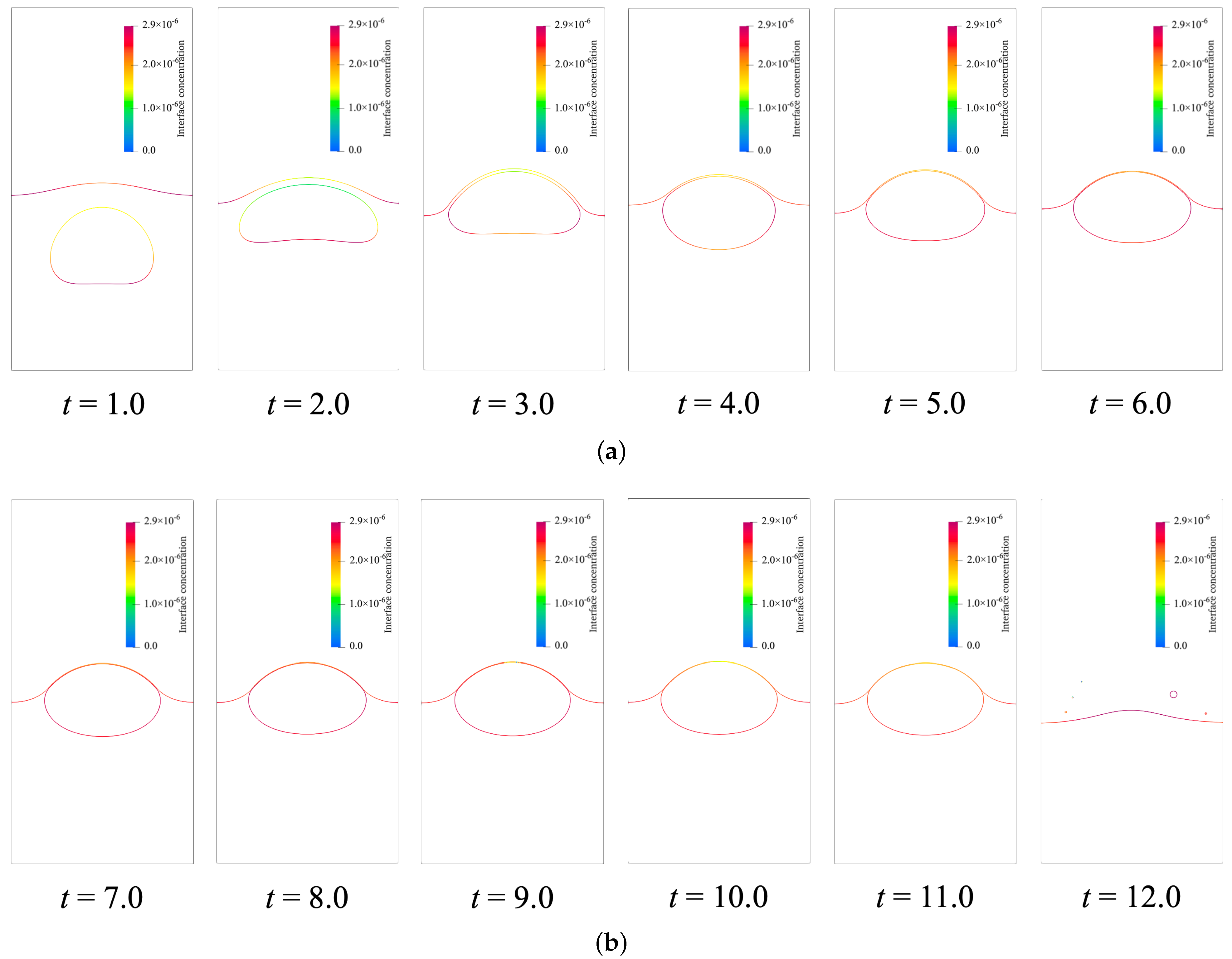
• Section 5.3 describes a simulation of the generation of liquid film by a single bubble rising to a horizontal interface and the rupture process of that liquid film with surfactant transport and the Marangoni effect. The motion of the liquid rim after the rupture of the liquid film observed in the present study’s simulation showed good agreement with the results of previous experiments, which indicates the accuracy of this method and its potential for use in further simulations of multi-scale problems.

The present study’s method can be extended to three dimensions in a straightforward manner. With the Message Passing Interface (MPI), multiple GPUs can be connected and used for a large-scale three-dimensional simulation. The Immersed Boundary Method (IBM) can be implemented for simulations with more complex geometries.

7. Conclusions

In conclusion, the PLIC-HF method was applied to a tree-based interface-adaptive AMR mesh and used to simulate the generation and rupture of thin liquid film. It was used along with the WCS and the evolving pressure projection method as a fluid solver. The mathematical description of the solver and numerical methods are explained in Section 2 and Section 3, respectively. The accuracy and efficiency of the solver were verified by benchmark tests including the single vortex flow and single bubble rising. The processes of liquid film generation and rupture with surfactant transport and the Marangoni effect were directly simulated. The behavior of the liquid rim formed after rupture in the simulation showed good agreement with the results of previous experiments.

References

1. Qiao, C.; Yang, D.; Mao, X.; Xie, L.; Gong, L.; Peng, X.; Peng, Q.; Wang, T.; Zhang, H.; Zeng, H. Recent Advances in Bubble-based Technologies: Underlying Interaction Mechanisms and Applications. Appl. Phys. Rev. 2021, 8, 011315. [Google Scholar] [CrossRef]
2. Abid, S.; Chesters, A. The Drainage and Rupture of Partially-Mobile Films Between Colliding Drops at Constant Approach Velocity. Int. J. Multiph. Flow 1994, 20, 613–629. [Google Scholar] [CrossRef]
3. Mileva, E.; Exerowa, D. Foam Films as Instrumentation in the Study of Amphiphile Self-assembly. Adv. Colloid Interface Sci. 2003, 100–102, 547–562. [Google Scholar] [CrossRef]
4. Chan, D.Y.C.; Klaseboer, E.; Manica, R. Film drainage and coalescence between deformable drops and bubbles. Soft Matter 2011, 7, 2235–2264. [Google Scholar] [CrossRef]
5. Karakashev, S.I.; Manev, E.D. Hydrodynamics of Thin Liquid Films: Retrospective and Perspectives. Adv. Colloid Interface Sci. 2015, 222, 398–412. [Google Scholar] [CrossRef]
6. Liu, B.; Manica, R.; Xu, Z.; Liu, Q. The Boundary Condition at the Air–liquid Interface and Its Effect on Film Drainage Between Colliding Bubbles. Curr. Opin. Colloid Interface Sci. 2020, 50, 101374. [Google Scholar] [CrossRef]
7. Vakarelski, I.U.; Langley, K.R.; Yang, F.; Thoroddsen, S.T. Interferometry and Simulation of the Thin Liquid Film between a Free-Rising Bubble and a Glass Substrate. Langmuir 2022, 38, 2363–2371. [Google Scholar] [CrossRef]
8. Aoki, T.; Hasegawa, Y. A Large-scale Aerodynamics Study on Bicycle Racing. JSAE J. 2020, 74, 18–23. [Google Scholar]
9. Berger, M.J.; Oliger, J. Adaptive Mesh Refinement for Hyperbolic Partial Differential Equations. J. Comput. Phys. 1984, 53, 484–512. [Google Scholar] [CrossRef]
10. Matsushita, S.; Aoki, T. A Computation with Tree-based Amr Method Using Multi-moment Scheme for Conservative Phase-field Equation with a Flux Term. Trans. Jpn. Soc. Comput. Eng. Sci. 2018, 2018, 20180005. [Google Scholar] [CrossRef]
11. Matsushita, S.; Aoki, T. A gas-liquid two-phase flow simulation with interface-adapted amr method. Jpn. J. Multiph. Flow 2019, 33, 96–102. [Google Scholar] [CrossRef] [Green Version]
12. Hirt, C.; Nichols, B. Volume of Fluid (VOF) Method for the Dynamics of Free Boundaries. J. Comput. Phys. 1981, 39, 201–225. [Google Scholar] [CrossRef]
13. Sussman, M.; Smereka, P.; Osher, S. A Level Set Approach for Computing Solutions to Incompressible Two-Phase Flow. J. Comput. Phys. 1994, 114, 146–159. [Google Scholar] [CrossRef]
14. Chiu, P.H.; Lin, Y.T. A Conservative Phase Field Method for Solving Incompressible Two-phase Flows. J. Comput. Phys. 2011, 230, 185–204. [Google Scholar] [CrossRef]
15. Sussman, M.; Puckett, E.G. A Coupled Level Set and Volume-of-Fluid Method for Computing 3D and Axisymmetric Incompressible Two-Phase Flows. J. Comput. Phys. 2000, 162, 301–337. [Google Scholar] [CrossRef]
16. Matsushita, S.; Aoki, T. A Weakly Compressible Scheme with a Diffuse-interface Method for Low Mach Number Wwo-phase Flows. J. Comput. Phys. 2019, 376, 838–862. [Google Scholar] [CrossRef]
17. Sato, K.; Koshimura, S. Fundamental Verification for Tsunami Numerical Simulation Using Lattice Boltzmann Method and PLIC-VOF method. J. JSCE B2 2017, 73, I7–I12. [Google Scholar]
18. Sato, K.; Koshimura, S. Development of Three-dimensional Free Surface Flow Simulation Method by Lattice Boltzmann Method and PLIC-VOF Method. J. JSCE B1 2018, 74, I427–I432. [Google Scholar] [CrossRef]
19. Nahed, J.; Dgheim, J. Estimation Curvature in PLIC-VOF Method for Interface Advection. Heat Mass Transf. 2020, 56, 773–787. [Google Scholar] [CrossRef]
20. Matsushita, S.; Aoki, T. Gas-liquid Wwo-phase Flows Simulation Based on Weakly Compressible Scheme with Interface-adapted AMR Method. J. Comput. Phys. 2021, 445, 110605. [Google Scholar] [CrossRef]
21. Afkhami, S.; Bussmann, M. Height Functions for Applying Contact Angles to 2D VOF Simulations. Int. J. Numer. Methods Fluids 2008, 57, 453–472. [Google Scholar] [CrossRef]
22. López, J.; Zanzi, C.; Gómez, P.; Zamora, R.; Faura, F.; Hernández, J. An Improved Height Function Technique for Computing Interface Curvature from Volume Fractions. Comput. Methods Appl. Mech. Eng. 2009, 198, 2555–2564. [Google Scholar] [CrossRef]
23. Evrard, F.; Denner, F.; van Wachem, B. Height-function Curvature Estimation with Arbitrary Order on Non-uniform Cartesian Grids. J. Comput. Phys. X 2020, 7, 100060. [Google Scholar] [CrossRef]
24. Connington, K.; Lee, T. A review of spurious currents in the lattice Boltzmann method for multiphase flows. J. Mech. Sci. Technol. 2012, 26, 3857–3863. [Google Scholar] [CrossRef]
25. Chen, S.; Doolen, G.D. Lattice Boltzmann Method for Fluid Flows. Annu. Rev. Fluid Mech. 1998, 30, 329–364. [Google Scholar] [CrossRef]
26. Aidun, C.K.; Clausen, J.R. Lattice-Boltzmann method for Complex Flows. Annu. Rev. Fluid Mech. 2010, 42, 439–472. [Google Scholar] [CrossRef]
27. Clausen, J.R. Entropically Damped Form of Artificial Compressibility for Explicit Simulation of Incompressible Flow. Phys. Rev. E 2013, 87, 013309. [Google Scholar] [CrossRef]
28. Toutant, A. General and exact pressure evolution equation. Phys. Lett. A 2017, 381, 3739–3742. [Google Scholar] [CrossRef]
29. Kajzer, A.; Pozorski, J. Application of the Entropically Damped Artificial Compressibility model to direct numerical simulation of turbulent channel flow. Comput. Math. Appl. 2018, 76, 997–1013. [Google Scholar] [CrossRef]
30. Yang, K.; Aoki, T. Weakly Compressible Navier-Stokes Solver Based on Evolving Pressure Projection Method for Two-phase Flow Simulations. J. Comput. Phys. 2021, 431, 110113. [Google Scholar] [CrossRef]
31. Aslam, T.D. A Partial Differential Equation Approach to Multidimensional Extrapolation. J. Comput. Phys. 2004, 193, 349–355. [Google Scholar] [CrossRef]
32. Xu, J.J.; Li, Z.; Lowengrub, J.; Zhao, H. A Level-set Method for Interfacial Flows with Surfactant. J. Comput. Phys. 2006, 212, 590–616. [Google Scholar] [CrossRef] [Green Version]
33. Erik Teigen, K.; Song, P.; Lowengrub, J.; Voigt, A. A diffuse-interface method for two-phase flows with soluble surfactants. J. Comput. Phys. 2011, 230, 375–393. [Google Scholar] [CrossRef]
34. Hayashi, K.; Tomiyama, A. Effects of Surfactant on Terminal Velocity of a Taylor Bubble in a Vertical Pipe. Int. J. Multiph. Flow 2012, 39, 78–87. [Google Scholar] [CrossRef]
35. Weymouth, G.; Yue, D.K.P. Conservative Volume-of-Fluid Method for Free-surface Simulations on Cartesian-grids. J. Comput. Phys. 2010, 229, 2853–2865. [Google Scholar] [CrossRef]
36. Yang, K.; Aoki, T. Scaling of a Conservative Weakly Compressible Solver for Large-scale Two-phase Flow Simulation. In Proceedings of the Parallel and Distributed Computing, Applications and Technologies: 23rd International Conference, PDCAT 2022, Sendai, Japan, 7–9 December 2022; Springer: Berlin/Heidelberg, Germany, 2022. [Google Scholar]
37. Scardovelli, R.; Zaleski, S. Analytical Relations Connecting Linear Interfaces and Volume Fractions in Rectangular Grids. J. Comput. Phys. 2000, 164, 228–237. [Google Scholar] [CrossRef]
38. Aulisa, E.; Manservisi, S.; Scardovelli, R.; Zaleski, S. Interface Reconstruction with Least-squares Fit and Split Advection in Three-dimensional Cartesian Geometry. J. Comput. Phys. 2007, 225, 2301–2319. [Google Scholar] [CrossRef]
39. Osher, S.; Sethian, J.A. Fronts Propagating with Curvature-dependent Speed: Algorithms Based on Hamilton-Jacobi Formulations. J. Comput. Phys. 1988, 79, 12–49. [Google Scholar] [CrossRef]
40. Yokoi, K. A Density-Scaled Continuum Surface Force Model within a Balanced Force Formulation. J. Comput. Phys. 2014, 278, 221–228. [Google Scholar] [CrossRef]
41. Jiang, G.S.; Peng, D. Weighted ENO Schemes for Hamilton–Jacobi Equations. SIAM J. Sci. Comput. 2000, 21, 2126–2143. [Google Scholar] [CrossRef]
42. Harten, A. High Resolution Schemes for Hyperbolic Conservation Laws. J. Comput. Phys. 1997, 135, 260–278. [Google Scholar] [CrossRef]
43. Konstantinidis, E.; Cotronis, Y. Graphics Processing Unit Acceleration of the Red/Black SOR Method. Concurr. Comput. Pract. Exp. 2012, 25, 1107–1120. [Google Scholar] [CrossRef]
44. Fuster, D.; Popinet, S. An All-Mach Method for the Simulation of Bubble Dynamics Problems in the Presence of Surface Tension. J. Comput. Phys. 2018, 374, 752–768. [Google Scholar] [CrossRef]
45. Brackbill, J.; Kothe, D.; Zemach, C. A Continuum Method for Modeling Surface Tension. J. Comput. Phys. 1992, 100, 335–354. [Google Scholar] [CrossRef]
46. Fakhari, A.; Geier, M.; Lee, T. A Mass-conserving Lattice Boltzmann Method with Dynamic Grid Refinement for Immiscible Two-phase Flows. J. Comput. Phys. 2016, 315, 434–457. [Google Scholar] [CrossRef]
47. Yerry, M.A.; Shephard, M.S. Automatic Three-dimensional Mesh Generation by the Modified-octree Technique. Int. J. Numer. Methods Eng. 1984, 20, 1965–1990. [Google Scholar] [CrossRef]
48. Rider, W.J.; Kothe, D.B. Reconstructing Volume Tracking. J. Comput. Phys. 1998, 141, 112–152. [Google Scholar] [CrossRef]
49. Hysing, S.; Turek, S.; Kuzmin, D.; Parolini, N.; Burman, E.; Ganesan, S.; Tobiska, L. Quantitative Benchmark Computations of Two-dimensional Bubble Dynamics. Int. J. Numer. Methods Fluids 2009, 60, 1259–1288. [Google Scholar] [CrossRef]
50. Aland, S.; Voigt, A. Benchmark Computations of Diffuse Interface Models for Two-dimensional Bubble Dynamics. Int. J. Numer. Methods Fluids 2012, 69, 747–761. [Google Scholar] [CrossRef]
51. Klostermann, J.; Schaake, K.; Schwarze, R. Numerical Simulation of a Single Rising Bubble by VOF with Surface Compression. Int. J. Numer. Methods Fluids 2013, 71, 960–982. [Google Scholar] [CrossRef]
52. Turek, S. Efficient Solvers for Incompressible Flow Problems: An Algorithmic and Computational Approache; Springer Science & Business Media: Berlin/Heidelberg, Germany, 1999; Volume 6. [Google Scholar]
53. Parolini, N.; Burman, E. A Finite Element Level Set Method For Viscous Free-surface Flows. In Applied and Industrial Mathematics in Italy; World Scientific Publishing Co. Pte., Ltd.: Chennai, India, 2005; pp. 416–427. [Google Scholar] [CrossRef]
54. John, V.; Matthies, G. MooNMD—A Program Package Based on Mapped Finite Element Methods. Comput. Vis. Sci. 2004, 6, 163–170. [Google Scholar] [CrossRef]
55. Lin, S.Y.; Chang, H.C.; Chen, E.M. The Effect of Bulk Concentration on Surfactant Adsorption Processes: The Shift from Diffusion-Control to Mixed Kinetic-Diffusion Control with Bulk Concentration. J. Chem. Eng. Japan 1996, 29, 634–641. [Google Scholar] [CrossRef]
56. Matsushita, S. Incompressible Gas-Liquid Two-Phase Flow Simulation Based on Weakly Compressible Scheme. Ph.D. Thesis, Tokyo Institute of Technology, Tokyo, Japan, 2020. [Google Scholar]
57. Pandit, A.B.; Davidson, J.F. Hydrodynamics of the rupture of thin liquid films. J. Fluid Mech. 1990, 212, 11–24. [Google Scholar] [CrossRef]
58. Takagi, S. The Effect of Surfactant on the Motion of Rising Bubbles. Nagare J. JSFM 2004, 23, 17–26. [Google Scholar] [CrossRef]
Figure 1. The interface reconstruction and flux calculation used in the Piecewise Linear Interface Calculation (PLIC) method.The region in blue is occupied by heavy fluid and the region in white is occupied by light fluid. The dotted line represents linearized interface in a cell. The black arrow in (a) indicates the normal vector of the interface and the black arrow in (b) indicates the direction of the velocity on that cell face. (a) Interface reconstruction. (b) Flux calculation.
Applsci 13 01955 g001
Figure 2. Dependence of the surface tension coefficient σ on the interface concentration f expressed by the Langmuir state equation. The dotted line indicates the saturation concentration.
Applsci 13 01955 g002
Figure 3. Configuration of the staggered grid system. Vector components are defined at cell faces, and scalars are defined at cell centers.
Applsci 13 01955 g003
Figure 4. Stencil computations of the viscous term where (a) the directions of the derivative and velocity are the same and (b) the directions of the derivative and the velocity are different. (a) Stencil computation where the directions of the derivative and the velocity are the same. (b) Stencil computation where the directions of the derivative and the velocity are different.
Applsci 13 01955 g004
Figure 5. The refinement procedure of a two-dimensional tree-based AMR grid and the corresponding quadtree structure. The purple lines and circles represent leaf nodes.
Applsci 13 01955 g005
Figure 6. The construction of a 8 × 8 stencil without a diagonal halo region in the shared memory. The white cells represent 4 × 4 leaf cells in a leaf node. The light blue cells represent the halo cells of the stencil taken from the X+ and X− directions. The light red cells represent the halo cells of the stencil taken from the Y+ and Y− directions. The light and deep gray cells are not accessed in an 8 × 8 stencil without a diagonal halo region.
Applsci 13 01955 g006
Figure 7. The construction of a 12 × 12 stencil with diagonal halo region in the shared memory. The white cells represent 4 × 4 leaf cells in a leaf node. The light blue cells represent the halo cells of the stencil taken from the X+ and X− directions. The light red cells represent the halo cells of the stencil taken from the Y+ and Y− directions. The light green cells represent the diagonal halo cells of the stencil taken from diagonal directions in a ’neighbor of neighbor’ way.
Applsci 13 01955 g007
Figure 8. Interface deformation in a 2D single vortex. The reconstructed interface is shown as a black line and the AMR grid is shown as a light gray line. The maximum AMR level and finest resolution of (a) and (b) are 2 and 256 × 256 , respectively. The maximum AMR level and finest resolution of (c) and (d) are 3 and 512 × 512 , respectively. (a) t = T 2 , finest resolution 256 × 256 . (b) t = T , finest resolution 256 × 256 . (c) t = T 2 , finest resolution 512 × 512 . (d) t = T , finest resolution 512 × 512 .
Applsci 13 01955 g008
Figure 9. Time evolution of the total cell number on the AMR grid. Maximum AMR refinement level 2 with a finest resolution of 256 × 256 is shown in blue, and maximum AMR level 3 with a finest resolution of 512 × 512 is shown in pink.
Applsci 13 01955 g009
Figure 10. A schematic diagram of the two-dimensional rising bubble problem as a benchmark test. The region in light blue is occupied by heavy fluid and the region in white is occupied by light fluid.
Applsci 13 01955 g010
Figure 11. The shape of the interface in the two-dimensional rising bubble simulation, t = 3 . The red line indicates the results of the AMR grid with a finest resolution of 256 × 512 and the black line indicates the results of the AMR grid with a finest resolution of 512 × 1024 . (a) Case A. (b) Case B.
Applsci 13 01955 g011
Figure 12. The evolution of the center of mass of the bubble compared with the reference results presented by Hysing et al. [49] for the two-dimensional rising bubble problem. The colors of the references indicate the results achieved with TP2D (solid red), FreeLIFE (solid green), and MooNMD (solid blue), as well as the 256 × 512 (solid black) grid and the 512 × 1024 (dashed pink) grid. (a) Case A. (b) Case B.
Applsci 13 01955 g012
Figure 13. The evolution of the rising velocity of the bubble compared with the reference results presented by Hysing et al. [49] for the two-dimensional rising bubble problem. The colors of the references indicate the results achieved with TP2D (solid red), FreeLIFE (solid green), and MooNMD (solid blue), as well as the 256 × 512 (solid black) and 512 × 1024 (dashed pink) grids. (a) Case A. (b) Case B.
Applsci 13 01955 g013
Figure 14. A schematic diagram of liquid film generation and rupture simulation by a single bubble freely rising to an interface. The region presented in light blue is occupied by heavy fluid and the region presented in white is occupied by light fluid.
Applsci 13 01955 g014
Figure 15. Volume fraction profile for the bubble rising to an interface starting from the contaminated state and forming liquid film in surfactant solution with a Langmuir number of L a = 15 , from t = 1.0 to t = 12.0 . The region presented in red contains heavy fluid and the region presented in blue contains light fluid. AMR leaves are shown as light gray lines. (a) Volume fraction profile for the bubble rising to an interface starting from the contaminated state and forming a liquid film in surfactant solution, L a = 15 , from t = 1.0 to t = 6.0 . (b) Volume fraction profile for the bubble rising to an interface starting from the contaminated state and forming liquid film in surfactant solution, L a = 15 , from t = 7.0 to t = 12.0 .
Applsci 13 01955 g015
Figure 16. Volume fraction profile focused on the liquid film area during the rupture process of the liquid film in surfactant solution with a Langmuir number of L a = 15 from t = 11.13 to t = 11.27 with an interval of Δ t = 0.02 . The region presented in red contains heavy fluid, and the region presented in blue contains light fluid. The AMR leaves are shown as light grey lines.
Applsci 13 01955 g016aApplsci 13 01955 g016b
Figure 17. Interface concentration profile for the bubble rising to an interface starting from the contaminated state and forming liquid film in surfactant solution, L a = 15 , from t = 1.0 to t = 12.0 . The color legend ranges from f = 0 to a saturation concentration of f = 2.9 × 10 6 . (a) Interface concentration profile for the bubble rising to an interface starting from the contaminated state and forming liquid film in the surfactant solution, L a = 15 , from t = 1.0 to t = 6.0 . (b) Interface concentration profile for the bubble rising to an interface starting from the contaminated state and forming liquid film in surfactant solution, L a = 15 , from t = 7.0 to t = 12.0 .
Applsci 13 01955 g017
Figure 18. Interface concentration profile focused on the liquid film area during the liquid film rupture process in surfactant solution with a Langmuir number of L a = 15 , from t = 11.13 to t = 11.27 , with an interval of Δ t = 0.02 . The color legend ranges from f = 0 to a saturation concentration of f = 2.9 × 10 6 .
Applsci 13 01955 g018aApplsci 13 01955 g018b