Abstract
The uranium required for power plants is mainly extracted by two methods in roughly equal amounts: quarries (underground and open pit) and in situ leaching (ISL). Uranium mining by in situ leaching is extremely attractive because it is economical and has a minimal impact on the region’s ecology. The effective use of ISL requires, among other things, the accurate assessment of the host rocks’ filtration characteristics. An accurate assessment of the filtration properties of the host rocks allows optimizing the mining process and improving the quality of the ore reserve prediction. At the same time, in Kazakhstan, this calculation is still based on methods that were developed more than 50 years ago and, in some cases, produce inaccurate results. According to our estimates, this method provides a prediction of filtration properties with a determination coefficient = 0.32. This paper describes a method of calculating the filtration coefficient of ore-bearing rocks using machine learning methods. The proposed approach was based on nonlinear regression models providing a 20–75% increase in the accuracy of the filtration coefficient assessment compared with the current methodology. The work used different types of machine learning algorithms based on the gradient boosting technique, bagging technique, feed-forward neural networks, support vector machines, etc. The results of logging, core sampling, and hydrogeological studies obtained during the exploration stage of the Inkai deposit were used as the initial data. All used machine learning models demonstrated significantly better results than the old method. This resulted in improved results compared with previous studies. The LightGBM regressor demonstrated the best result ( = 0.710).
1. Introduction
Intensive development of nuclear energy can be considered one of the means to combat global warming. For example, nuclear power plants in Europe annually avoid the emission of 700 million tons of CO2. Uranium mining is carried out in more than 20 countries, but the main uranium reserves are concentrated in Australia, Kazakhstan, and Canada [1]. According to the World Nuclear Association, in 2018, the largest uranium mining companies produced 86% of the world’s total uranium production [2], of which NAC Kazatomprom JSC accounted for 21%. There are two main extraction methods used: open pit (underground and open-pit) and in situ leaching (ISL). Open pit (accounting for 45.9% of production) is used with a sufficiently high uranium content, ILS (accounting for 48.3% of production) is used with a fairly low uranium content, and the reserves must be located in highly permeable rocks (most often sands). Approximately 5.8% of uranium is mined as a by-product, such as in gold mining [3] (Figure 1).
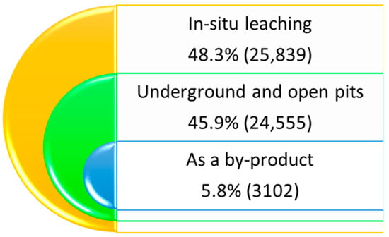
Figure 1.
World uranium mining volumes by mining methods.
ISL is a method of developing of sandstone-type uranium deposits without raising ore to the surface by selectively transferring uranium ions into a productive solution directly in the subsurface using a network of injection and extraction wells. Uranium-bearing ore remains underground, unlike traditional mining methods (mines and quarries). ISL is the most economical and environmentally friendly mining method, widely used in Kazakhstan, Uzbekistan, Canada, and Australia. However, to successfully apply the ISL method, it is necessary to solve the following problems:
- Accurate determination of the lithological composition of the host rocks and the depth of permeable and impermeable strata using geophysical methods;
- Assessment of filtration properties of host rocks, for the correct assessment of recoverable reserves and production planning.
Inaccuracies in solving these problems not only prevent the organization of an optimal production process but often lead to serious financial losses. For example, economic losses from incorrect lithological classification in the deposits of Kazakhstan can be estimated to be approximately USD 1 to 4 million per year [4].
Inaccuracies in assessing the filtration properties of host rocks are caused both by inaccuracies in electrical logging and, to a large extent, by the methodology for determining the lithological composition and filtration properties of rocks. When determining the filtration properties of host rocks in a field, the key point is to determine the relationship between the filtration coefficient Kf, determined as a result of hydrogeological studies at the exploratory drilling stage, and electrical logging data, which are subsequently used to calculate the filtration properties of technological wells. However, the accepted methodology, based on analytical methods, has not changed since the end of the last century [5]. At the same time, the correct determination of Kf is necessary for calculating recoverable reserves, predicting production dynamics, and calculating the optimal number of wells and the distance between them (the diameter of a hexagonal cell or the distance between rows of wells).
One of the promising ways to improve the quality of the filtration properties assessment is the use of artificial intelligence [6], more specifically, machine learning methods [7]. Machine learning is used in problems of stratigraphy [8], geological mapping [9], assessment of the prospects of tungsten deposits [10], composition of iron ore deposits [11], and lithology [12,13,14,15]. The application of ML for lithological classification is considered in [16].
The purpose of the study was to evaluate the possibilities of using machine learning models for calculation based on well log data in sandstone-type uranium deposits.
This study considered the application of machine learning methods to estimate the filtration characteristics of ore-bearing rocks. The method was based on the use of nonlinear regression models and has shown results 20–75% better than calculations using the existing methodology used in Kazakhstan. The proposed method concerns approximately half of the mined uranium in the world.
The work consists of the following sections. The first section briefly provides general information about uranium and its mining methods and the application of machine learning methods in geophysical research.
In the second section, we provide an overview of the current state of research in the field of determining the permeability of geological formations using machine learning.
In the third section, we describe the research method.
In the fourth, we describe the initial data and the results obtained.
In conclusion, the limitations of the method and directions for further research are discussed.
2. Related Works
The permeability of rocks is an important factor influencing the percentage of hydrocarbon recovery, reservoir management, and carbon dioxide sequestration during oil production. During in situ leaching of uranium, rock permeability is the most important factor in deciding whether to install downhole filters and predicting ore recovery.
To solve the problems of permeability predicting, porosity, and other petrophysical properties of rocks in mining, regression models are often used [11], which allow developing more accurate and robust models than traditional empirical, statistical models [17]. Such models have been studied since the 1990s. For example, in Ref. [18], probably for the first time, a multilayer neural network was used to estimate the porosity of rocks. To assess the permeability of rocks, a hybrid algorithm using neural networks (ANNs) was proposed in [19]. An ANN-based regression analysis was used to obtain a set of relationships between the permeability, porosity, and pore size in [20]. ANNs as a non-linear regression method is used to estimate the porosity and permeability of an oil reservoir based on log data [21,22]. A similar problem is considered in [23], where the authors compared ANN, SVM, and fuzzy neural network models. The authors concluded that ANNs can be used to estimate the permeability of a heterogamous carbonate reservoir based on three parameters: the bulk density, the neutron porosity, and a mobility index introduced by the authors with a mean square error of 0.28. In this paper, the authors also used ANNs to estimate the permeability of an oil-bearing reservoir in the Persian Gulf of Egypt and obtained very high values of the coefficient of determination R2 = 96.5%.
In Ref. [24], the porosity of oil reservoirs was studied using ANNs based on seismic sounding data. It was possible to study the petrophysical properties in the interwell space and identify zones of bypass sand channels and leaks that were not visible on the structural maps and attribute slices. The high result of the estimation of the porosity of the oil reservoir based on the SVM model was described in [25], where the correlations between the model estimates and real data exceeded 0.96. The authors of the paper stated that machine learning models worked more accurately than traditional estimation methods [26], reaching RMSE = 0.38 and R2 = 97% for the SVM-based model when processing log data from carbonate reservoirs of southwestern Iran.
Well logs can be considered as a type of images that can be analyzed using deep learning models when there are enough data. For example, to estimate the permeability in the process of oil production in [27], convolutional neural networks (CNNs) were used, which showed an advantage over ANNs. The use of CNNs to predict the properties of subsurface rocks in the process of drilling wells in real time is discussed in [28]. The authors show that the model is able to distinguish between different rock types such as cemented sandstone, unconsolidated sands, and shales. A CNN-based model was proposed in [29] to accompany the technological process of well construction, namely, to assess the integrity of cement in cased wells.
The deep learning model was used to identify the similarity of geological interlayers, and thus, with higher accuracy, allows estimating cross-well correlation [30]. New Zealand and Norway open datasets were used to tune the model. The accuracy of the model was 0.926, which was significantly higher than the base models based on gradient boosting. A similar problem of estimating the interwell space of an oil and gas reservoir is considered in [31], where a three-dimensional CNN is used, which shows better results compared with ANNs.
As shown above, the use of machine learning methods is very popular in the assessment of permeability, porosity, and interwell space in oil fields, where such methods in many cases show good results. However, the situation is different for uranium deposits.
According to the authors, such studies of rock permeability assessment for sandstone-type uranium deposits have not been previously carried out, with the exception of [6]. Meanwhile, uranium mining at such deposits is carried out by the method of in situ leaching, in which the filtration properties of rocks are critically important. The use of regression models to assess the filtration coefficients is a way to improve the accuracy of the calculation of recoverable ore reserves and optimize the mining process.
The range of regression models is quite large. They, like other machine learning models, can be roughly divided into classical and modern ones [6].
Although deep learning provides excellent results in many cases [32], its application is possible, as a rule, in the presence of a large amount of data or in the presence of pre-trained models, using the transfer learning technique [7]. According to the authors, there are no such datasets in the public domain. In this regard, for a comparative assessment of the possibilities of solving the problem of predicting the filtration properties of rocks based on logging data by models of different types, it was decided to use several types of regression models based on support vector algorithms, boosting, bagging, and neural networks.
3. Proposed Method
The methodological scheme of the study included the following steps (Figure 2):
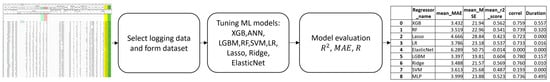
Figure 2.
Methodological scheme of the study.
- Feature selection and dataset generation;
- Training and tuning machine learning models;
- Evaluation of results using standard quality metrics.
3.1. Data Preparation
The methodology currently used provides for the establishment of a relationship between the filtration properties of host rocks and the apparent resistivity measured at the exploration stage. To do this, resistivity logging data are compared with the results of hydrogeological studies of wells and results of granulometric studies [33] (Figure 3).
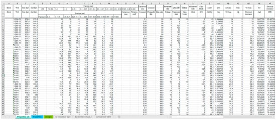
Figure 3.
Data for determining the filtration properties of rocks according to the accepted method.
As a result, a correspondence table is compiled, intermediate values are obtained by interpolation. The disadvantages of the adopted methodology include the fact that it uses data from only one logging method and cannot be used if the recording quality is insufficient, as well as the fact that it uses the average resistivity value within the selected interval, which cannot be accurately determined for intervals with thickness less than 1.5–2 m, since the distance between the measuring electrodes during logging is 1 m. Given the shortcomings of the existing estimation methodology, we proposed a machine learning model that received basic logging data as the input and generated filtration coefficients as the output. Such a model could be trained on data from exploratory wells that have actual (pumped out). The trained model could then be used to calculate of the technological wells.
To form a dataset for training regression models, we used the information collected from the results of research at the exploration stage, shown in Figure 3. Figure 3 shows the boundaries of the well intervals (Start dept, End dept), within which the values of the filtration properties (Kf column) are known; for the same intervals, the granulometric study data, the proportion of clay fraction, and the geochemical (color) and lithological (Lito code) codes are given. In total, there were 3558 intervals in the collected dataset, with a thickness of 0.5 to 2.2 m. However, to build regression models that will be used on production wells, one can use only logging data, as well as the lithological code of rocks, because the rest of the parameters are obtained in the course of laboratory studies and are not available for production wells. For exploratory wells, the standard set of logs included AR (apparent resistivity), SP (spontaneous polarization potential), GL (gamma logging), and inclinometry (determines the angle of inclination of the well). AR and SP were the main methods for lithological classification, with impermeable rocks (clays) corresponding to low AR and high SP values, while highly permeable rocks, vice versa, had high AR and low SP values. The GL and inclinometry were in no way related to the filtration properties; therefore, to build regression models, we chose sections of the AR and SP curves with a length of 0.5 m, as well as the lithological code of the rock, as input parameters.
3.2. Machine Learning Models
As mentioned above, the application of deep learning models could produce a good result. However, the generated dataset is relatively small. The authors also do not know of similar sets of initial data of a significant volume or pre-trained models of deep neural networks that solve the problem of calculating the permeability of rocks in uranium deposits, which would allow using the transfer learning technique to tune them. Therefore, the use of deep learning models was considered inappropriate. In the process of the computational experiments, the authors used several types of models: models based on gradient boosting [34] and bagging technique, feed-forward neural networks [16], support vector machines, and, as a reference point (baseline) for comparative analysis, classical regression algorithms (Table 1).

Table 1.
Machine learning models.
The variety of algorithm types provides a broad search for the appropriate type of models. Looking ahead, we note that the ensemble learning methods, and more precisely the gradient boosting models, generally showed the best result.
To assess the quality of regression models, the following accuracy indicators were used [47]:
Coefficient of determination (R2);
Mean square error (mean squared error—MSE);
Mean absolute error (mean absolute error—MAE);
Correlation coefficient (R).
The quality measures used to evaluate the regression models are listed in Table 2.
Table 2.
Evaluation metrics of regression models.
To perform computational experiments, a software system was developed in Python using the numpy, sklearn, matplotlib, cv2, alive_progress, pickle, and tensorflow libraries, which enable the reading and preparing of the initial data, forming a data frame, and applying machine learning models. The computational experiments were performed on a Dell XPS 15 9500 computer equipped with 32 GB of RAM, an Intel(R) Core(TM) i7-10750H processor, and an Nvidia GeForce GTX 1650 Ti discrete graphics card. All equipment is manufactured in China.
4. Data and Results
In total, there were 3558 intervals in the collected dataset, with a thickness of 0.5 to 2.2 m. As input parameters, sections of the AR and SP curves with a thickness of 0.5 m, recorded with a step of 0.1 m, as well as the lithological code of the rock, determined by the experts, were used. During the experiments, nine regression models were tested: XGB, RF, Lasso, Linear regression, Elastic Net, LGBM, Ridge, SVM, and ANN (hidden_layer_size = 91) on all combinations of input parameters (AR, SP, AR + SP, AR + lithocode, SP + lithocode, and AR + SP + lithocode). The XGB, RF, and LGBM models did not require data normalization (more precisely, normalization of input parameters can degrade the performance of these models), while other models worked better with normalized data. The normalization was performed using the standard function MinMaxScaler() included in the sklearn package. The results of the experiments are shown in Table 3.
Table 3.
Assessments of the performance of the models trained on the exploration wells.
In the last row, for comparison, the results of the calculations according to the currently accepted method are given. It can be seen that the best set of input data was the combination of AR + lithocode, while the use of SP significantly worsened the accuracy of the models. This was probably due to the low quality of the PS curve recording. Since the recorded potential depended on the difference between the salinity of groundwater and the drilling fluid, for contrast and differentiable recording of SP, it was necessary to strictly adhere to the requirements for the preparation of the drilling fluid, which was often not observed in practice. Because the size of the dataset was small, the training time for all algorithms was less than 1 s.
The LGBM regressor showed the best results when using (AR, Litho code) as the input parameters ( = 0.710). At the same time, when we could use only a part of the input parameters, other regression models could also be used. For example, a linear regression model performed well when we could only use SP, and we did not know the lithological code ( = 0.415). In cases where we could only use the AR values, the best result again showed LGBM ( = 0.604). In addition, linear regression (LR) showed a stable good result. The currently used methodology showed significantly worse results compared with machine learning models ( = 0.32). A comparison of the data calculated with accepted methodology with actual data showed that the RMSE was 13.89 and the linear correlation value was 0.584. This low accuracy was probably due to the fact that 0.5 m intervals were used for comparison, while the accepted methodology was designed for intervals with thickness more than 2 m.
5. Conclusions
For efficient and safe uranium mining using the ISL method, it was necessary to determine as accurately as possible the lithological composition of the host rocks and the depth of permeable and impermeable strata, as well as the filtration properties of the host rocks. The necessary dependencies could be determined by comparing data from hydrogeological studies carried out at the exploration stage with logging data. In Kazakhstan, a method for determining the filtration properties was used, developed more than 50 years ago, which often produced incorrect results. Inaccuracies in the assessment of the filtration properties of host rocks led to the incorrect assessment of recoverable reserves and poor production planning. The currently accepted technique was based on the dependence of Kf on the average value of the AR within the boundaries of the selected lithological layer and had the following disadvantages:
- Only the AR curve data were used; if the AR data were poorly recorded, the results would be unreliable.
- When interpreting data from acidified blocks, where the properties of rocks were distorted by the action of acid, the values of the AR turned out to be underestimated, and therefore, the calculation of the filtration properties was not correct.
- Since a downhole tool with a distance between electrodes of 1 m was used to record AR logs in the fields of Kazakhstan, it was possible to reliably measure the average resistivity value only for lithological layers with a thickness of more than 2 m. Therefore, the adopted technique was not suitable for thin intervals (<2 m).
To overcome the shortcomings of the existing approach, we proposed a method for calculating the filtration coefficient based on the use of regression models [48]. The proposed model received electric logging data as an input and the calculated filtration coefficient as an output.
Thanks to a wider range of regression models, it was possible to improve the previously obtained result.
The LGBM regression model with AR and LC as the input variables demonstrated the best results ( = 0.710, R = 0.845).
At the same time, the proposed method had the following limitations:
- It was not applicable to fields where exploration had been carried out for a long time, and not all the necessary data were available.
- The learning process depended on the lithological code set by the expert, which could be wrong, especially in the case of acidified blocks.
In this regard, directions for further research are the following:
- Exploring the possibility of transferring the trained model to similar fields for which there are no data required for training;
- Improving the reliability of determining the lithological code of the rock during lithological classification;
- Automatic identification of zones of technological acidification by the characteristic distortion of the AR curve.
Also, as one of the future research directions, it is suggested to use the construction of a forecasting model based on Fuzzy Decision Trees [49].
Author Contributions
Conceptualization, R.M., Y.K. and E.Z.; methodology, R.M.; software, A.S.; validation, Y.K., E.Z., V.L. and A.S.; formal analysis, R.M. and N.Y.; investigation, K.A., V.L., E.M. and Y.K.; resources, Y.K., R.M. and E.M.; data curation K.A., A.S. and V.L.; writing—original draft preparation, R.M., Y.K. and E.Z.; writing—review and editing, Y.K. and N.Y.; visualization, Y.K.; supervision, R.M.; project administration, Y.K.; funding acquisition, N.Y. All authors have read and agreed to the published version of the manuscript.
Funding
This research was funded by the Committee of Science of the Ministry of Science and Higher Education of the Republic of Kazakhstan (Grant No. AP14869110 “Improving the accuracy of solving problems of interpretation of geophysical well research data on uranium deposits using machine learning methods”) and was partially supported by the Slovak Research and Development Agency, Slovakia, under the grant “Risk assessment of environmental disturbance using Earth observation data” (reg.no. SK-UA-21-0037).
Institutional Review Board Statement
Not applicable.
Informed Consent Statement
Not applicable.
Data Availability Statement
Not applicable.
Acknowledgments
The authors express their sincere gratitude to Viktors Gopejenko and Sergey Stankevich, who actively supported this work.
Conflicts of Interest
The authors declare no conflict of interest.
References
- Uranium Reserves, Which Countries Have the Largest Reserves? Available online: https://www.energy.com (accessed on 28 June 2023).
- World Nuclear Association. “Recent Uranium Production”, The Nuclear Fuel Report: Expanded Summary—Global Scenarios for Demand and Supply Availability 2019–2040. 2020. Available online: https://world-nuclear.org/getmedia/b488c502-baf9-4142-8d12-42bab97593c3/nuclear-fuel-report-2019-expanded-summary-final.pdf.aspx (accessed on 30 June 2023).
- International Energy Agency (IEA). Key World Energy Statistics. Also Available on Smartphones and Tablets. 2016. Available online: https://www.ourenergypolicy.org/wp-content/uploads/2016/09/KeyWorld2016.pdf (accessed on 30 June 2023).
- Mukhamediev, R.I.; Kuchin, Y.I.; Yakunin, K.O.; Mukhamedieva, E.L.; Kostarev, S.V. Preliminary results of the assessment of lithological classifiers for uranium deposits of the infiltration type. Cloud Sci. 2020, 7, 258–272. [Google Scholar]
- Guidelines for Determining the Coefficient of Filtration of Water-Bearing Rocks by Experimental Pumping, Energoizdat. 1981. Available online: https://www.geokniga.org/books/17383 (accessed on 15 June 2023).
- Mukhamediev, R.I.; Popova, Y.; Kuchin, Y.; Zaitseva, E.; Kalimoldayev, A.; Symagulov, A.; Levashenko, V.; Abdoldina, F.; Gopejenko, V.; Yakunin, K.; et al. Review of Artificial Intelligence and Machine Learning Technologies: Classification, Restrictions, Opportunities and Challenges. Mathematics 2022, 10, 2552. [Google Scholar]
- Mukhamediev, R.I.; Symagulov, A.; Kuchin, Y.; Yakunin, K.; Yelis, M. From classical machine learning to deep neural networks: A simplified scientometric review. Appl. Sci. 2021, 11, 5541. [Google Scholar] [CrossRef]
- Merembayev, T.; Yunussov, R.; Yedilkhan, A. Machine learning algorithms for stratigraphy classification on uranium deposits. Procedia Comput. Sci. 2019, 150, 46–52. [Google Scholar] [CrossRef]
- Cracknell, M.J. Machine Learning for Geological Mapping: Algorithms and Applications. Ph.D. Thesis, University of Tasmania, Hobart, TAS, Australia, 2014. [Google Scholar]
- Sun, T.; Li, H.; Wu, K.; Chen, F.; Zhu, Z.; Hu, Z. Data-driven predictive modeling of mineral prospectivity using machine learning and deep learning methods: A case study from southern Jiangxi Province, China. Minerals 2020, 10, 102. [Google Scholar] [CrossRef]
- Dogan, A.; Birant, D.; Kut, A. Multi-target regression for quality prediction in a mining process. In Proceedings of the 2019 4th International Conference on Computer Science and Engineering (UBMK), Samsun, Turkey, 11–15 September 2019; pp. 639–644. [Google Scholar]
- Deng, C.; Pan, H.; Fang, S.; Konate, A.A.; Qin, R. Support vector machine as an alternative method for lithology classification of crystalline rocks. J. Geophys. Eng. 2017, 14, 341–349. [Google Scholar] [CrossRef]
- Kumar, C.; Chatterjee, S.; Oommen, T.; Guha, A. Automated lithological mapping by integrating spectral enhancement techniques and machine learning algorithms using AVIRIS-NG hyperspectral data in Gold-bearing granite-greenstone rocks in Hutti, India. Int. J. Appl. Earth Obs. Geoinf. 2020, 86, 102006. [Google Scholar]
- Cracknell, M.J.; Reading, A.M. Geological mapping using remote sensing data: A comparison of five machine learning algorithms, their response to variations in the spatial distribution of training data and the use of explicit spatial information. Comput. Geosci. 2014, 63, 22–33. [Google Scholar]
- Harris, J.R.; Grunsky, E.C. Predictive lithological mapping of Canada’s North using Random Forest classification applied to geophysical and geochemical data. Comput. Geosci. 2015, 80, 9–25. [Google Scholar] [CrossRef]
- Kuchin, Y.I.; Mukhamediev, R.I.; Yakunin, K.O. One method of generating synthetic data to assess the upper limit of machine learning algorithms performance. Cogent Eng. 2020, 7, 1718821. [Google Scholar] [CrossRef]
- Khan, H.; Srivastav, A.; Kumar Mishra, A.; Anh Tran, T. Machine learning methods for estimating permeability of a reservoir International. J. Syst. Assur. Eng. Manag. 2022, 13, 2118–2131. [Google Scholar]
- Wong, P.M.; Henderson, D.J.; Brooks, L.J. Reservoir permeability determination from well log data using artificial neural networks: An example from the Ravva field, offshore India. In Proceedings of the Petroleum Development under Challenging Environments (with Special Emphasis on Gas), Kuala Lumpur, Malaysia, 14–16 April 1997; pp. 149–155. [Google Scholar]
- Matinkia, M.; Hashami, R.; Mehrad, M.; Hajsaeedi, M.R.; Velayati, A. Prediction of permeability from well logs using a new hybrid machine learning algorithm. Petroleum 2023, 9, 108–123. [Google Scholar] [CrossRef]
- Rezaee, M.R.; Jafari, A.; Kazemzadeh, E. Relationships between permeability, porosity and pore throat size in carbonate rocks using regression analysis and neural networks. J. Geophys. Eng. 2006, 3, 370–376. [Google Scholar] [CrossRef]
- Lim, J.S. Reservoir properties determination using fuzzy logic and neural networks from well data in offshore Korea. J. Pet. Sci. Eng. 2005, 49, 182–192. [Google Scholar] [CrossRef]
- Antoniuk, V.; Bezrodna, I.; Petrokushyn, O. Multiple regressions and ann techniques to predict permeability from pore structure for terrigenous reservoirs, west-shebelynska area Monitoring. Eur. Assoc. Geosci. Eng. 2019, 2019, 1–5. [Google Scholar]
- Elkatatny, S.; Mahmoud, M.; Tariq, Z.; Abdulraheem, A. New insights into the prediction of heterogeneous carbonate reservoir permeability from well logs using artificial intelligence network. Neural Comput. Appl. 2018, 30, 2673–2683. [Google Scholar] [CrossRef]
- Fajana, A.O.; Ayuk, M.A.; Enikanselu, P.A. Application of multilayer perceptron neural network and seismic multi-attribute transforms in reservoir characterization of Pennay field, Niger Delta. J. Pet. Explor. Prod. Technol. 2019, 9, 31–49. [Google Scholar] [CrossRef]
- Ahmadi, M.A.; Ahmadi, M.R.; Hosseini, S.M.; Ebadi, M. Connectionist model predicts the porosity and permeabil-ity of petroleum reservoirs by means of petro-physical logs: Application of artificial intelligence. J. Pet. Sci. Eng. 2014, 123, 183–200. [Google Scholar] [CrossRef]
- Talebkeikhah, M.; Sadeghtabaghi, Z.; Shabani, M. A comparison of machine learning approaches for prediction of permeability using well log data in the hydrocarbon reservoirs. J. Hum. Earth Future 2021, 2, 82–99. [Google Scholar] [CrossRef]
- Zhong, Z.; Carr, T.R.; Wu, X.; Wang, G. Application of a convolutional neural network in permeability prediction: A case study in the Jacksonburg-Stringtown oil field, West Virginia, USA. Geophysics 2019, 84, 363–373. [Google Scholar] [CrossRef]
- Kanfar, R.; Shaikh, O.; Yousefzadeh, M.; Mukerji, T. Real-time well log prediction from drilling data using deep learning. In Proceedings of the International Petroleum Technology Conference, Dhahran, Saudi Arabia, 13 January 2020. [Google Scholar]
- Viggen, E.M.; Merciu, I.A.; Løvstakken, L.; Måsøy, S.E. Automatic interpretation of cement evaluation logs from cased boreholes using supervised deep neural networks. J. Pet. Sci. Eng. 2020, 195, 107539. [Google Scholar] [CrossRef]
- Romanenkova, E.; Rogulina, A.; Shakirov, A.; Stulov, N.; Zaytsev, A.; Ismailova, L.; Kovalev, D.; Katterbauer, K.; AlShehri, A. Similarity learning for wells based on logging data. J. Pet. Sci. Eng. 2022, 215, 110690. [Google Scholar] [CrossRef]
- Du, S.; Wang, R.; Wei, C.; Wang, Y.; Zhou, Y.; Wang, J.; Song, H. The connectivity evaluation among wells in reservoir utilizing machine learning methods. IEEE Access 2020, 8, 47209–47219. [Google Scholar] [CrossRef]
- Sudakov, O.; Burnaev, E.; Koroteev, D. Driving digital rock towards machine learning: Predicting permeability with gradient boosting and deep neural networks. Comput. Geosci. 2019, 127, 91–98. [Google Scholar] [CrossRef]
- Physical Basis for Determining the Lithological and Filtration Properties of Rocks of the Productive Horizon. 2018. Available online: https://ozlib.com/832945/tehnika/fizicheskie_osnovy_metoda (accessed on 10 July 2023).
- Friedman, J.H. Greedy function approximation: A gradient boosting machine. Ann. Stat. 2001, 29, 1189–1232. [Google Scholar] [CrossRef]
- Chen, T.; Guestrin, C. Xgboost: A scalable tree boosting system. In Proceedings of the 22nd ACM Sigkdd International Conference on Knowledge Discovery and Data Mining, New York, NY, USA, 13 August 2016; pp. 785–794. [Google Scholar]
- Ke, G.; Meng, Q.; Finley, T.; Wang, T.; Chen, W.; Ma, W.; Liu, T.Y. Lightgbm: A highly efficient gradient boosting decision tree. Adv. Neural Inf. Process. Syst. 2017, 30, 3149–3157. [Google Scholar]
- Al Daoud, E. Comparison between XGBoost, LightGBM and CatBoost using a home credit dataset. Int. J. Comput. Inf. Eng. 2019, 13, 6–10. [Google Scholar]
- Bentéjac, C.; Csörgő, A.; Martínez-Muñoz, G. A comparative analysis of gradient boosting algorithms. Artif. Intell. Rev. 2021, 54, 1937–1967. [Google Scholar] [CrossRef]
- Breiman, L. Random Forests. Mach. Learn. 2001, 45, 5–32. [Google Scholar] [CrossRef]
- Cortes, C.; Vapnik, V. Support-vector networks. Mach. Learn. 1995, 20, 273–297. [Google Scholar] [CrossRef]
- Hornik, K.; Stinchcombe, M.; White, H. Multilayer feedforward networks are universal approximators. Neural Netw. 1989, 2, 359–366. [Google Scholar] [CrossRef]
- Galushkin, A.I. Theory of Neural Networks; Hotline-Telecom; Springer: Berlin/Heidelberg, Germany, 2010; p. 496. [Google Scholar]
- Yu, H.F.; Huang, F.L.; Lin, C.J. Dual coordinate descent methods for logistic regression and maximum entropy models. Mach. Learn. 2011, 85, 41–75. [Google Scholar] [CrossRef]
- Santosa, F.; Symes, W. Linear inversion of band-limited reflection seismograms. SIAM J. Sci. Stat. Comput. 1986, 7, 1307–1330. [Google Scholar] [CrossRef]
- Tikhonov, A.N.; Goncharsky, A.V.; Stepanov, V.V.; Yagola, A.G.; Tikhonov, A.N.; Goncharsky, A.V.; Yagola, A.G. Numerical Methods for the Approximate Solution of Ill-Posed Problems on Compact Sets; Springer: Dordrecht, The Netherlands, 1995; pp. 65–79. [Google Scholar]
- Hoerl, A.E.; Kennard, R.W. Ridge regression: Applications to nonorthogonal problems. Technometrics 1970, 12, 69–82. [Google Scholar] [CrossRef]
- Zou, H.; Hastie, T. Regularization and variable selection via the elastic net. J. R. Stat. Soc. Ser. B Stat. Methodol. 2005, 67, 301–320. [Google Scholar] [CrossRef]
- Mukhamediev, R.I.; Kuchin, Y.; Amirgaliyev, Y.; Yunicheva, N.; Muhamedijeva, E. Estimation of Filtration Properties of Host Rocks in Sandstone-Type Uranium Deposits Using Machine Learning Methods. IEEE Access 2022, 10, 18855–18872. [Google Scholar] [CrossRef]
- Zaitseva, E.; Levashenko, V. Construction of a reliability structure function based on uncertain data. IEEE Trans. Reliab. 2016, 65, 1710–1723. [Google Scholar] [CrossRef]
Disclaimer/Publisher’s Note: The statements, opinions and data contained in all publications are solely those of the individual author(s) and contributor(s) and not of MDPI and/or the editor(s). MDPI and/or the editor(s) disclaim responsibility for any injury to people or property resulting from any ideas, methods, instructions or products referred to in the content. |
© 2023 by the authors. Licensee MDPI, Basel, Switzerland. This article is an open access article distributed under the terms and conditions of the Creative Commons Attribution (CC BY) license (https://creativecommons.org/licenses/by/4.0/).