Abstract
Airborne bathymetric LiDAR (ABL) acquires waveform data with better accuracy and resolution and greater user control over data processing than discrete returns. The ABL waveform is a mixture of reflections from the water surface and bottom, water column backscattering, and noise, and it can be separated into individual components through waveform decomposition. Because the point density and positional accuracy of the point cloud are dependent on waveform decomposition, an effective decomposition technique is required to improve ABL measurement. In this study, a new progressive waveform decomposition technique based on Gaussian mixture models was proposed for universal applicability to various types of ABL waveforms and to maximize the observation of seafloor points. The proposed progressive Gaussian decomposition (PGD) estimates potential peaks that are not detected during the initial peak detection and progressively decomposes the waveform until the Gaussian mixture model sufficiently represents the individual waveforms. Its performance is improved by utilizing a termination criterion based on the time difference between the originally detected and estimated peaks of the approximated model. The PGD can be universally applied to various waveforms regardless of water depth or underwater environment. To evaluate the proposed approach, it was applied to the waveform data acquired from the Seahawk sensor developed in Korea. In validating the PGD through comparative evaluation with the conventional Gaussian decomposition method, the root mean square error was found to decrease by approximately 70%. In terms of point cloud extractability, the PGD extracted 14–18% more seafloor points than the Seahawk’s data processing software.
1. Introduction
Bathymetry, the measurement of underwater topography, is a prerequisite for many hydrological applications, such as flood forecast and prevention, maritime ecosystem monitoring, and sustainable development of wetlands [1,2]. Traditional bathymetry approaches based on field measurements have achieved precise results, but they are laborious, time-consuming, and infeasible in unnavigable areas [3]. Accordingly, airborne bathymetric LiDAR (ABL) has been introduced as a promising alternative tool because of its fast and efficient data acquisition capability, acceptable accuracy, and high spatial density [4,5].
With the rapid advance in LiDAR hardware, most current ABL systems adopt full-waveform systems, which acquire the returned signals with a very short sample interval of less than 1 ns. The entire time history of the reflected signal can be restored, and valuable information regarding not only the target position but also its properties can be extracted from the waveform data. The full-waveform LiDAR system yields more detailed and accurate three-dimensional (3D) maps [6,7,8] and value-added information, such as seafloor roughness [9], suspended sediment concentrations [10], or water turbidity [11]. However, the use of ABL waveform data is limited in practice due to difficulties associated with their analysis. Consequently, the potential of ABL waveform data has not been fully exploited.
The LiDAR waveform comprises multiple returns from various targets and non-negligible noise. The simple and traditional method for measuring the target position involves using the waveform to detect peak positions induced by returns from targets. Several methods have been applied, including the center of gravity, local maximum, zero-crossing of the second derivative, and averaged square difference function [12,13]. However, peak detection methods cannot be utilized to derive valuable properties, such as the amplitude and width of the return pulses, by focusing on the positions of the peaks. Measuring the position and radiation characteristics of each target requires a waveform decomposition process that can separate a continuous signal into individual return signals [14,15].
Waveform decomposition divides the returned waveform signals from different targets into multiple individual parameterized components. Accordingly, suitable parameterized functions for each returned waveform should be assumed to distinguish the meaningful components accurately. A Gaussian model is generally utilized for waveform decomposition [9,16]. The approximated parameters (e.g., amplitude, center, and width) of each decomposed Gaussian component are related to the target’s physical properties and can be used as waveform features for further applications such as point classification [17,18,19] and land–water discrimination [20,21]. Conventional Gaussian decomposition (CGD) approximates individual waveforms with Gaussian models of the number of previously detected peaks [22]. The CGD technique exhibits stable decomposition performance when applied to topographic LiDAR data in urban or forest areas where multiple return pulses are separate and have prominent peaks [23,24]. However, it may not be suitable for asymmetric ABL waveforms with a peak left shift due to attenuation of the return pulse energy [25,26], which can lead to point omissions for seafloor objects [18].
Different mathematical models for ABL waveform decomposition have been designed for different sensor and surveying environments. In most models, the ABL waveform is assumed to be decomposed into three distinguishable contributions: returns from the water surface, water column, and bottom (or seafloor). Returns from the water surface or bottom are generally approximated based on the Gaussian or Weibull model [14,15,26]. On the contrary, triangular [14], quadrilateral [15], and improved quadrilateral models [26], among others, have been used for modeling the returns from the water column considering the asymmetry due to the exponentially attenuated amplitude. Other studies have proposed mathematical models considering the water depth because it affects the shape of the returned signals. A depth-adaptive decomposition method was proposed by adopting two individual mathematical models according to the water depth [27]. One was an empirical function based on the calibration waveform for shallow water, and the other was an improved quadrilateral function with a second polynomial for deep water. A decomposition method for very shallow water (< 2 m) was also developed based on boxcar and exponential functions [28]. Waveform decomposition based on the separated functions for the three contributions can be efficient because the meaningful signals (i.e., the returns of the water surface and bottom for bathymetry) are simultaneously defined; therefore, bathymetric maps can be immediately generated. However, they are only applicable to typical waveforms in the ideal case (e.g., low-turbidity water without unexpected obstacles such as marine organisms or foam). In practice, the ABL waveform may not include returns from the bottom due to significant attenuation by the water column or include prominent returns from unexpected objects in the water, such as fish or seaweed. Multiple returns from the bottom due to seafloor unevenness may also be included. Furthermore, waveform decomposition techniques that rely on these fixed models encounter challenges when applied to further applications because of their limited ability to extract waveform features from each individual decomposed component. Hence, considering the varying characteristics of coastal and inland water, a flexible Gaussian decomposition method that does not fix the specified model for each contribution or limit the number of mathematical models may be desirable.
A few methods employing a flexible number of Gaussian models for approximating returned ABL waveforms have been developed. One of the early studies on waveform data processing involved decomposing the ABL waveform into multiple Gaussian models and using the parameters of one of the extracted Gaussian distributions to estimate the seafloor roughness [9]. Another noteworthy study [25] proposed the Gaussian half-wavelength progressive decomposition (GHPD) method. The GHPD progressively decomposes a waveform using half-wavelength Gaussian functions based on the time sequence of received echo signals, aiming to reduce the problems of unreasonable decomposition and position shift of reflected pulse peaks caused by echo superposition. This approach is effective in decomposing ABL waveforms of various shapes and improves bathymetry performance, especially in shallow water. Other flexible Gaussian decomposition approaches were mainly investigated for application to topographic LiDAR data. Progressive waveform decomposition (PWD) was proposed to detect and fit distinct return components successively via peak detection [29]. PWD shares similarities with GHPD in that it utilizes a sequential subtraction strategy but progressively decomposes a waveform, starting with the maximum peak, in the order of signal intensity rather than time. Although the sequential subtracting decomposition techniques are fast and flexible, they may inherently involve the risk of overestimating components decomposed earlier and overlooking ambiguous peaks. Linearly approximated iterative Gaussian decomposition (LAIGD) linearly estimates the degree of overlap between adjacent Gaussian components and performs Gaussian modeling according to the deformation impact rank by overlap [30]. Another flexible Gaussian decomposition method utilizes a genetic algorithm to estimate overlapping peaks that are not detected in the initial peak detection [31]. These flexible Gaussian decomposition approaches offer a general applicability regardless of waveform types or characteristics, facilitating the extraction of physical properties (waveform features) from each decomposed component. However, the techniques generally rely on the residual between the waveform and approximate model as a termination criterion for progressive processes. This can potentially lead to the omission of weak reflections (such as those of deep seafloors) in ABL waveforms.
In this study, we aimed to propose a novel flexible Gaussian decomposition approach that can be generally applied to practical ABL waveform data. The primary objectives of the method are as follows:
- Decompose ABL waveforms of various types and shapes;
- Improve the extractability of seafloor points by detecting elusive seafloor signals.
The proposed approach decomposes an ABL waveform to multiple Gaussian models by progressively estimating the potential components that are not sensed during peak detection. The decomposition performance is improved by utilizing a termination criterion based on the time difference between the originally detected and estimated peaks as well as the residuals between the original waveform and the approximated model. The approach was demonstrated through experiments with the waveform data acquired by Seahawk, an ABL system [32].
The remainder of this paper is organized as follows. In Section 2, the test site and data employed in the experiments are described. Section 3 provides the theoretical foundation and details of the proposed approach. Experimental results and evaluations are presented in Section 4. Section 5 presents the discussion, and Section 6 concludes with the summary and final remarks.
2. Materials
The proposed approach was tested on two Seahawk waveform datasets acquired at different water depths and seafloor terrains on the eastern and southern coasts of South Korea.
2.1. Seahawk System
Seahawk was developed by Geostory Inc. since 2014 to monitor wetlands and coasts in Korea. The system can measure co-registered green and NIR laser beams using a holographic optical element [32]. It was designed to measure more than one point on a area at up to 35 m depth in clear water at a flight altitude of 400 m. The ABL point cloud is generated from raw observation data using its own software, namely the Lidar BAthymetry SyStem—Data processing (LBASSD); the data processing algorithms are not disclosed. Since its first successful flight on July 1, 2018, Seahawk has been used for bathymetric measurements of coastal zones, focusing on coastal erosion monitoring in South Korea. Details of the Seahawk system are listed in Table 1.

Table 1.
Specifications of Seahawk system.
The Seahawk system digitizes the received analog signal at 1.6 Giga samples per second; thus, the time bin resolution of the waveform is 0.625 ns. The Seahawk individual waveform is recorded in 2400 bins at 16 bits (0–65,536 digital number (DN)) per sample. The system assumes a 35 m underwater arrival time of 160 ns when the laser transmission angle is 20°. Therefore, considering the round-trip propagation time, 1 bin (0.625 ns) of the waveform corresponds to a depth difference of approximately 0.068 m.
2.2. Test Data
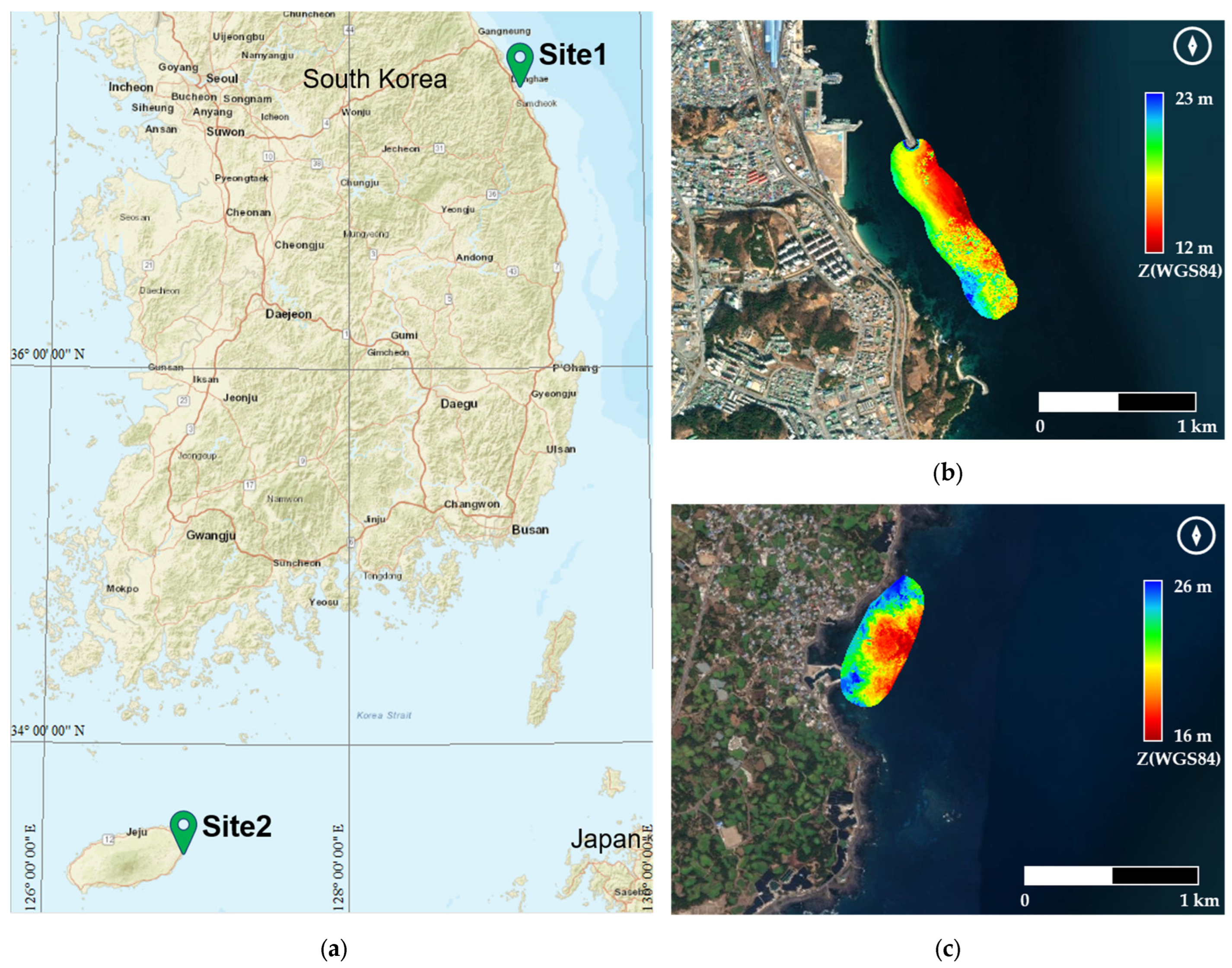
To verify the validity of the proposed approach and its bathymetric performance, we selected two waveform datasets where the water depth at the site is within the observation range of the Seahawk system (maximum depth < 35 m), and seafloor observations for some local areas are missing. Figure 1 shows the locations and seafloor height (WGS84 Ellipsoid) ranges of the two test sites. The first test data were acquired from the eastern coast of Donghae-Si, Gangwon-Do, South Korea. The eastern coast of the Korean Peninsula is ridge-shaped with a monotonous coastline and steep slope where the seafloor rises to land, and the tidal difference is small. The coast has a predominantly sandy substrate and is subject to coastal erosion influenced by waves [33]. The dataset consists of 286,720 waveforms for a 381,392 m2 area with water depth ranging from 5 to 16 m in water depth (Table 2). The second test site is located offshore of the southeastern coast of Jeju Island, which is an uplifted terrain created by volcanic activity. It includes various volcanic coastal terrains, such as coastal cliffs and rock formations, on the southern coast [34]. The dataset was acquired from a rocky shore mainly comprising basalt with an uneven seafloor topography. It includes 143,360 waveforms for a 215,152 m2 area ranging from 0 to 9.5 m in water depth (Table 2).

Figure 1.
Test sites of Seahawk: (a) locations of the test sites; (b) test site 1 on eastern coast of Donghae, Korea; (c) test site 2 on southeastern coast of Jeju Island, Korea.
Table 2.
Summary of the test datasets.
To objectively evaluate the experimental results, the echo-sounding data acquired at a similar time with the test data were utilized as the ground truth. Multibeam echo-sounder (MBES) data are generally used as ground truth for bathymetry; however, a ship-mounted MBES system usually measures water depths greater than 4 m. Accordingly, single-beam echo-sounder (SBES) data were used in test site 2, which has shallow water. The MBES data for test site 1, acquired in November 2021, were surveyed approximately four months before the Seahawk data were obtained. The SBES data for test site 2 were measured in June 2022, representing a three-month gap from the date the Seahawk data were acquired.
3. Methods
The green laser beam used for ABL traverses the water surface and propagates in the water column until it reaches the bottom (Figure 2). The amplitude is rapidly attenuated by absorption, scattering, and refraction. If the beam is not entirely attenuated while traveling through the air–water interface, the backscatter signal reaches back to the receiver, revealing the water surface and bottom positions through peaks in the waveform [35]. A typical ABL waveform is composed of the water surface return, water column backscatter return, bottom return, and noise [10]. Each component is separated through waveform decomposition, and points from the decomposed components are registered.
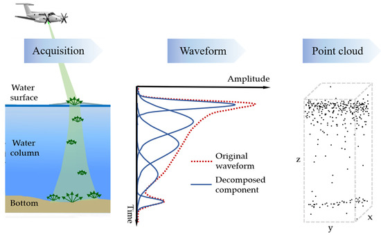
Figure 2.
Data generation in airborne bathymetric LiDAR system.
A LiDAR waveform is a convolution between a transmitted laser pulse and a surface scattering function, both of which are generally considered to follow a Gaussian model. Waveforms received through multipaths can be represented as Gaussian mixture models [24], as in Equation (1), where , , , and denote the number of Gaussian models, amplitude, center position, and standard deviation of the ith Gaussian model, respectively. Because the parameters of Gaussian mixture models have physical meanings related to the position, intensity, and properties of the signal, the characteristics of individual signals can be analyzed through the parameters. To approximate the waveform to the nonlinear model, iteration optimization, such as the Levenberg–Marquardt technique, is performed. In this process, initial values for each parameter (, , , and ) are required. In particular, it is important to select initial values for the iterative operation to finally converge to a global rather than a local solution.
Generally, the Gaussian decomposition technique approximates a waveform to the Gaussian mixture models using peak parameters (amplitude, center, and width) extracted via peak detection as initial values. This CGD relies on peak detection results and is suitable for waveforms in which individual return pulses are detected as separate peaks. However, the ABL waveform is continuously scattered during underwater signal propagation, and multiple Gaussian return signals are densely overlapped, resulting in a signal tilted to the left. It is challenging to separate the overlapped underwater backscattering components by CGD, which consequently imposes limitations on precisely decomposing the water surface and bottom returns.
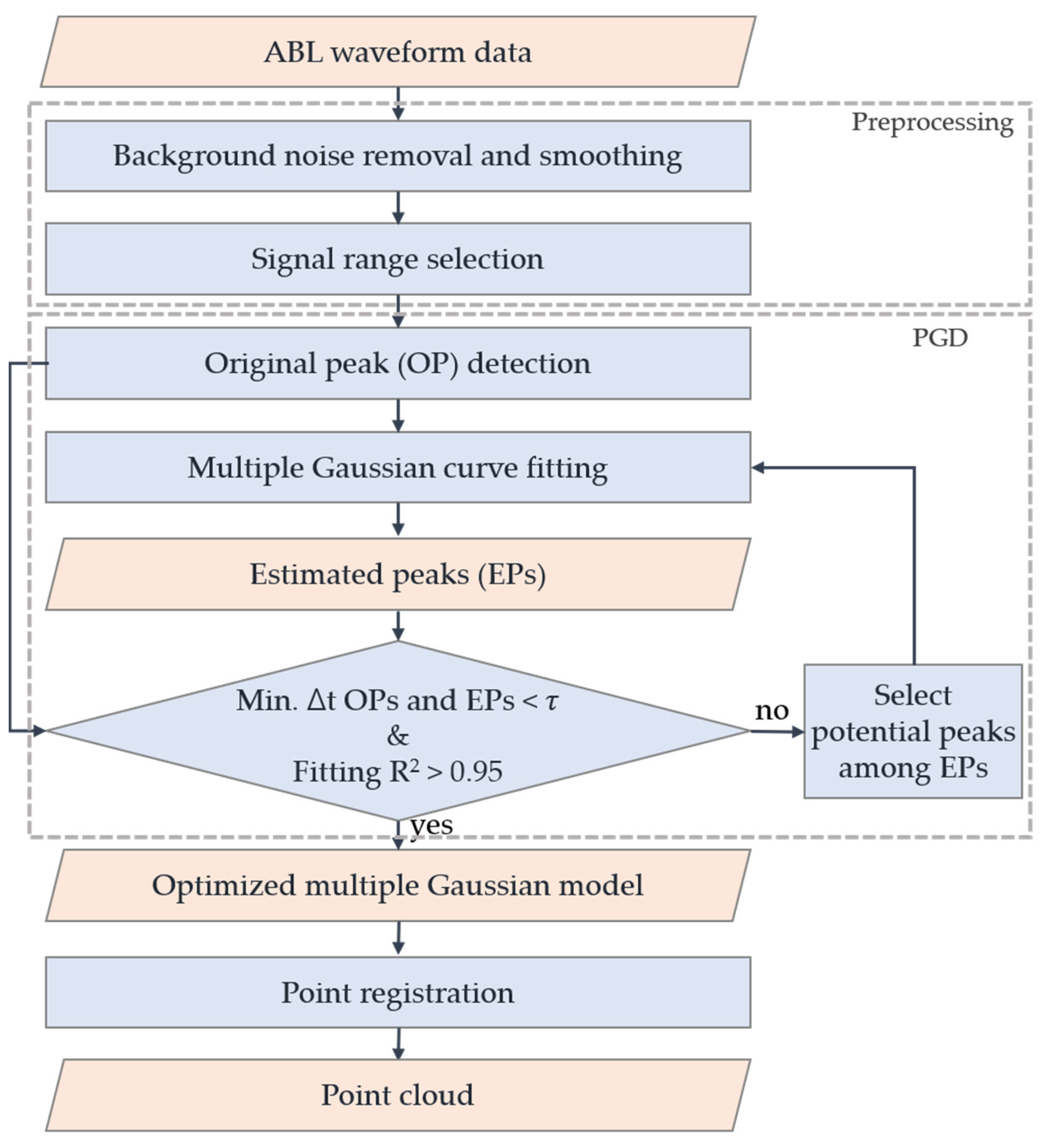
In this study, a progressive Gaussian decomposition (PGD) method is proposed to effectively decompose the ABL waveform data. The proposed approach gradually decomposes a waveform by estimating the overlapping peaks that are undetected during the initial peak detection (Figure 3). The PGD method uses the detected peaks as the first initial value but is not bound by them. It repeats multiple Gaussian curve fitting, progressively estimating potential peaks (PPs) until the desired criteria are achieved. Denoising and signal range selection are performed as preprocessing in the proposed approach. The detailed process is as follows.
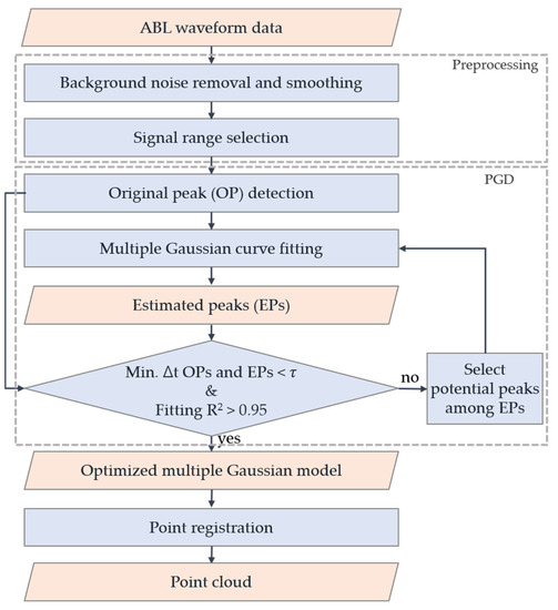
Figure 3.
Workflow of progressive Gaussian decomposition (PGD) process.
3.1. Noise Removal and Signal Range Selection
The waveform includes background noise and random noise caused by environmental and systematic factors. Background noise is long-term, low-frequency noise that is mainly related to solar radiation and detector dark current. In contrast, random noise is short-term, high-frequency noise that is mainly caused by random fluctuations inherent in the acquisition [36]. Systematic background noise tends to be uniformly distributed throughout the duration of the signal and is traditionally removed by applying a threshold [23,36]. However, because the amount of background noise can slightly vary for each waveform, applying a constant threshold to all waveforms acquired in a single flight may not be appropriate. Accordingly, a threshold value for each waveform, such as the mean value at the non-signal range [29] or a wavelet adaptive threshold [37], is commonly used. Because the main contribution to DN in the non-signal range occupying most of the waveform is background noise, we assumed that the most frequently recorded DN value in each waveform would be reflecting the background noise. The background noise is removed by subtracting the mode of an individual waveform, as follows:
where and are the original waveform and the waveform with background noise removed, respectively. Low-pass filtering techniques are mainly used to remove random noise [38,39]. In this study, the waveform is smoothed through Gaussian filtering to remove random noise:
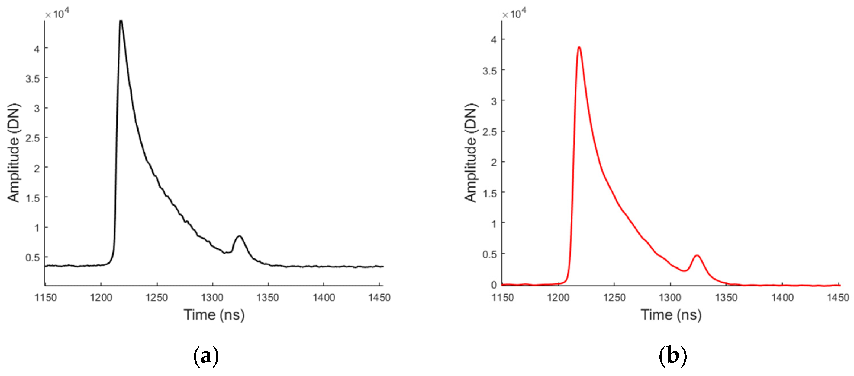
where is the Gaussian filtered value at time , indicates the number of waveform samples, and is the standard deviation of the Gaussian distribution. The larger is, the more smoothing is performed, which may be effective in removing noise, but a return signal with low intensity may be ignored. In this study, was 1. Figure 4 presents an example of a waveform signal before and after noise removal.

Figure 4.
Examples of noise removal: (a) original bathymetric waveform; (b) waveform after background and random noise removal.
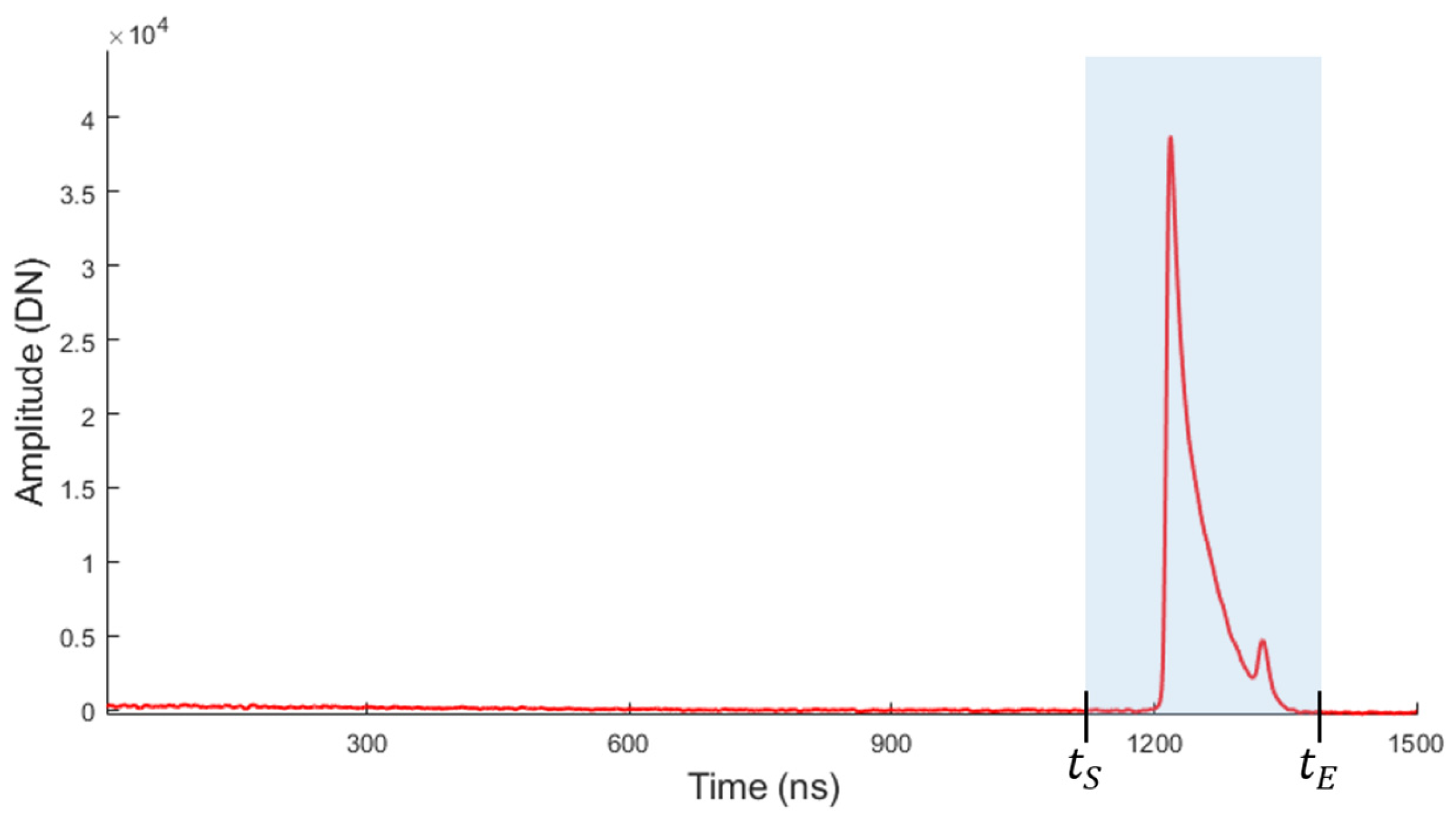
In a waveform with thousands of samples, the range over which the signal reflected from the actual targets is recorded occupies a short part of all the recording samples [25,27]. The range depends on the flight altitude, transmission angle, topographic elevation, and water depth. Therefore, if the actual signal range can be determined, the waveform processing can be more efficient. Moreover, the generation of noise-induced outlier points can be avoided. In the criterion suggested in [40], signal range was detected if the waveform was at least triple the standard deviation of noise for a 5 ns duration. Another study [27] assumed the last 10% of the waveform as the non-signal range and estimated the mean and standard deviation of the amplitude of this interval as the noise level. The interval with an amplitude greater than the mean plus three standard deviations was selected as the signal range. The Seahawk system records 2400 waveform samples over a period of 1.5 µs, during which no reflection signal is returned for the first 0.11 µs. In this study, the first 0.1 µs (160 bins) of the Seahawk waveform was considered as the non-signal range, and the signal range was selected based on the standard deviation in this period. The start and end points of the signal range, and , respectively, are determined as follows (Figure 5).
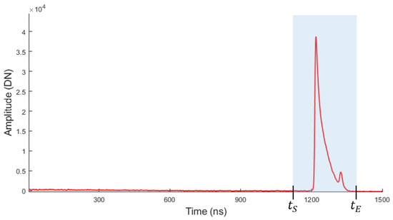
Figure 5.
Example of signal range selection.
As given by Equation (4), , making the start of the water surface return with a distinct intensity increase, is selected as the point where the amplitude increases by more than . To avoid the failure of detecting the bottom peak, which may have a relatively low intensity, was selected as the point where the amplitude decreased to or less, as shown in Equation (5).
3.2. Progressive Gaussian Decomposition
The proposed PGD adopts an iterative approach to estimate the most appropriate number of Gaussian models for decomposing the individual waveform. It initiates an iteration according to the number of detectable peaks within the selected signal range, and the number of Gaussian models is gradually increased. The original peaks (OPs) were detected using findpeaks, a MATLAB peak detection function [41]. The amplitude, center, and width (, and , respectively) of each peak are used as the initial values for the first iteration. In this study, multiple Gaussian curve fitting was implemented using fit, a MATLAB curve fitting toolbox function [42]. Consequently, the number of initially approximated Gaussian components is equal to the number of OPs, and the estimated peaks (EPs) of each component are derived. The fitness of an approximated Gaussian mixture model is typically evaluated using residual-based measures, such as the error ratio [31]. In this study, R2 is used to measure the residual between the original waveform () and approximated Gaussian mixture model (:
However, the evaluation using residual measures may ignore and miss components corresponding to relatively small amplitude peaks (e.g., deep bottom return). In view of this, another criterion is suggested in addition to the residual measure. If the Gaussian curve fitting is successfully performed, the OPs and their corresponding EPs should be located in similar positions. Therefore, we devised a new criterion, i.e., the time difference () between each OP and corresponding (closest) EP, as follows:
where represents the number of estimated Gaussian components, is the number of OPs, and represents the number of iterations. If all values are less than the temporal threshold (τ) and R2 > 0.95, the decomposition is deemed successful, and the process is terminated. Otherwise, if any is greater than τ or R2 ≦ 0.95, the decomposition is considered incomplete, and further iteration is performed. Because Gaussian curve fitting is dependent on the initial value, deciding the initial value to apply in the next iteration in addition to OPs is critical. If the EPs located far from the OPs are estimated, it means that the more dominant Gaussian components than the components corresponding to the OPs have not been undetected in the peak detection. To refer the undetected component to the initial values, the most distant EP from the OPs, i.e., the EP least related to the OPs, is selected as the PP and added as an initial value to the next iteration. In the rth iteration, r EPs are selected as PPs according to the order of those temporally farthest from the OPs. The time difference () between an EP and the closest OP serves as the criterion for selecting the PP and is as follows:
The PGD process can be expressed as the following steps:
Step ⅰ. ;
Step ⅱ. ; Gaussian curve fitting with
Step ⅲ.
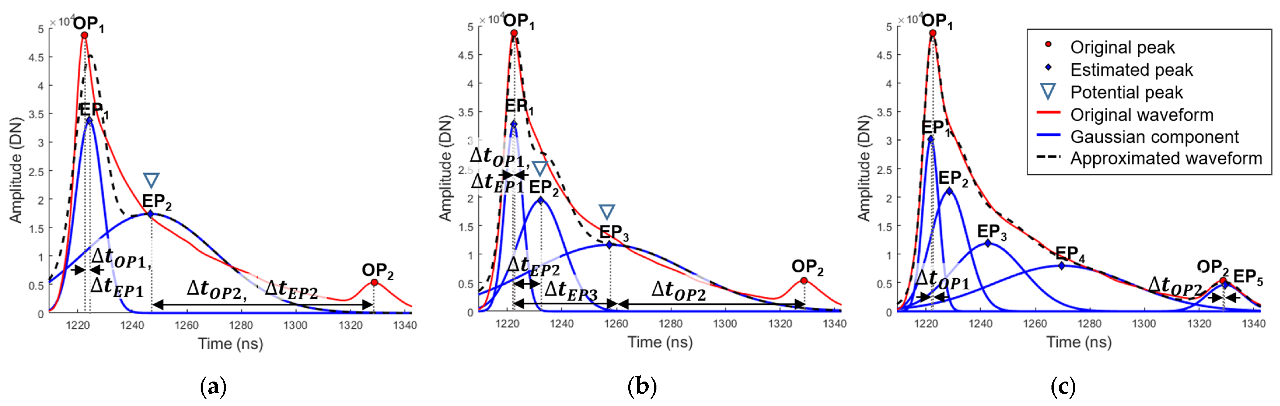
Figure 6 presents the steps involved in the iterative PGD process. Two OPs ( and ), which represent the water surface and bottom returns, respectively, are extracted through peak detection. The first Gaussian curve fitting is performed using these two peaks as initial values (Figure 6a). The peaks of the estimated two Gaussian components ( and ) are located on the water surface and water column backscatter returns, respectively. Thus, the between and the nearest EP () is significantly large. Because the termination criteria are not satisfied, with the largest is selected as the PP. Then, is added as a new initial value along with and for the next iteration. Figure 6b shows the second fitting result decomposed into three Gaussian components using three initial values. Because is smaller than the previous fitting but still greater than , further iteration is required. For the third fitting, two EPs ( and ) are selected as PPs in the order of increasing , and the next fitting is performed with four initial values (, , , and ). Accordingly, the number of PPs is gradually increased according to the number of iterations. The PPs are not accumulated; instead, they are newly selected among the recent EPs at each iteration. As shown in Figure 6c, Gaussian curve fitting was iterated until all converged below . Eventually, the final Gaussian mixture models were determined.
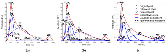
Figure 6.
Iterative steps of PGD: (a) first iteration with original peaks (OPs); (b) second iteration with the OPs and potential peaks; (c) final PGD result.
The threshold, τ, represents the allowable temporal error on the waveform time bins in the Gaussian curve fitting, which is determined according to the required fitness or depth precision and sensor systematic characteristics. Too small τ values can cause overfitting and increase computational time, whereas too large values can reduce depth precision. In this study, the value of τ was set to 5 bins through a preliminary experiment. In a Seahawk system with a waveform sampling interval (1 bin) of 0.625 ns, assuming a transmission angle of 20° and a flight altitude of 400 m and considering a water surface refraction angle of 14.9°, 5 bins can be regarded as a depth difference of approximately 0.34 m.
4. Results
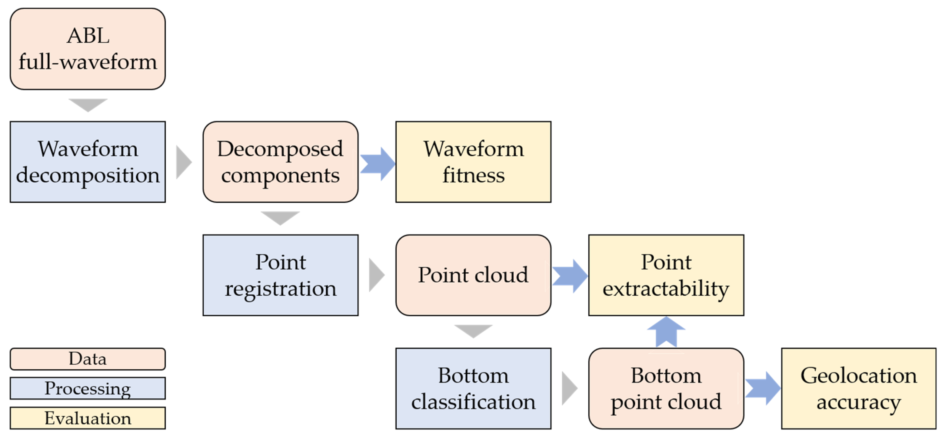
To validate the effectiveness of the proposed PGD approach, its performance is quantitatively and qualitatively evaluated using the Seahawk waveform dataset, as illustrated in Figure 7. To evaluate its applicability to diverse and complex waveforms, the fitness of PGD is compared with that of CGD, which simply approximates the Gaussian mixture model based on peak detection. In addition, to evaluate the improvement in the seafloor measurement performance of the proposed approach, the extractability and geolocation accuracy of bottom points are assessed after point registration. The bottom point extractability (number of points) of the point cloud generated by PGD is compared with that of the point cloud generated by the LBASSD (Seahawk’s processing software). Lastly, the geolocation accuracies of the bottom points extracted using PGD and LBASSD are compared by referring to echo-sounding data.
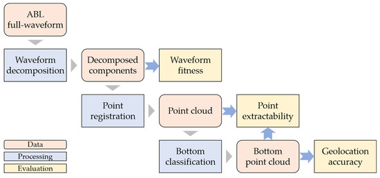
Figure 7.
Evaluation steps of waveform decomposition.
4.1. Fitness Evaluation
To assess the decomposition performance of the proposed PGD on diverse waveform types, quantitative evaluation and qualitative analysis are implemented, the results are compared with those of CGD. Several indicators that measure fitness were calculated for quantitative assessment. The root mean squared error (RMSE) and R2 are used to measure the error between the original waveform () and Gaussian mixture model ( approximated through waveform decomposition. In addition, the structural similarity index map (SSIM) [43] is referenced to evaluate the structural fitness:
where indicates the number of waveform samples, is the covariance, and and are the variables for adjusting the weak denominator. The general constant parameters are and , and the dynamic range of the signal is [43].
The smaller the RMSE value and the closer R2 and SSIM are to 1, the higher the fitness. The mean and standard deviation of the fitness indicators are listed in Table 3. For a more intuitive evaluation of the RMSE magnitude, it has been expressed as normalized RMSE (nRMSE) scaled to a waveform amplitude range (65,536 DN). In both test datasets, the PGD was found to approximate the ABL waveforms better than the CGD. In test site 1, PGD exhibited better fitness than CGD in terms of error (nRMSE = 0.179), approximation (R2 = 0.978), and structural similarity (SSIM = 0.907). The approximation error decreased by approximately 72% in nRMSE, and R2 and SSIM improved by 0.269 and 0.372, respectively. In test site 2, the fitness of PGD was indicated by nRMSE = 0.0260, R2 = 0.980, and SSIM = 0.901. In the foregoing, nRMSE decreased by approximately 66%, and R2 and SSIM improved by 0.172 and 0.206, respectively, compared with those of the CGD results.
Table 3.
Fitness evaluation results of conventional Gaussian decomposition (CGD) and progressive Gaussian decomposition (PGD).
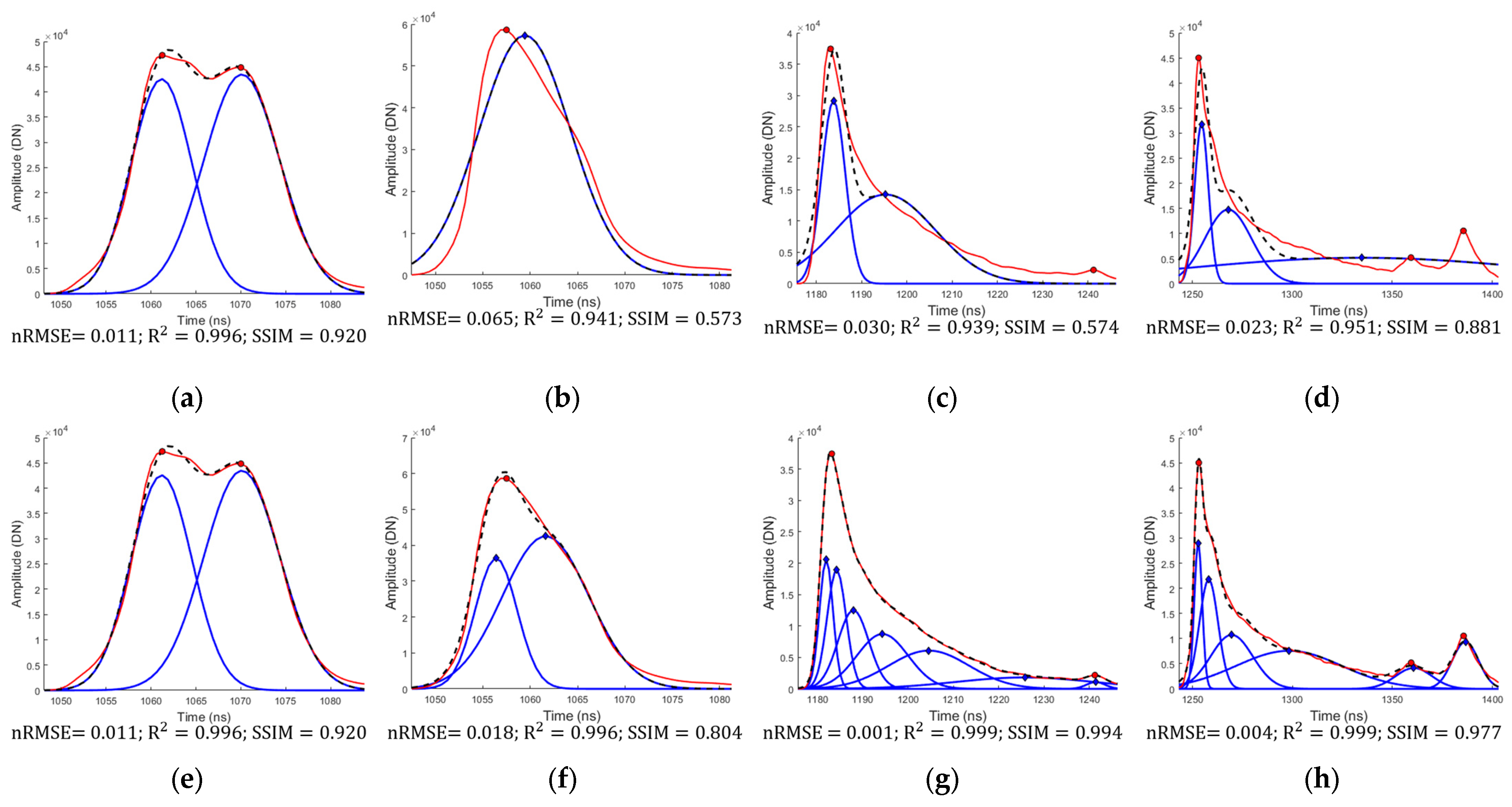
To analyze how the proposed approach is applied to various ABL waveforms, experiments were performed on waveform types with different peak numbers and shapes, and the results were compared. The curves shown on the upper part of Figure 8 are the decomposition results obtained via CGD, and those on the lower part are the decomposition results obtained via the proposed PGD. Figure 8a,e show the waveform with similar intensities of water surface and bottom returns in shallow water, and each return component has its own peak. When each return is detected, both CGD and PGD successfully decompose the waveform into the same components. However, as shown in Figure 8b,f, in shallower waters, the water surface and bottom components closely overlap; hence, the bottom return peak may not be detected. Consequently, the bottom point could not be extracted by CGD, but PGD can measure even a very shallow bottom by decomposing the potential components. The bottom return signal shown in Figure 8c,g is very weakly detected compared with the water surface return, and two OPs are present. Although the bottom return was detected during the initial peak detection, the bottom component was not decomposed by CGD due to its weak intensity (Figure 8c). However, because PGD gradually estimates potential components until the initially detected peak is decomposed into separate components, the bottom return is successfully measured (Figure 8g). Figure 8d,h show a complex waveform type with multiple peaks resulting from underwater objects such as fish and corals or rugged seafloor topography. The underwater peaks and bottom returns were not properly decomposed in the CGD results (Figure 8d), but PGD effectively decomposed multiple peaks by estimating three additional Gaussian components (Figure 8h). These examples confirm that the proposed PGD successfully decomposes different types of waveforms.

Figure 8.
Comparison of waveform decomposition results between CGD and PGD techniques: (a–d) CGD results; (e–h) PGD results.
4.2. Point Extractability Evaluation
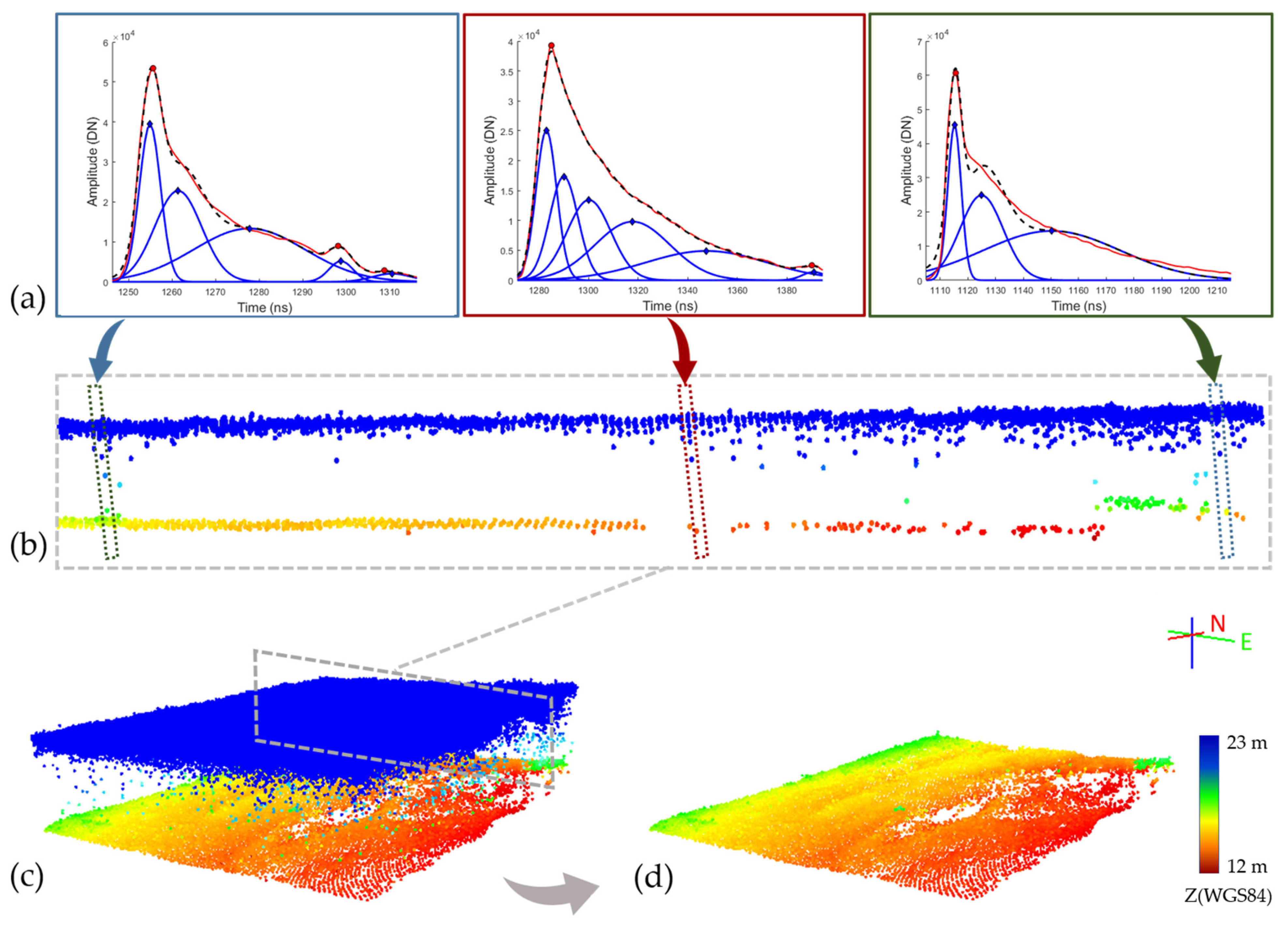
To identify the quantitative improvement in bathymetry performance achieved using the PGD method, decomposed components were registered to coordinated points and subsequently compared with a point cloud generated utilizing LBASSD software. Because the bathymetry performance depends on seafloor observation, bottom points were extracted by manually classifying each point cloud generated by PGD and LBASSD. Figure 9 depicts the process of generating and classifying points from different types of waveforms decomposed by PGD.
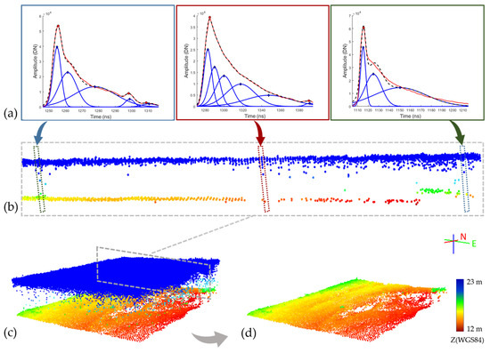
Figure 9.
Point cloud of test site 1 generated by PGD: (a) examples of decomposed waveforms; (b) cross-section of point cloud; (c) regional 3D point cloud; (d) bottom point cloud.
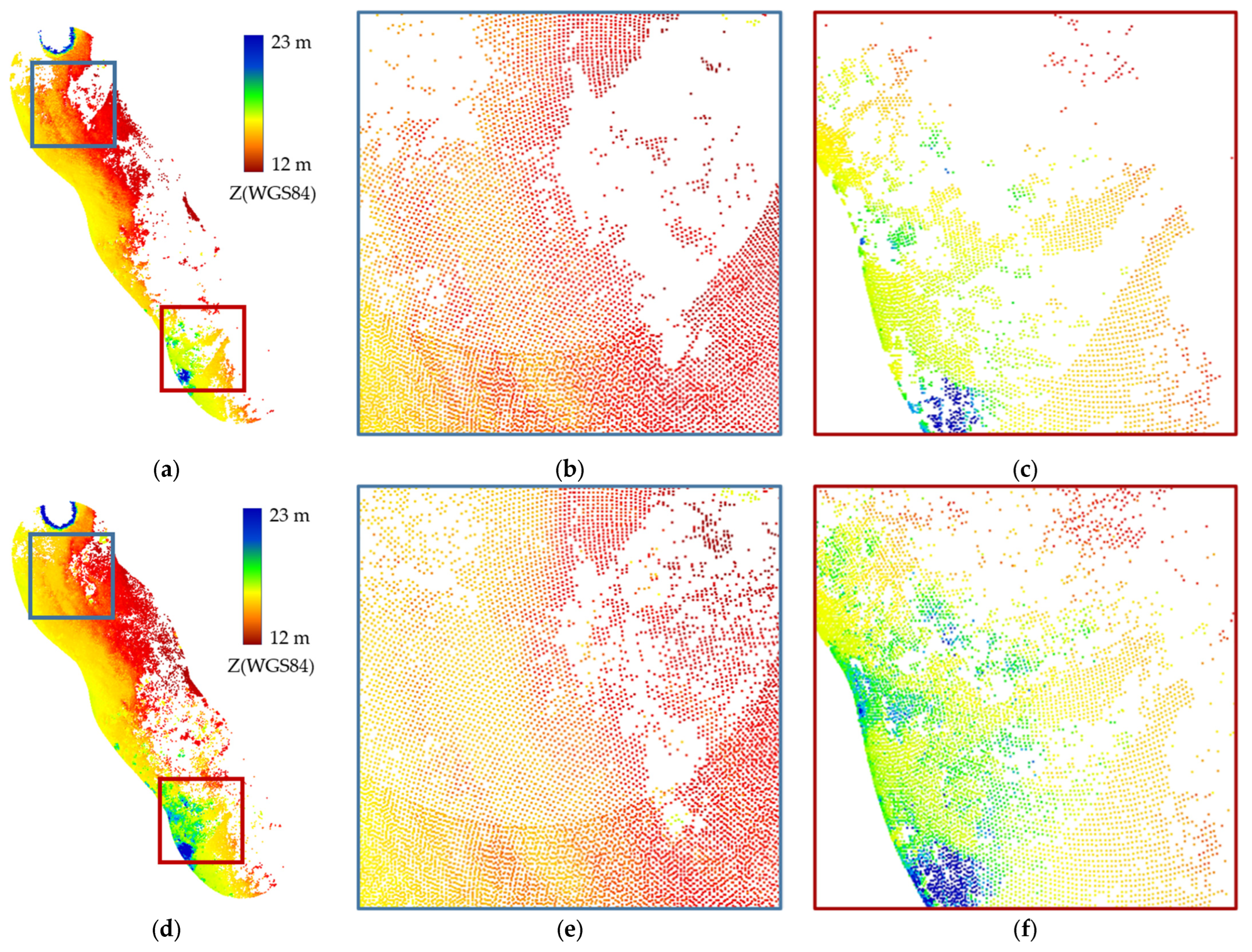
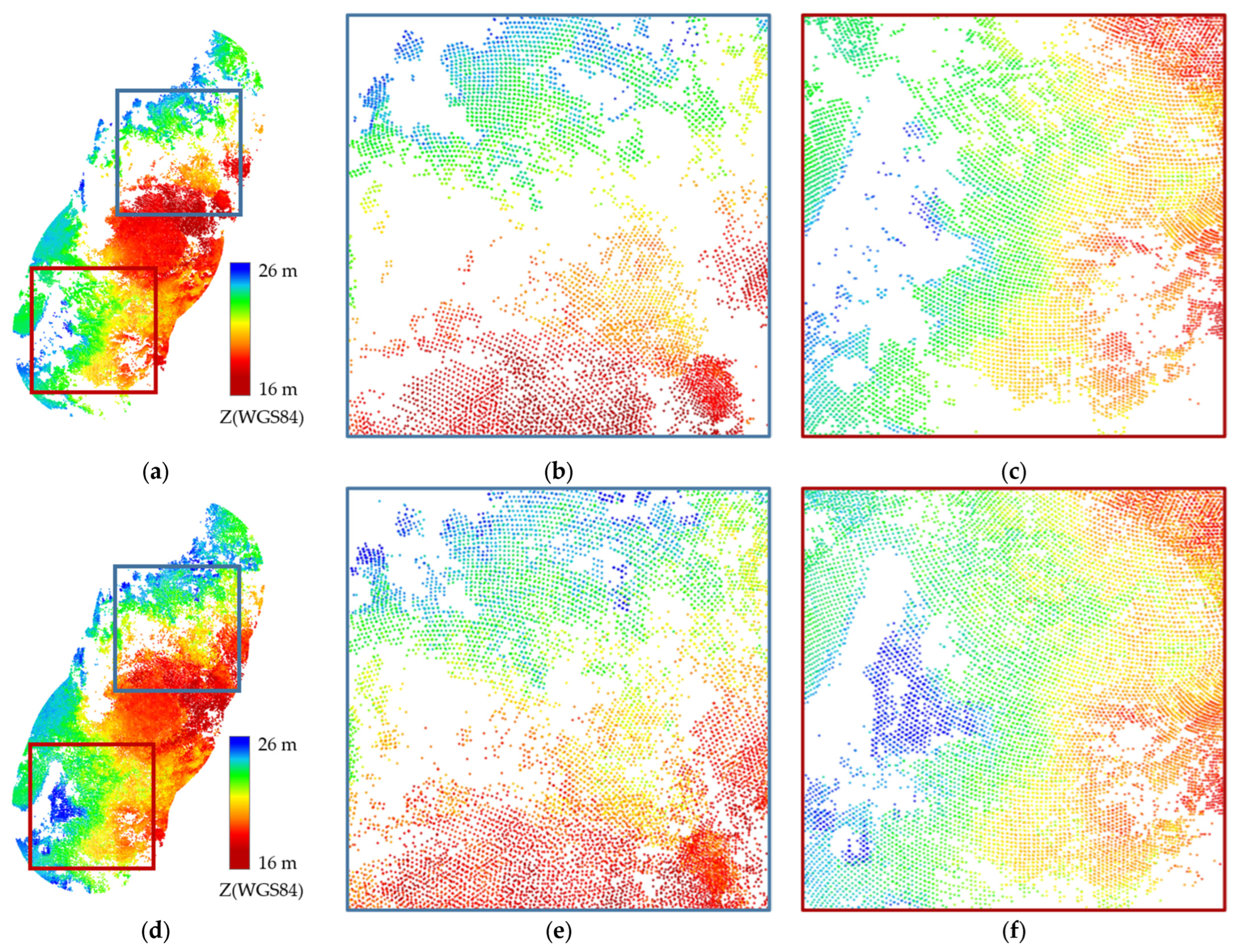
The number of points and point densities were compared for the entire point cloud and point clouds classified as bottom (Table 4). In both test sites, the point cloud extracted through PGD exhibited significantly improved performance compared to the point cloud generated by the LBASSD software. In test site 1, the total number of points (979,283) and point density (2568 pts/m2) generated through PGD were 127% higher than those from the LBASSD results (number of points: 430,376; point density: 1.128 pts/m2). Because the PGD decomposed the water column part into separate components, the total number of points considerably increased. Regarding the bottom points, which are more significant than the total number of points, the number of points (76,336) and point density (0.200 pts/m2) increased by 18%. In test site 2, the total number of points (545,020) and point density (2.533 pts/m2) of the PGD results increased by 32% compared to those from the LBASSD results (number of points: 412,760, point density: 1.918 pts/m2). For the bottom point cloud, the number of points (71,945) and point density (0.334 pts/m2) increased by 14%. The visual comparison shown in Figure 10 and Figure 11 confirms that the PGD significantly extracted the bottom points not captured by LBASSD. At test site 1, the bottom points missed by LBASSD in relatively deep areas could be extracted by PGD. This may be because the PGD effectively decomposed weak return components. On the other hand, the extractability of the bottom points in the shallow area (depth < 2 m) at test site 2 was improved by PGD. This demonstrates that the PGD effectively decomposed the shallow bottom component that overlapped closely with the water surface component, as shown in Figure 8f.
Table 4.
Point extractability evaluation of LBASSD and PGD results.
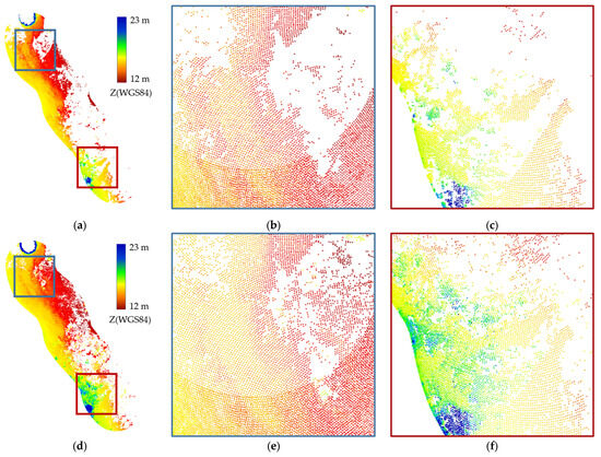
Figure 10.
Bottom point extraction results at test site 1: (a) overview of LBASSD result; (b,c): close-up views of boxes in (a); (d) overview of PGD result; (e,f): close-up views of boxes in (d).
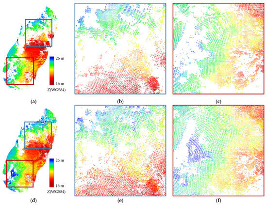
Figure 11.
Bottom point extraction results at test site 2: (a) overview of LBASSD result; (b,c): close-up views of boxes in (a); (d) overview of PGD result; (e,f): close-up views of boxes in (d).
4.3. Geolocation Accuracy Assessment
To evaluate the robustness of the proposed approach, the geolocation accuracy of the extracted bottom point clouds by PGD was compared with that of LBASSD, using echo-sounding data as the ground truth. The vertical distances (∆Z) between the bottom points and those from the echo-sounding data were calculated. Table 5 describes the mean error and standard deviation at each test site. The mean error of the PGD results (−0.315 m) at test site 1 decreased by 0.369 m compared to that of the LBASSD results (−0.684 m). On the other hand, the mean PGD error (0.109 m) at test site 2 slightly increased compared to that of the LBASSD result (0.033 m). Although the mean error is advantageous to use as a reference for measuring accuracy, it may be associated with characteristics of the Seahawk sensor system and a temporal difference between the ABL and echo-sounding data. The time differences between the acquisition of Seahawk and echo-sounding range from 3 to 4 months, during which changes in seafloor topography may have occurred. In particular, the negative mean ∆Z value at site 1 may indicate that the seafloor height had risen between the time of the echo-sounding survey (November 2021) and the Seahawk survey (March 2022), due to the deposition of eroded soil from the coast into the near sea. The mean ∆Z at site 2 may also be due to seafloor changes during the time gap (approximately 3 months), but the amount is negligible. From the ∆Z results calculated for the two sites, the trend and amount of variation (standard deviation) may be more meaningful than the mean values. The standard deviation of ∆Z, which reflects the robustness of the algorithm, did not differ significantly between LBASSD and the proposed approach at both sites. The ∆Z standard deviation of the PGD results was slightly higher than that of LBASSD at both test sites. However, considering that the number of bottom points extracted using PGD at each site increased by 18% and 14%, respectively, compared with the LBASSD results, the standard deviations of ∆Z are essentially the same.
Table 5.
Comparison of geolocation accuracy of bottom point clouds based on echo-sounding data.
5. Discussion
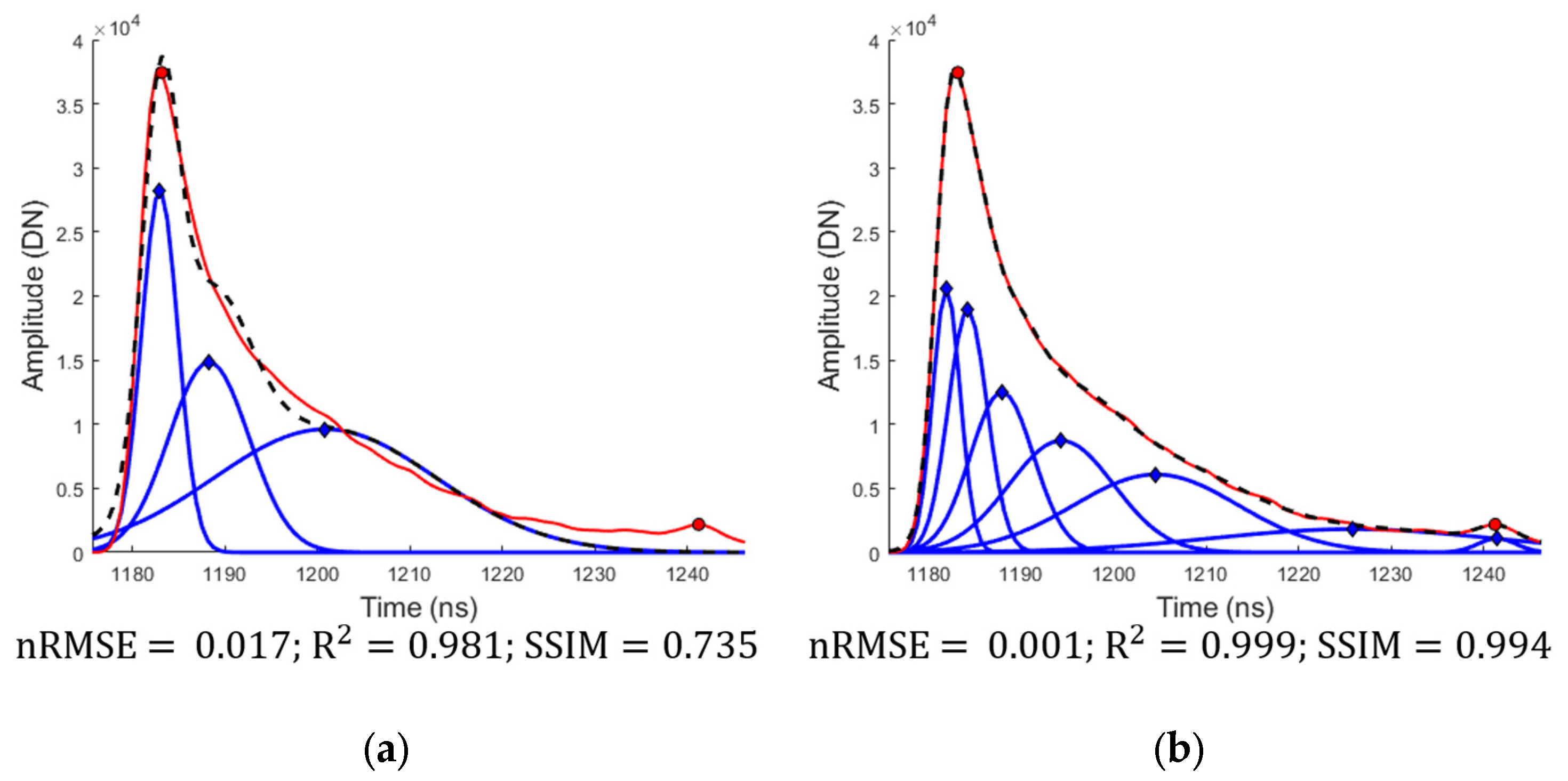
The proposed approach is designed to effectively approximate the original waveform with a Gaussian mixture model while ensuring that initially detected OPs are not missed and allowing for the estimation of potential returns that were not detected. The time difference between the OPs and EPs is utilized to determine whether the decomposed model sufficiently represents the original waveform. This criterion can prevent the neglect of low-intensity return components during Gaussian curve fitting. Figure 12a shows the decomposition results when only R2 > 0.95 was applied as the termination condition of iteration. The residual-based termination conditions inevitably include the possibility of missing weak returns. Figure 12b shows the results when the time difference criterion from the OP is used in addition to the R2 criterion. The results indicate that even a weak bottom return can be decomposed into components. However, it may be vulnerable in distinguishing noise from weak returns. If noise is falsely detected as a peak or if a weak peak that should have been detected is missed, incorrect decomposition could result. The limitation is related to noise removal performance, which can be improved through component verification with neighboring waveforms. Hence, this warrants further investigation.

Figure 12.
Comparison of waveform decomposition results in terms of termination criterion of iteration: (a) R2; (b) R2 and time difference between OP and EP.
The proposed approach can effectively decompose irregular and various ABL waveform types without a data-specific adjustment process. Existing ABL waveform decomposition techniques, which decompose the waveform into three fixed components (water surface, water column, and bottom), require separate classification and modeling for very shallow or deep water. However, PGD does not require such data-specific procedures or parameter adjustment according to the environment, thus simplifying and unifying the entire waveform processing. The approaches employing a fixed decomposition model can simultaneously label the water surface and bottom points during decomposition, but this is limited to typical ABL waveforms. Actual ABL data may include waveforms in which the bottom return is not received and noise may not be completely removed during waveform preprocessing. Consequently, whether the first component represents the water surface and the last one represents the bottom cannot be definitively determined. Therefore, we are investigating water labeling by utilizing various waveform features (e.g., amplitude, center, width, and return number) from the decomposed Gaussian components. The waveform features can also be used for classifying different underwater objects [18,44].
6. Conclusions
In this study, a new progressive waveform decomposition method based on the Gaussian mixture model is proposed to effectively decompose various ABL waveforms and improve the bathymetry performance. Experiments using the Seahawk waveform dataset acquired from different environments were conducted. The results confirmed that the proposed approach achieved superior performance in measuring bottom points compared with Seahawk’s data processing software by effectively detecting weak or shallow bottom returns. The proposed approach is universally applicable regardless of water depth, presence of unpredictable underwater objects, or irregular topography. In addition, it does not require a data-specific process according to the environment, thus simplifying the entire waveform processing. Furthermore, the proposed Gaussian decomposition technique can potentially be applied to various ABL bathymetry studies by enabling the extraction of diverse waveform features of the water surface, seafloor, and underwater points. Future works can include the investigation of the methods for overcoming noise misdetection and achieving the accurate automatic labeling of generated points.
Author Contributions
Conceptualization, H.K., M.J. and J.L.; methodology, H.K.; validation, H.K. and J.L.; formal analysis, H.K.; investigation, H.K. and M.J.; resources, G.W.; data curation, H.K. and G.W.; writing—original draft preparation, H.K. and M.J.; writing—review and editing, all authors; visualization, H.K.; supervision, J.L.; project administration, J.L.; funding acquisition, J.L. All authors have read and agreed to the published version of the manuscript.
Funding
This research was supported by Korea Institute of Marine Science & Technology (KIMST) funded by the Ministry of Oceans and Fisheries (RS-2023-00254717).
Institutional Review Board Statement
Not applicable.
Informed Consent Statement
Not applicable.
Data Availability Statement
The data presented in this study are available on request from the corresponding author.
Conflicts of Interest
The authors declare no conflict of interest.
References
- Klemas, V. Beach profiling and LIDAR bathymetry: An overview with case studies. J. Coast. Res. 2011, 27, 1019–1028. [Google Scholar] [CrossRef]
- Neal, J.; Hawker, L.; Savage, J.; Durand, M.; Bates, P.; Sampson, C. Estimating river channel bathymetry in large scale flood inundation models. Water Resour. Res. 2021, 57, e2020WR028301. [Google Scholar] [CrossRef]
- Wang, C.; Li, Q.; Liu, Y.; Wu, G.; Liu, P.; Ding, X. A comparison of waveform processing algorithms for single-wavelength LiDAR bathymetry. ISPRS J. Photogramm. Remote Sens. 2015, 101, 22–35. [Google Scholar] [CrossRef]
- Guenther, G.C. Airborne lidar bathymetry. In Digital Elevation Model Technologies and Applications: The Dem Users Manual, 2nd ed.; Maune, D.F., Ed.; ASPRS Publications: Bethesda, MD, USA, 2007; pp. 253–320. [Google Scholar]
- Hilldale, R.C.; Raff, D. Assessing the ability of airborne LiDAR to map river bathymetry. Earth Surf. Process. Landf. 2008, 33, 773–783. [Google Scholar] [CrossRef]
- Ducic, V.; Hollaus, M.; Ullrich, A.; Wagner, W.; Melzer, T. 3D vegetation mapping and classification using full-waveform laser scanning. In Proceedings of the Workshop on 3D Remote Sensing in Forestry, Vienna, Austria, 14–15 February 2006. [Google Scholar]
- Reitberger, J.; Schnörr, C.; Heurich, M.; Krzystek, P.; Stilla, U. Towards 3D mapping of forests: A comparative study with first/last pulse and full waveform LIDAR data. In Proceedings of the International Archives of Photogrammetry, Remote Sensing and Spatial Information Sciences, Beijing, China, 3–11 July 2008. [Google Scholar]
- Letard, M.; Collin, A.; Lague, D.; Corpetti, T.; Pastol, Y.; Ekelund, A.; Pergent, G.; Costa, S. Towards 3D mapping of seagrass meadows with topo-bathymetric lidar full waveform processing. In Proceedings of the 2021 IEEE International Geoscience and Remote Sensing Symposium IGARSS, Brussels, Belgium, 11–16 July 2021. [Google Scholar]
- Long, B.; Cottin, A.; Collin, A. What Optech’s bathymetric LiDAR sees underwater. In Proceedings of the 2007 IEEE International Geoscience and Remote Sensing Symposium IGARSS, Barcelona, Spain, 23–28 July 2007. [Google Scholar]
- Zhao, X.; Zhao, J.; Zhang, H.; Zhou, F. Remote sensing of suspended sediment concentrations based on the waveform decomposition of airborne LiDAR bathymetry. Remote Sens. 2018, 10, 247. [Google Scholar] [CrossRef]
- Richter, K.; Maas, H.G.; Westfeld, P.; Weiß, R. An approach to determining turbidity and correcting for signal attenuation in airborne lidar bathymetry. PFG—J. Photogramm. Remote Sens. Geoinf. Sci. 2017, 85, 31–40. [Google Scholar] [CrossRef]
- Wagner, W.; Ullrich, A.; Melzer, T.; Briese, C.; Kraus, K. From single-pulse to full-waveform airborne laser scanners: Potential and practical challenges. In Proceedings of the International Archives of Photogrammetry, Remote Sensing and Spatial Information Sciences, Istanbul, Turkey, 12–23 July 2004. [Google Scholar]
- Roncat, A.; Wagner, W.; Melzer, T.; Ullrich, A. Echo detection and localization in full-waveform airborne laser scanner data using the averaged square difference function estimator. Photogramm. J. Finl. 2008, 21, 62–75. [Google Scholar]
- Abdallah, H.; Bailly, J.S.; Baghdadi, N.N.; Saint-Geours, N.; Fabre, F. Potential of space-borne LiDAR sensors for global bathymetry in coastal and inland waters. IEEE J. Sel. Top. Appl. Earth Obs. Remote Sens. 2012, 6, 202–216. [Google Scholar] [CrossRef]
- Abady, L.; Bailly, J.S.; Baghdadi, N.; Pastol, Y.; Abdallah, H. Assessment of quadrilateral fitting of the water column contribution in lidar waveforms on bathymetry estimates. IEEE Trans. Geosci. Remote Sens. 2013, 11, 813–817. [Google Scholar] [CrossRef]
- Liu, G.; Ke, J. End-to-End Full-Waveform Echo Decomposition Based on Self-Attention Classification and U-Net Decomposition. IEEE J. Sel. Top. Appl. Earth Obs. Remote Sens. 2022, 15, 7978–7987. [Google Scholar] [CrossRef]
- Lai, X.; Yuan, Y.; Li, Y.; Wang, M. Full-waveform LiDAR point clouds classification based on wavelet support vector machine and ensemble learning. Sensors 2019, 19, 3191. [Google Scholar] [CrossRef] [PubMed]
- Kogut, T.; Slowik, A. Classification of airborne laser bathymetry data using artificial neural networks. IEEE J. Sel. Top. Appl. Earth Obs. Remote Sens. 2021, 14, 1959–1966. [Google Scholar] [CrossRef]
- Lowell, K.; Calder, B. Extracting shallow-water bathymetry from lidar point clouds using pulse attribute data: Merging density-based and machine learning approaches. Mar. Geod. 2021, 44, 259–286. [Google Scholar] [CrossRef]
- Shaker, A.; Yan, W.Y.; LaRocque, P.E. Automatic land-water classification using multispectral airborne LiDAR data for near-shore and river environments. ISPRS J. Photogramm. Remote Sens. 2019, 152, 94–108. [Google Scholar] [CrossRef]
- Liang, G.; Zhao, X.; Zhao, J.; Zhou, F. Feature selection and mislabeled waveform correction for water–land discrimination using airborne infrared laser. Remote Sens. 2021, 13, 3628. [Google Scholar] [CrossRef]
- Hofton, M.A.; Minster, J.B.; Blair, J.B. Decomposition of laser altimeter waveforms. IEEE Trans. Geosci. Remote Sens. 2000, 38, 1989–1996. [Google Scholar] [CrossRef]
- Chauve, A.; Mallet, C.; Bretar, F.; Durrieu, S.; Pierrot-Deseilligny, M.; Puech, W. Processing full-waveform lidar data: Modelling raw signals. In Proceedings of the ISPRS Workshop Laser Scanning and SilviLaser (LS SL), Espoo, Finland, 12–14 September 2007. [Google Scholar]
- Mallet, C.; Bretar, F. Full-waveform topographic lidar: State-of-the-art. ISPRS J. Photogramm. Remote Sens. 2009, 64, 1–16. [Google Scholar] [CrossRef]
- Guo, K.; Xu, W.; Liu, Y.; He, X.; Tian, Z. Gaussian half-wavelength progressive decomposition method for waveform processing of airborne laser bathymetry. Remote Sens. 2017, 10, 35. [Google Scholar] [CrossRef]
- Ding, K.; Li, Q.; Zhu, J.; Wang, C.; Guan, M.; Chen, Z.; Yang, C.; Liao, J. An improved quadrilateral fitting algorithm for the water column contribution in airborne bathymetric lidar waveforms. Sensors 2018, 18, 552. [Google Scholar] [CrossRef]
- Xing, S.; Wang, D.; Xu, Q.; Lin, Y.; Li, P.; Jiao, L.; Zhang, X.; Liu, C. A depth-adaptive waveform decomposition method for airborne LiDAR bathymetry. Sensors 2019, 19, 5065. [Google Scholar] [CrossRef]
- Schwarz, R.; Mandlburger, G.; Pfennigbauer, M.; Pfeifer, N. Design and evaluation of a full-wave surface and bottom-detection algorithm for LiDAR bathymetry of very shallow waters. ISPRS J. Photogramm. Remote Sens. 2019, 150, 1–10. [Google Scholar] [CrossRef]
- Zhu, J.; Zhang, Z.; Hu, X.; Li, Z. Analysis and application of LiDAR waveform data using a progressive waveform decomposition method. In Proceedings of the International Archives of the Photogrammetry, Remote Sensing and Spatial Information Sciences, Calgary, AB, Canada, 29–31 August 2011. [Google Scholar]
- Mountrakis, G.; Li, Y. A linearly approximated iterative Gaussian decomposition method for waveform LiDAR processing. ISPRS J. Photogramm. Remote Sens. 2017, 129, 200–211. [Google Scholar] [CrossRef]
- Oliveira, A.A.A.D.; Centeno, J.A.S.; Hainosz, F.S. Point cloud generation from Gaussian decomposition of the waveform laser signal with genetic algorithms. Bol. Ciên. Geod. 2018, 24, 270–287. [Google Scholar] [CrossRef]
- Kim, H.; Tuell, G.H.; Park, J.Y.; Brown, E.; We, G. Overview of SEAHAWK: A bathymetric LiDAR airborne mapping system for localization in Korea. J. Coast. Res. 2019, 91, 376–380. [Google Scholar] [CrossRef]
- Korea Marine Environment Management Corporation. Annual Report of the National Oceanographic Ecosystem; Ministry of Maritime Affairs and Fisheries: Sejong, Republic of Korea, 2020.
- Woo, K.S.; Sohn, Y.K.; Yoon, S.H.; Ahn, U.S.; Yoon, S.H.; Spate, A. Geology of Jeju Island. In Jeju Island Geopark—A Volcanic Wonder of Korea; Springer Science & Business Media: Berlin, Germany, 2013; pp. 13–14. [Google Scholar]
- Saylam, K.; Hupp, J.R.; Averett, A.R.; Gutelius, W.F.; Gelhar, B.W. Airborne lidar bathymetry: Assessing quality assurance and quality control methods with Leica Chiroptera examples. Int. J. Remote Sens. 2018, 39, 2518–2542. [Google Scholar] [CrossRef]
- Zhao, X.; Liang, G.; Liang, Y.; Zhao, J.; Zhou, F. Background noise reduction for airborne bathymetric full waveforms by creating trend models using Optech CZMIL in the Yellow Sea of China. Appl. Opt. 2020, 59, 11019–11026. [Google Scholar] [CrossRef]
- Yang, F.; Qi, C.; Su, D.; Ding, S.; He, Y.; Ma, Y. An airborne LiDAR bathymetric waveform decomposition method in very shallow water: A case study around Yuanzhi Island in the South China Sea. Int. J. Appl. Earth Obs. Geoinf. 2022, 109, 102788. [Google Scholar] [CrossRef]
- El-Sheimy, N.; Nassar, S.; Noureldin, A. Wavelet de-noising for IMU alignment. IEEE Aerosp. Electron. Syst. Mag. 2004, 19, 32–39. [Google Scholar] [CrossRef]
- Huang, L.; Kemao, Q.; Pan, B.; Asundi, A.K. Comparison of Fourier transform, windowed Fourier transform, and wavelet transform methods for phase extraction from a single fringe pattern in fringe projection profilometry. Opt. Laser Eng. 2010, 48, 141–148. [Google Scholar] [CrossRef]
- Jutzi, B.; Stilla, U. Range determination with waveform recording laser systems using a Wiener Filter. ISPRS J. Photogramm. Remote Sens. 2006, 61, 95–107. [Google Scholar] [CrossRef]
- MATLAB Documentation: Findpeaks. Available online: https://mathworks.com/help/signal/ref/findpeaks.html (accessed on 1 March 2023).
- MATLAB Documentation: Fit. Available online: https://mathworks.com/help/curvefit/fit.html?s_tid=srchtitle_fit_1 (accessed on 1 March 2023).
- Wang, Z.; Bovik, A.C.; Sheikh, H.R.; Simoncelli, E.P. Image quality assessment: From error visibility to structural similarity. IEEE Trans. Image Process. 2004, 13, 600–612. [Google Scholar] [CrossRef] [PubMed]
- Wang, M.; Wu, Z.; Yang, F.; Ma, Y.; Wang, X.H.; Zhao, D. Multifeature extraction and seafloor classification combining LiDAR and MBES data around Yuanzhi Island in the South China Sea. Sensors 2018, 18, 3828. [Google Scholar] [CrossRef] [PubMed]

Disclaimer/Publisher’s Note: The statements, opinions and data contained in all publications are solely those of the individual author(s) and contributor(s) and not of MDPI and/or the editor(s). MDPI and/or the editor(s) disclaim responsibility for any injury to people or property resulting from any ideas, methods, instructions or products referred to in the content. |
© 2023 by the authors. Licensee MDPI, Basel, Switzerland. This article is an open access article distributed under the terms and conditions of the Creative Commons Attribution (CC BY) license (https://creativecommons.org/licenses/by/4.0/).