On the Arrays Distribution, Scan Sequence and Apodization in Coherent Dual-Array Ultrasound Imaging Systems

Abstract

Coherent multi-transducer ultrasound (CoMTUS) imaging creates an extended effective aperture through the coherent combination of multiple arrays, which results in images with enhanced resolution, extended field-of-view, and higher sensitivity. However, this also creates a large discontinuous effective aperture that presents additional challenges for current beamforming methods. The discontinuities may increase the level of grating and side lobes and degrade contrast. Also, direct transmissions between multiple arrays, happening at certain transducer relative positions, produce undesirable cross-talk artifacts. Hence, the position of the transducers and the scan sequence play key roles in the beamforming algorithm and imaging performance of CoMTUS. This work investigates the role of the distribution of the individual arrays and the scan sequence in the imaging performance of a coherent dual-array system. First, the imaging performance for different configurations was assessed numerically using the point-spread-function, and then optimized settings were tested on a tissue mimicking phantom. Finally, a subset of the proposed optimum imaging schemes was experimentally validated on two synchronized ULA OP-256 systems equipped with identical linear arrays. Results show that CoMTUS imaging performance can be enhanced by optimizing the relative position of the arrays and the scan sequence together, and that the use of apodization can reduce cross-talk artifacts without degrading spatial resolution. Adding weighted compounding further decreases artifacts and helps to compensate for the differences in the brightness across the image. Setting the maximum steering angle according to the spatial configuration of the arrays reduces the sidelobe energy up to 10 dB plus an extra 4 dB reduction is possible when increasing the number of PWs compounded.

1. Introduction

Ultrasound (US) imaging is a valuable medical diagnostic tool because of its safety, low cost and real-time imaging capability [1]. However, conventional US images are hampered by a restricted field of view (FOV), limited and anisotropic resolution, relatively low contrast, and limited depth penetration, becoming ever more critical as population rates of obesity rise [2]. All these limitations stem in one way or another from the reliance on handheld probes, specifically due to the limited spatial extent of their transmitting and receiving apertures [3,4]. In practice, the size of such handheld probes is limited by the need to operate with highly variable body shapes and, for some applications, limited or discontinuous acoustic windows. Nevertheless, larger apertures are desired to improve resolution, penetration, and FOV [3,5,6].

An ideal imaging system with a large and flexible aperture would have the potential to overcome the fundamental US limitations and lead to significant imaging improvements. However, fabrication of flexible probes that can conform to the body has not been successfully implemented because coherent image formation would require continuous estimation of the transducer shape. Previous attempts at flexible arrays are mostly restricted to nondestructive testing and evaluation of specimens that are still and with simple geometries [7], and the transducer shape calibration relies on external positional sensors [8]. Alternative methods based on image contrast or entropy optimization have also been investigated in medical US but they have been only tested for small linear arrays and homogeneous media [9,10]. One way to extend the aperture of the imaging system while keeping some geometrical flexibility is coherent multi-transducer ultrasound (CoMTUS) imaging [11]. CoMTUS enables the use of multiple synchronized arrays, which take turns to transmit plane waves (PWs) into a common FOV, and together acting as one large effective aperture. Coherent combination of all signals received by the extended aperture improves resolution and sensitivity, and extends the FOV, while flexible placement of individual arrays preserves compatibility with different body shapes and parallel operation can preserve time resolution. In contrast to previous works on multiple probes that rely on a fixed geometry [12,13,14,15], CoMTUS utilizes multiple standard US arrays that can be positioned flexibly and combined into an extended dynamically self-calibrating large aperture. This calibration is done by optimizing the beamforming parameters: the average sound speed in the medium, and the location of the transducers [11]. This also provides improved tolerance for imaging acoustically heterogeneous tissue with a large aperture [16]. The method has been experimentally demonstrated using two probes; initially with 1D (linear) arrays that were constrained to lie in a common plane [11,16], and more recently 2D sparse arrays were used to demonstrate the feasibility of 3D CoMTUS imaging [17].

Nevertheless, the large discontinuous aperture created by CoMTUS presents challenges for existing beamforming algorithms, developed for small and continuous apertures [18,19]. Indeed, preliminary findings have shown that CoMTUS imaging performance is affected by the discontinuous effective aperture distribution and the scan sequence [16]. For example, increased separation between the transducers can extend the aperture and improve resolution, however, these discontinuities can reduce contrast due to grating and side lobes. Furthermore, the use of multiple synchronized arrays can result in interactions among the beams and possible direct transmissions between the individual arrays that generate undesirable cross-talk artifacts. Like in coherent PW imaging [20], in CoMTUS it is expected that coherently compounding the images obtained from the transmission of multiple steered PWs may reduce the amplitude of side lobes and thus, improve contrast. However, it is unclear how much the interplay between the discontinuities and the scan sequence affect the global performance of the method. If the scan sequence is not properly preset according to the spatial configuration of the arrays, these factors might have a negative impact on CoMTUS performance. Likewise, the apodization laws also play an important role in imaging quality [21]. For example, in multi-line transmit beamforming, where the images suffer from inter-beam cross-talk artifacts, the use of a Tukey apodization window in both transmission and receive lowers the cross-talk artifacts, however, at the expense of lateral resolution [22,23]. It is yet unclear what the corresponding trade-offs are for CoMTUS.

The aim of this work is to investigate, both in simulation and experimentally, the role of the distribution of the individual arrays, scan sequence, and apodization on CoMTUS image quality, and specifically to explore how to attain the best point spread function (PSF) images with either minimum-side lobe energy (an indicator of contrast) or minimum main lobe width (an indicator of resolution) and the highest frame rate possible. For the first time, this study explores the imaging performance of coherent dual-array systems, taking into account the relative position between arrays, the scan sequence, and the apodization. The cross-talk artifacts are also investigated for the first time in this context. This work can, thus, provide a guideline to determine imaging performance trade-offs in different applications and to guide further studies on multi-transducer beamforming.

2. Materials and Methods

2.1. Coherent Dual-Array Imaging

A CoMTUS imaging system, created using two identical linear arrays (LA332, Esaote, Firenze, Italy), was investigated using both simulations and experiments. Each array had 144 active elements, a pitch of 245 μm, a central frequency of 3 MHz, and 80% bandwidth. The arrays were constrained to share an overlapping FOV in the same elevational plane. A transmission imaging sequence was implemented in which both arrays take turns to transmit a PW while simultaneously receiving the backscattered echoes. Note that, compared to a single probe system using the same imaging sequence, the frame rate would be halved. The notation $T_i{R}_j$ was used to denote radiofrequency (RF) data received by array j when array i transmits.

The beamforming process for this coherent dual-array system is described in detail in [11]. Briefly, delay and sum beamforming was applied to each received RF dataset in the same coordinate system [20]. Here, delays accounted for the complete pathway between the transmit array and the receive elements. Then, a CoMTUS image is generated by coherently summing all beamformed data for all transmissions and all receivers. Finally, the delayed and compounded signals are envelope detected and log-compressed.

As shown in Figure 1, the relative position of the two arrays was defined by the angle between the axes of the arrays, θ, and the gap between the arrays, which consequently define the imaging depth defined at the center of the common FOV of both arrays. The scan sequence was defined by the maximum steering angle, α_max, and the number of transmitted PWs. The specific steering angle of PWs was determined in linear steps between −α_max and α_max. The transducers were excited using a Gaussian-windowed 3-cycle sinusoidal burst at 3 MHz. CoMTUS images were beamformed in the coordinate system of the resulting effective aperture (Figure 1). This is the coordinate system defined at the center of the extended aperture created by the two arrays, where the best spatial resolution is aligned with the x-axis (3). To reduce artifacts, different apodizations were investigated on transmit: rectangular window (no apodization) and 50%-Tukey window. A rectangular window was used on receive. This specific window (Tukey) was chosen because it is flat for the majority of the window length, which allows the propagation of a plane wavefront for a long depth of field with very limited diffraction [24]. Moreover, Tukey apodization was previously shown effective to better reduce the cross-talk artifacts in multi-line transmit beamforming when compared to other window functions [22,23].

2.2. Simulations

Simulations were performed to study the effect of the spatial position of the two arrays and the scan sequence on the imaging performance of the system. The configurations were simulated in MATLAB (The MathWorks, Natick, MA, USA) by using Field II [25,26], setting a sampling frequency of 100 MHz.

Two different sets of simulations were performed. The first set consisted of an optimization sweep, in which the parameters were varied to evaluate the configuration where CoMTUS operates most effectively. A single point-scatterer was placed at the center of the common FOV of both arrays (see Figure 1) to simulate the system PSF for different spatial configurations, depths, and using different numbers of angled transmissions at varying angle ranges. Each parameter was allowed to vary as follows: the angle between the arrays, θ: 95° to 165°; the gap between the arrays: 0 mm to 35 mm; the maximum transmitted PW angle, α_max: 0° to 15°; the number of transmitted PWs per array: 1 to 11. The ranges of the parameters investigated were chosen to match feasible experimental configurations of the two arrays. In a first step, the optimum α_max was determined as a function of depth. Like in standard PW compounding with a single array, it is expected that α_max decreases with depth [20]. To optimize α_max, a simulation was performed varying α_max from 0° to 15° while keeping the number of transmissions per array equal to 3, (−α_max, 0°, α_max), and the gap between the arrays zero. This results in a total of six PWs to be compounded in CoMTUS images. The angle between the arrays was varied according to the desired depth. In a second step, a simulation was performed varying the number of PWs for the different probe positions (changing angle and gap) while α_max was set according to the imaging depth (resulting from the previous step).

PSFs were used to determine two optimal configurations at 70 mm depth: a first configuration with minimum-side lobe energy, and a second configuration with a minimum main lobe width. The latter configurations were used for a second set of simulations investigating a tissue-mimicking phantom. The phantom consisted of randomly generated point scatterers (234 scatterers/mm³) with a Gaussian amplitude distribution, along with a 10-mm diameter circular empty region simulating an anechoic cyst. The tissue phantom size was 50 mm (width) × 1 mm (depth) × 30 mm (height) and was centered at a depth of 70 mm from the center of both arrays. This phantom was used to demonstrate the effectiveness of the imaging configuration in determining edges of regions and the impact of grating and side lobe on the final image quality. Simulations were performed using 7 transmission angles per array with a maximum steering angle of 13°. These choices are based on the previous optimization and will be explained further in Section 3.

2.3. Experiments

To experimentally validate the schemes proposed by the simulation study, a subset of the imaging schemes outlined in Section 2.1 were implemented on two 256-channel Ultrasound Advanced Open Platform (ULAOP 256) systems (MSD Lab, University of Florence, Florence, Italy) [27] equipped with a pair of the above-mentioned linear array probes (Esaote LA332). The systems were synchronized in both transmit and receive by sharing the same trigger and sampling times and were used to operate each individual probe [28]. Both probes were mounted on xyz translation and rotation stages (Thorlabs, Newton, NJ, USA) to allow for careful alignment in the elevational plane to enable imaging of a common region of interest. For each probe, in an alternating sequence, a total of 7 PWs with a maximum steering angle (α_max) of 13° were transmitted at 3 MHz with pulse repetition frequency (PRF) of 1 kHz. Two apodization windows, rectangular and a 50%-Tukey, were tested in transmit. Raw data were acquired simultaneously by both arrays at a sampling frequency of 19.5 MHz and then post-processed in MATLAB to perform the coherent image reconstruction. To further reduce experimental artifacts, two weighted compounding schemes were implemented: a rectangular window, in which all RF datasets acquired are weighted the same ($\frac{1}{4}\left[T_1{R}_1+T_1{R}_2+T_2{R}_1+T_2{R}_2\right])$, and a second case when the trans-received data (data obtained when the transmit and receive arrays are different) is weighted half the weighting applied to the data where the trans-receive array is the same $\left(\frac{1}{6}\left[2\times T_1{R}_1+T_1{R}_2+T_2{R}_1+2\times T_2{R}_2\right]\right)$. The latter weighted compounding was used to keep the brightness of the reflections in the common FOV approximately constant, since the backscattered echoes of the trans-received data appear at approximately the same location resulting in a final CoMTUS image with greater brightness in the common FOV.

In a first experiment, the probes were immersed in water and the resulting direct transmissions were acquired at two different spatial configurations: defined at 40 mm imaging depth with θ = 120° and gap = 9.6 mm, and at 90 mm imaging depth with θ = 150° and gap = 23.7 mm.

In a second experiment, a calibrated commercial phantom (CIRS Multi-Purpose, Multi-Tissue Ultrasound Phantom model 040GSE with speed of sound 1540 m/s and attenuation 0.7 dB/cm/MHz) was used to experimentally validate the method by assessing the image metrics (see Section 2.4). Water was inserted between the arrays and the flat surface of the commercial phantom to ensure acoustic coupling. Note that the coupling water had a different speed of sound than the phantom, which may introduce aberrating effects. The two probes were positioned to image a common region of interest located at 70 mm depth and following approximately the two spatial configurations investigated in the tissue-mimicking phantom simulations, i.e., a configuration with minimum-side lobe energy and a configuration with minimum main lobe width.

2.4. Image Quality Metrics

PSF images were used to calculate the lateral full-width at half-maximum (FWHM) to give an indication of the resolution, and the peak side-to-main lobe ratio (PSMR) and side-to-main lobe energy ratio (SMER) to assess the artifacts [29]. The PSMR was determined by the ratio between the amplitude of the maximum side peak to the amplitude of the main lobe. The SMER was defined as the sum of the intensity of the sidelobes, divided by the sum of the intensity of the main lobe, where the cutoff points for the main lobes and side lobes were −6 dB, and between −40 and −6 dB respectively. Thus, the SMER is given by,

$$\mathrm{S}\mathrm{M}\mathrm{E}\mathrm{R}=20{\log }_{10}\left(\frac{{\int }_{-40\mathrm{d}\mathrm{B}}^{-6\mathrm{d}\mathrm{B}}\mathrm{I}\left(\overrightarrow{\mathrm{r}}\right)\mathrm{d}\overrightarrow{\mathrm{r}}}{{\int }_{-6\mathrm{d}\mathrm{B}}^{0\mathrm{d}\mathrm{B}}\mathrm{I}\left(\overrightarrow{\mathrm{r}}\right)\mathrm{d}\overrightarrow{\mathrm{r}}}\right)$$

(1)

where $\mathrm{I}\left(\overrightarrow{\mathrm{r}}\right)$ is the intensity of a pixel located at position $\overrightarrow{\mathrm{r}}$.

The maximum imaging depth affected by the cross-talk artifacts generated by direct transmissions was estimated as half of the distance between the extreme elements of both arrays (first element for probe 1 and last element for probe 2 (gray horizontal line in Figure 1)). The energy of the direct transmissions was quantified by summing the squared amplitudes of the trans-receive RF data acquired in the water tank and converting to decibel units.

To evaluate the image quality of the tissue-mimicking phantom, four further imaging metrics were used: the speckle resolution, calculated from the autocorrelation function of a speckle region as the FWHM of the Gaussian-fitted curve; the contrast ratio (CR); contrast-to-noise ratio (CNR); and the generalized contrast-to-noise ratio (gCNR) [30],

$$CR=20{\log }_{10}\left(\frac{{\mu }_i}{{\mu }_o}\right)$$

(2)

$$CNR=\frac{\left|{\mu }_i-{\mu }_o\right|}{\sqrt{{\sigma }_i^2+{\sigma }_o^2}}$$

(3)

$$gCNR=1-OVL$$

(4)

where ${\mu }_i$ and ${\mu }_o$ are the means of the signal in a region of interest (ROI) inside and outside of the anechoic cyst, respectively, ${\sigma }_i$ and ${\sigma }_o$ are the corresponding standard deviations of the signals in the ROIs, and OVL is the overlap area between the probability density functions of both ROI signals [30].

3. Results

3.1. Simulation Results

The imaging depth, common FOV area, and the theoretical maximum depth affected by the cross-talk artifacts generated by the direct transmissions were calculated for the different configurations defined in Section 2.2. Figure 2 shows the relationships between the investigated parameters. The targeted imaging depth increases at larger angles and separation between the arrays; the area of the common FOV does not depend on the gap between the arrays and increases with the angle between them, while the maximum depth affected by cross-talks is mostly dictated by the gap between the arrays. For the considered ranges of parameters, the imaging depth ranges from 19 mm to 267 mm, the area of the common FOV from 1232 mm² to 4742 mm², and the theoretical depth affected by the cross-talk artifacts ranges from 26 mm to 52 mm.

The effects of α_max on the PSF are shown in Figure 3, where the lateral FWHM, PSMR and SMER are displayed as a function of the imaging depth, angle between arrays, and α_max, keeping the number of transmissions per array equal to 3, (−α_max, 0°, α_max), and the gap between the arrays equal to zero. These results show that, for a continuous aperture (gap = 0), PSMR and SMER decrease at larger steering angles, while the FWHM does not depend strongly on α_max and, as expected, deteriorates with increasing imaging depth. While for each imaging depth PSMR and SMER have a clear minimum (<−25 dB and <2 dB, respectively, dark blue regions in Figure 3b,c) that corresponds to a certain α_max, steering the transmitted PW does not produce any significant effect on the main lobe width (Figure 3). These results suggest that for the best trade-off, α_max can be determined by minimizing both PSMR and SMER at the desired imaging depth. The locus of these values is indicated by the white line in Figure 3.

The effect of the number of transmitted PWs on the image metrics is depicted in Figure 4, where α_max was set according to the imaging depth (white line in Figure 3). The extreme simulated cases with the minimum (3 PWs) and maximum (11 PWs) number of transmitted PWs per array are shown. For the other cases with 5, 6, 7 and 9 PWs the metrics follow the same trends with values in between. Since θ and thus depth is the main determinant of FWHM and the gap between the arrays plays the main role for PSMR and SMER, averaged results over the gap and over the angle between transducers are shown for FWHM, and PSMR and SMER, respectively (Figure 4 bottom row). FWHM and PSMR do not depend on the number of transmitted PWs, and SMER improves (lower values) with increasing transmissions, reaching a plateau after about 5 PWs.

Figure 5 shows the different metrics as a function of the angle and the separation between the arrays, where α_max was set according to the imaging depth (chosen using Figure 3) and the number of transmitted PWs per array to 7 (chosen to ensure stable (plateau) performance using Figure 4). Note that 7 PWs is the next number of transmissions investigated after the minimum one obtained from Figure 4 and was chosen as a conservative solution. In agreement with previous results, PSMR and SMER mainly depend on the gap between the arrays, worsening at larger gaps, while FWHM depends on the angle between the transducers, which mainly dictates the imaging depth together, to a minor extent, with the gap (Figure 1). At large θ, PSMR and SMER are more sensitive to changes in the gap between the arrays. Note that, as indicated in the figure captions, Figure 3, Figure 4 and Figure 5 display results obtained with Tukey apodization on transmit. Similar trends were observed for the case of no apodization (rectangular window), so are not shown here. Thus, the selected configurations do not change with the transmit apodization.

From these results and at certain imaging depth, it is possible to identify two extreme configurations, i.e., a first configuration with minimum-side lobe energy, and a second configuration with a minimum main lobe width. These two configurations and their corresponding metrics at 70 mm depth are indicated with a white dot and a white star, respectively, in Figure 5.

Figure 6 shows an example of the PSF and its lateral cross-section for a numerical point scatterer at 70 mm depth using the two extreme geometries (minimum-side lobe energy (Figure 6a,b) and minimum main lobe width (Figure 6c,d)) and with the different apodization laws used on transmit (rectangular (Figure 6a,c) and Tukey (Figure 6b,d) windows). The corresponding imaging metrics are summarized in

Table 1. Imaging metrics at 70 mm depth for parameters chosen to obtain images with minimum-side lobe energy (array configuration: θ = 149°, gap = 3 mm) and with minimum main lobe width (array configuration θ = 124°, gap = 35 mm) and using rectangular or Tukey apodization on transmit (Tx). FWHM, PSMR and SMER are calculated from the PSFs in Figure 6. CR, CNR, gCNR and speckle size are calculated from the numerical B-mode images in Figure 7.

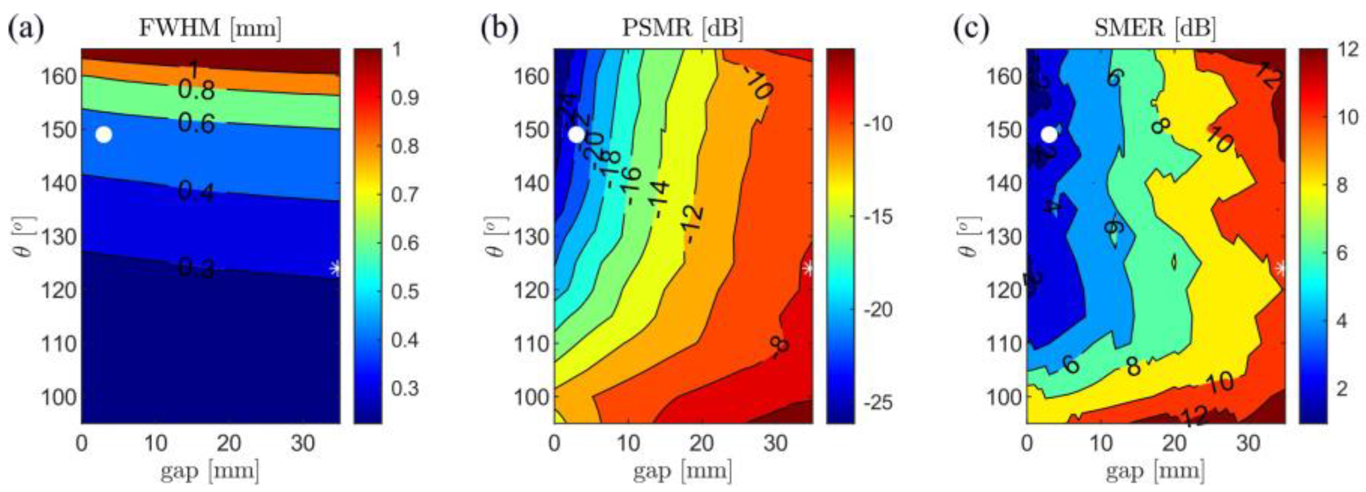
Configuration	θ = 149°, gap = 3 mm (Minimum-Side Lobe Energy)		θ = 124°, gap = 35 mm (Minimum Main Lobe Width)
Tx. Apodization	Rectangular	Tukey	Rectangular	Tukey
FWHM [mm]	0.49	0.49	0.29	0.29
PSMR [dB]	−23.7	−20.7	−8.3	−7.2
SMER [dB]	0.0	0.9	9.4	10.3
CR [dB]	−22.7	−22.6	−23.4	−23.6
CNR [-]	1.65	1.64	1.72	1.72
gCNR [-]	0.97	0.97	0.97	0.97
Speckle resolution [mm]	0.53	0.54	0.38	0.38

. Minimum-side lobe amplitude results in PSMR up to 16.5 dB lower than minimum main lobe width, but worse resolution (0.49 mm vs. 0.29 mm). The use of apodization on transmit only affects the metrics PSMR and SMER, and no others. Compared to a transmit rectangular apodization, when a Tukey law is used on transmit, the PSMR increases by 3 dB and 1.1 dB in the minimum-side lobe energy and minimum main lobe width configuration, respectively, while SMER increases by 0.9 dB in both configurations. Although the amplitude of the first side lobe is higher on Tukey apodization, the images of the point scatterer look more refined because the second side lobe amplitudes are much smaller (Figure 6e).

The B-mode images of the tissue-mimicking phantom using the proposed configurations at 70 mm depth and with Tukey apodization on transmit are shown in Figure 7. The lateral section of the anechoic region (Figure 7c) shows that the mean gray level inside is similar in both cases. Using these configurations, the inclusion is visible with a CR of −22.7 dB, CNR of 1.65, and gCNR of 0.97 in the minimum-side lobe energy case vs. −23.4dB, 1.72 CNR, and 0.97 gCNR in the minimum main lobe width case. Significant differences in the speckle texture can be appreciated between Figure 7a,b, relating to minimum-side lobe energy and minimum main lobe width configurations, respectively. The latter, in agreement with the resolution measured from the PSF, produces a thinner speckle size and better-defined edges, making Figure 7b more resolute than Figure 7a. Table 1 shows the imaging metrics for both configurations and transmit apodization laws. Based on calculations in Table 1, the use of apodization on transmit does not affect any of the contrast metrics.

3.2. Experimental Results

Examples of the resulting direct transmissions between arrays experimentally measured at 40 mm depth (θ = 120° and gap = 9.6 mm) in a water tank are shown in Figure 8, where the rectangular and Tukey apodization laws in transmit are compared. The use of a Tukey window on transmit reduced the length of the direct transmissions between arrays, from approximately 50 µs (38.5 mm depth) to 43.5 µs (33.5 mm depth), which approximately matches the value predicted by the simulation (Figure 2c). The energy of the direct transmissions was also reduced by the Tukey window by 6.7 dB (146.5 dB vs. 139.8 dB). Similar results were observed for different probe configurations and imaging depths.

B-mode images of the calibrated commercial phantom (CIRS 040GSE) above the hypoechoic cysts and above the wire targets are shown in Figure 9 for the configurations of minimum-side lobe energy (θ = 147.57° and gap = 7.3 mm) and in Figure 10 for the minimum main lobe width (θ = 127.79° and gap = 32.6 mm). The images were obtained after the optimization of the beamforming parameters as described in [11], and using the point-targets of the shared FOV. The targets used for optimization are marked in Figure 9 and Figure 10 with dashed lines. Note that, due to finite tolerances of the experimental setup, the spatial configurations slightly differ from the theoretical ones used in the simulations. In agreement with the simulations (Figure 2b) and due to a larger angle between transducers, the configuration of minimum-side lobe energy (Figure 9) produces images with a greater common FOV than the configuration of minimum main lobe width (Figure 10). Some of the artifacts resulting from direct transmissions between the arrays are indicated with red arrows in the first column (rectangular window). With a smaller gap between arrays (Figure 9), there are also less cross-talk artifacts as predicted in Figure 2c, and the hypoechoic cysts are easier to identify. For both configurations the wire targets within the common FOV of both arrays appear to have narrower main lobe width.

Different apodization laws are compared in Figure 9 and Figure 10, i.e., (Figure 9 and Figure 10a,d) rectangular apodization on transmit, (Figure 9 and Figure 10b,e) Tukey apodization on transmit, and (Figure 9 and Figure 10c,f) Tukey apodization on transmit plus weighting halved for the trans-received data for weighted compounding. Comparing the different apodization laws on transmit, overall, the Tukey law reduces cross-talk artifacts in both configurations, which are more significant and affect more depth (37.5 mm vs. 49 mm) in the minimum main lobe width configuration (Figure 10). Adding weighted compounding further decreases the observed artifacts and helps to compensate for the differences in the brightness across the image.

The speckle size was assessed from a rectangular region of 10 × 10 mm² centered at 73 mm depth from the images above the hypoechoic cysts. The corresponding results are shown in

Table 2. Imaging metrics from Figure 9 (minimum-side lobe energy, θ = 147.57° and gap = 7.3 mm) and Figure 10 (minimum main lobe width, θ = 127.79° and gap = 32.6 mm). Different apodization laws are compared: no apodization either on transmit or receipt (None), Tukey apodization on transmit (Tx), and Tukey apodization on transmit plus weighted compounding (Tx&Rx).

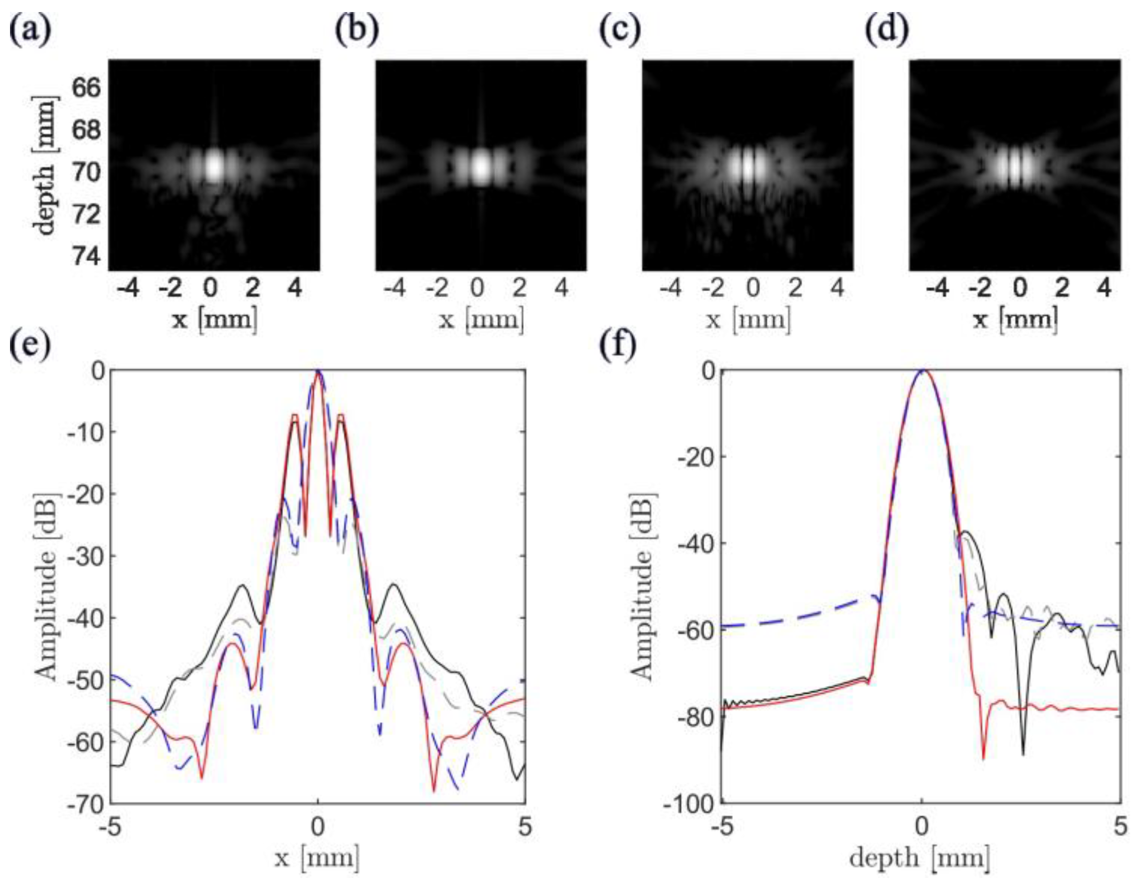
Configuration	θ = 149°, gap = 3 mm (Minimum-Side Lobe Energy)			θ = 124°, gap = 35 mm (Minimum Main Lobe Width)
Tx. Apodization	None	Tukey	Tukey	None	Tukey	Tukey
Weighted compounding	No	No	Yes	No	No	Yes
Speckle size [mm]	0.40	0.40	0.37	0.28	0.30	0.26

. As expected, the minimum main lobe width configuration presents a thinner speckle size than the minimum-side lobe energy configuration, being the case with apodization in transmit plus weighted compounding the one with the smallest speckle size in both configurations.

4. Discussion

This study investigates CoMTUS performance as the geometry of a coherent dual-array system, the scan sequence and the apodization laws applied in transmit. Both simulations and in vitro experiments are reported. From the PSF simulations, a general sense of the optimum scan sequence at each spatial configuration can be determined. Simulations showed that the spatial configuration of the different arrays determines the overall CoMTUS imaging performance, with different geometries favoring minimization of PSF main lobe width and side lobe energy (Figure 6). In general, resolution worsens with increasing angle between the arrays while the PSMR and SMER worsen because the amplitude of the side lobes rises at larger separations between the arrays (Figure 4 and Figure 5). The PSF results show that, unlike standard compounding PW imaging with a single probe where the steering angle determines the F-number and lateral resolution [20,31], CoMTUS resolution is imposed by the size of the large effective aperture created, rather than the largest PW angle transmitted (Figure 3). Compounding PWs at varying angles may aid in reducing the side lobe energy (Figure 4). This suggests that both the relative location of the individual probes and the PW transmission angles are directly related and either one or both can determine the achievable resolution and contrast in the final image. This presents the opportunity to adaptively change imaging performance by using the relative location of the arrays to select the range of PW angles to use. For most applications, imaging will be performed in the center of the optimization sweep. This region is useful as the imaging depth is already significant and image quality can be maintained. Nevertheless, in practice, the imaging metrics will be affected by a complex combination of probe positions, aperture size, transmit PW angle, apodization law, and imaging depth. The relative location of the multiple arrays represents the main source of possible measurement uncertainties. These can be minimized by verifying and ensuring a perfect alignment between the scan planes by a preliminary assessment of the transmitted acoustic fields. Furthermore, the relative position of the multiple arrays and the scan sequence should be adapted to the specific application.

In terms of resolution, the calculations in Table 1 indicate, as expected, that a better resolution is achieved with the minimum main lobe width configuration. However, the significantly thinner main lobe also affects the speckle texture and the final lesion detection in B-mode images (Figure 7), presenting this configuration also better contrast metrics despite the worse PSMR and SMER. Given that the lesion and target detectability is a function of both the contrast and resolution [32,33], overall, the extended aperture size improves lesion detectability, even when the side lobes are significant. Figure 7 shows that a cyst located at the common FOV is better visible in the configuration with higher resolution and worse PSMR and SMER. A narrow main lobe permits fine sampling of high-resolution objects, providing improved boundary detection for clinically relevant targets. Early studies [16] show that, with limited separation between transducers, the extended aperture created by CoMTUS provides benefits in both resolution and contrast that improve image quality, particularly at large imaging depths, compared with a conventional single transducer system. This was demonstrated even in the presence of acoustic clutter caused by tissue layers of varying speed of sound.

The use of transmit apodization on CoMTUS reduces cross-talk artifacts (Figure 9 and Figure 10) but, in contrast to previous studies based on single arrays [22,23], without affecting the spatial resolution and speckle size (Table 1 and Table 2). Experimental results show that, despite the predicted improvements in resolution and target detectability, there are practical limitations to the gains made with CoMTUS, and these mostly depend on the spatial configuration of the arrays. While benefits in the common FOV of the arrays are evident in the calibration phantom (Figure 9 and Figure 10), other parts of the images may be degraded by artifacts created by grating lobes and direct transmissions between arrays. These effects are clearly visible in the configuration of minimum main lobe width (Figure 10), which presents the largest gap between arrays (32.6 mm vs. 7.3 mm) and so larger expected grating lobes. Advanced beamforming methods [34,35,36] to reduce side lobes and grating lobes [13,37] will be explored in the future to further improve CoMTUS performance. There is a complex interplay between FOV and imaging performance as arrays are moved relative to one another. The final CoMTUS image will always achieve an extended FOV; however, the resolution is only able to improve in overlapping regions. This improvement will be greatest toward the center, where the overlap includes transmission and reception for both transducers. Thus, the benefits may be of various kinds in different locations. Those spatial configurations that will maximize the overlapping FOV will lead to more uniform images with enhanced performance. However, the different experimental conditions (different areas of the CIRS phantom were imaged) make it difficult to provide a straightforward comparison between the two different configurations. Indeed, the restricted acoustic window of the phantom limits the position of the arrays and the accessible areas of the phantom, making it infeasible to image precisely the same region with both configurations. Likewise, in the future, a direct comparison of the in vitro images with their simulated counterpart could be used to further support these findings.

The wavefront aberration caused by the different speed of sound between the water (used for coupling) and the CIRS phantom is evident also in images acquired by a single array (images not shown). In the presence of sound speed variation, the effect of aberration is less pronounced in the common FOV of both arrays and close to the points used for calibration. However, the errors in the applicability of the calculated positions of the arrays and local speed of sound are likely to increase in regions further from the targets. These effects are visible in the targets around 20 mm depth in Figure 9 and Figure 10. More accurate sound speed estimation would improve beamforming [38] and also enable higher order phase aberration correction in the areas away from the calibration targets. In addition, the use of several probes allows multiple interrogations from different angles that may add extra benefits [39]. Finally, if different transmitted beams are used, such as divergent waves [40], there will be additional factors that could affect CoMTUS performance and should be considered [41]. In future studies, the use of apodization on receive to further improve image performance, and TX/RX strategies capable of increasing the achievable frame rate should be investigated.

5. Conclusions

In this work, the effects that the array spatial distribution, transmit PW sequence, and apodization law have on CoMTUS imaging performance have been investigated using both simulations and experiments. The findings show that CoMTUS spatial resolution is mostly defined by the size of the effective aperture created rather than the maximum transmitted PW angle, and that compounding PWs at different angles may aid in reducing side lobe energy. In addition, the use of apodization on transmit reduces the cross-talk artifacts without degrading spatial resolution and adding weighted compounding further decreases artifacts and helps to compensate the differences in the brightness across the image. Thus, an optimum relative location and scan sequence of the arrays can produce images with improved resolution while maintaining high-frame rates. In practice, the relative spatial position of the multiple arrays and the scan sequence should be adapted for the application. This study could be considered as a user’s guideline to quickly determine the imaging performance trade-off and compare with the specific application requirements.

References

- Fraleigh, C.D.M.; Duff, E. Point-of-Care Ultrasound: An Emerging Clinical Tool to Enhance Physical Assessment. Nurse Pract. 2022, 47, 14–20. [Google Scholar] [CrossRef] [PubMed]
- Tsai, P.J.S.; Loichinger, M.; Zalud, I. Obesity and the Challenges of Ultrasound Fetal Abnormality Diagnosis. Best Pract. Res. Clin. Obs. Gynaecol. 2015, 29, 320–327. [Google Scholar] [CrossRef] [PubMed]
- Cobbold, R.S. Foundations of Biomedical Ultrasound; Oxford University Press: New York, NY, USA, 2006. [Google Scholar]
- Jensen, J.A. Medical Ultrasound Imaging. Prog. Biophys. Mol. Biol. 2007, 93, 153–165. [Google Scholar] [CrossRef] [PubMed]
- Bottenus, N.; Long, W.; Zhang, H.K.; Jakovljevic, M.; Bradway, D.P.; Boctor, E.M.; Trahey, G.E. Feasibility of Swept Synthetic Aperture Ultrasound Imaging. IEEE Trans. Med. Imaging 2016, 35, 1676–1685. [Google Scholar] [CrossRef] [PubMed]
- Bottenus, N. Implementation of Constrained Swept Synthetic Aperture Using a Mechanical Fixture. Appl. Sci. 2023, 13, 4797. [Google Scholar] [CrossRef]
- Hunter, A.J.; Drinkwater, B.W.; Wilcox, P.D. Autofocusing Ultrasonic Imagery for Non-Destructive Testing and Evaluation of Specimens with Complicated Geometries. NDT E Int. 2010, 43, 78–85. [Google Scholar] [CrossRef]
- Lane, C.J.L. The Inspection of Curved Components Using Flexible Ultrasonic Arrays and Shape Sensing Fibres. Case Stud. Nondestruct. Test. Eval. 2014, 1, 13–18. [Google Scholar] [CrossRef]
- Noda, T.; Tomii, N.; Nakagawa, K.; Azuma, T.; Sakuma, I. Shape Estimation Algorithm for Ultrasound Imaging by Flexible Array Transducer. IEEE Trans. Ultrason. Ferroelectr. Freq. Control 2020, 67, 2345–2353. [Google Scholar] [CrossRef]
- Huang, X.; Lediju Bell, M.A.; Ding, K. Deep Learning for Ultrasound Beamforming in Flexible Array Transducer. IEEE Trans. Med. Imaging 2021, 40, 3178–3189. [Google Scholar] [CrossRef]
- Peralta, L.; Gomez, A.; Luan, Y.; Kim, B.-H.; Hajnal, J.V.; Eckersley, R.J. Coherent Multi-Transducer Ultrasound Imaging. IEEE Trans. Ultrason. Ferroelectr. Freq. Control 2019, 66, 1316–1330. [Google Scholar] [CrossRef]
- van Hal, V.H.J.; De Hoop, H.; Muller, J.W.; van Sambeek, M.R.H.M.; Schwab, H.M.; Lopata, R.G.P. Multiperspective Bistatic Ultrasound Imaging and Elastography of the Ex Vivo Abdominal Aorta. IEEE Trans. Ultrason. Ferroelectr Freq. Control 2022, 69, 604–616. [Google Scholar] [CrossRef] [PubMed]
- Foiret, J.; Cai, X.; Bendjador, H.; Park, E.-Y.; Kamaya, A.; Ferrara, K.W. Improving Plane Wave Ultrasound Imaging through Real-Time Beamformation across Multiple Arrays. Sci. Rep. 2022, 12, 13386. [Google Scholar] [CrossRef] [PubMed]
- de Hoop, H.; Petterson, N.J.; van de Vosse, F.N.; van Sambeek, M.R.H.M.; Schwab, H.M.; Lopata, R.G.P. Multiperspective Ultrasound Strain Imaging of the Abdominal Aorta. IEEE Trans. Med. Imaging 2020, 39, 3714–3724. [Google Scholar] [CrossRef] [PubMed]
- De Hoop, H.; Vermeulen, M.; Schwab, H.M.; Lopata, R.G.P. Coherent Bistatic 3-D Ultrasound Imaging Using Two Sparse Matrix Arrays. IEEE Trans. Ultrason. Ferroelectr. Freq. Control 2023, 70, 182–196. [Google Scholar] [CrossRef] [PubMed]
- Peralta, L.; Ramalli, A.; Reinwald, M.; Eckersley, R.J.; Hajnal, J.V. Impact of Aperture, Depth, and Acoustic Clutter on the Performance of Coherent Multi-Transducer Ultrasound Imaging. Appl. Sci. 2020, 10, 7655. [Google Scholar] [CrossRef] [PubMed]
- Peralta, L.; Mazierli, D.; Gomez, A.; Hajnal, J.V.; Tortoli, P.; Ramalli, A. 3-D Coherent Multitransducer Ultrasound Imaging with Sparse Spiral Arrays. IEEE Trans Ultrason. Ferroelectr. Freq. Control 2023, 70, 197–206. [Google Scholar] [CrossRef] [PubMed]
- Lu, J.Y.; Zou, H.; Greenleaf, J.F. Biomedical Ultrasound Beam Forming. Ultrasound Med. Biol. 1994, 20, 403–428. [Google Scholar] [CrossRef]
- Demi, L. Practical Guide to Ultrasound Beam Forming: Beam Pattern and Image Reconstruction Analysis. Appl. Sci. 2018, 8, 1544. [Google Scholar] [CrossRef]
- Montaldo, G.; Tanter, M.; Bercoff, J.; Benech, N.; Fink, M. Coherent Plane-Wave Compounding for Very High Frame Rate Ultrasonography and Transient Elastography. IEEE Trans. Ultrason. Ferroelectr. Freq. Control 2009, 56, 489–506. [Google Scholar] [CrossRef]
- Ortiz, S.H.C.; Chiu, T.; Fox, M.D. Ultrasound Image Enhancement: A Review. Biomed. Signal Process. Control 2012, 7, 419–428. [Google Scholar] [CrossRef]
- Tong, L.; Gao, H.; D’Hooge, J. Multi-Transmit Beam Forming for Fast Cardiac Imaging-a Simulation Study. IEEE Trans. Ultrason. Ferroelectr. Freq. Control 2013, 60, 1719–1731. [Google Scholar] [CrossRef] [PubMed]
- Tong, L.; Ramalli, A.; Jasaityte, R.; Tortoli, P.; D’Hooge, J. Multi-Transmit Beam Forming for Fast Cardiac Imaging-Experimental Validation and in Vivo Application. IEEE Trans. Med. Imaging 2014, 33, 1205–1219. [Google Scholar] [CrossRef] [PubMed]
- Lu, J.-Y. 2D and 3D High Frame Rate Imaging with Limited Diffraction Beams. IEEE Trans. Ultrason. Ferroelectr. Freq. Control 1997, 44, 839–856. [Google Scholar] [CrossRef]
- Jensen, J.A.; Svendsen, N.B. Calculation of Pressure Fields from Arbitrarily Shaped, Apodized, and Excited Ultrasound Transducers. IEEE Trans. Ultrason. Ferroelectr. Freq. Control 1992, 39, 262–267. [Google Scholar] [CrossRef] [PubMed]
- Jensen, J.A.; Jensen, J.A. FIELD: A Program for Simulating Ultrasound Systems. In Proceedings of the 10th Nordicbaltic Conference on Biomedical Imaging, Tampere, Finland, 9–13 June 1996; Volume 34, pp. 351–353. [Google Scholar]
- Boni, E.; Bassi, L.; Dallai, A.; Meacci, V.; Ramalli, A.; Scaringella, M.; Guidi, F.; Ricci, S.; Tortoli, P. Architecture of an Ultrasound System for Continuous Real-Time High Frame Rate Imaging. IEEE Trans. Ultrason. Ferroelectr. Freq. Control 2017, 64, 1276–1284. [Google Scholar] [CrossRef] [PubMed]
- Mazierli, D.; Ramalli, A.; Boni, E.; Guidi, F. Tortoli Architecture for an Ultrasound Advanced Open Platform with an Arbitrary Number of Independent Channels. IEEE Trans. Biomed. Circuits Syst. 2021, 15, 486–496. [Google Scholar] [CrossRef] [PubMed]
- Tong, L.; Gao, H.; Choi, H.F.; D’Hooge, J. Comparison of Conventional Parallel Beamforming with Plane Wave and Diverging Wave Imaging for Cardiac Applications: A Simulation Study. IEEE Trans. Ultrason. Ferroelectr. Freq. Control 2012, 59, 1654–1663. [Google Scholar] [CrossRef]
- Rodriguez-Molares, A.; Rindal, O.M.H.; D’Hooge, J.; Masoy, S.E.; Austeng, A.; Lediju Bell, M.A.; Torp, H. The Generalized Contrast-to-Noise Ratio: A Formal Definition for Lesion Detectability. IEEE Trans. Ultrason. Ferroelectr. Freq. Control 2020, 67, 745–759. [Google Scholar] [CrossRef]
- Denarie, B.; Tangen, T.A.; Ekroll, I.K.; Rolim, N.; Torp, H.; Bjastad, T.; Lovstakken, L. Coherent Plane Wave Compounding for Very High Frame Rate Ultrasonography of Rapidly Moving Targets. IEEE Trans. Med. Imaging 2013, 32, 1265–1276. [Google Scholar] [CrossRef]
- Karaman, M.; Li, P.C.; O’Donnell, M. Synthetic Aperture Imaging for Small Scale Systems. IEEE Trans. Ultrason. Ferroelectr. Freq. Control 1995, 42, 429–442. [Google Scholar] [CrossRef]
- Smith, S.W.; Wagner, R.F.; Sandrik, J.M.; Lopez, H. Low Contrast Detectability and Contrast/Detail Analysis in Medical Ultrasound. IEEE Trans. Sonics Ultrason. 1983, 30, 164–173. [Google Scholar] [CrossRef]
- Chau, G.; Lavarello, R.; Dahl, J. Short-Lag Spatial Coherence Weighted Minimum Variance Beamformer for Plane-Wave Images. In Proceedings of the IEEE International Ultrasonics Symposium, IUS, Tours, France, 18–21 September 2016. [Google Scholar] [CrossRef]
- Bell, M.A.L.; Dahl, J.J.; Trahey, G.E. Resolution and Brightness Characteristics of Short-Lag Spatial Coherence (SLSC) Images. IEEE Trans. Ultrason. Ferroelectr. Freq. Control 2015, 62, 1265–1276. [Google Scholar] [CrossRef] [PubMed]
- Matrone, G.; Savoia, A.S.; Caliano, G.; Magenes, G. The Delay Multiply and Sum Beamforming Algorithm in Ultrasound B-Mode Medical Imaging. IEEE Trans. Med. Imaging 2015, 34, 940–949. [Google Scholar] [CrossRef] [PubMed]
- Kim, B.-H.; Kumar, V.; Alizad, A.; Fatemi, M. Gap-Filling Method for Suppressing Grating Lobes in Ultrasound Imaging: Theory and Simulation Results. J. Acoust. Soc. Am. 2019, 145, EL236–EL242. [Google Scholar] [CrossRef] [PubMed]
- van Hal, V.H.J.; Muller, J.W.; van Sambeek, M.R.H.M.; Lopata, R.G.P.; Schwab, H.M. An Aberration Correction Approach for Single and Dual Aperture Ultrasound Imaging of the Abdomen. Ultrasonics 2023, 131, 106936. [Google Scholar] [CrossRef] [PubMed]
- Petterson, N.J.; van Sambeek, M.R.H.M.; van de Vosse, F.N.; Lopata, R.G.P. Enhancing Lateral Contrast Using Multi-Perspective Ultrasound Imaging of Abdominal Aortas. Ultrasound Med. Biol. 2021, 47, 535–545. [Google Scholar] [CrossRef] [PubMed]
- Papadacci, C.; Pernot, M.; Couade, M.; Fink, M.; Tanter, M. High-Contrast Ultrafast Imaging of the Heart. IEEE Trans. Ultrason. Ferroelectr. Freq. Control 2014, 61, 288–301. [Google Scholar] [CrossRef]
- Moign, G.L.; Quaegebeur, N.; Masson, P.; Basset, O.; Robini, M.; Liebgott, H. Optimization of Virtual Sources Distribution in 3D Echography. In Proceedings of the IEEE International Ultrasonics Symposium, IUS, Glasgow, UK, 6–9 October 2019; pp. 904–907. [Google Scholar] [CrossRef]