Article

Risk Interdependency Network Model for the Cost and Time of Pile Installation in Saudi Arabia, Using Partial Least Squares Structural Equation Modeling

by
Naif M. Alsanabani
,
Khalid S. Al-Gahtani
*,
Abdulmohsen S. Almohsen
and
Abdullah Alsharef
Department of Civil Engineering, King Saud University, P.O. Box 2454, Riyadh 11421, Saudi Arabia
*
Author to whom correspondence should be addressed.
Appl. Sci. 2023, 13(19), 10886; https://doi.org/10.3390/app131910886
Submission received: 30 August 2023 / Revised: 26 September 2023 / Accepted: 28 September 2023 / Published: 30 September 2023

Abstract

:
Pile construction projects cause significant time and expense overruns. The pile installation activity is the primary reason for project underperformance and uncertainties. Additionally, the risks associated with pile installation are mostly considered independent in the overall risk management process, leading to inadequate risk assessment and response. However, few studies have evaluated the risks associated with pile installation. Thus, this study aims to establish the risks of the time and cost of pile installation, using an interdependency network model with a particular emphasis on sand and rocky terrain conditions. In addition, this study introduces a new method for establishing a model that considers the interrelationships among risks via a partial least squares structural equation model (PLS-SEM). The research methodology involves assessing the probability and impact of 53 risk factors of pile installation time and cost. Twelve pile construction experts participated in this assessment. Then, a Monte Carlo Simulation was utilized before the data were integrated into the PLS-SEM. The research findings reveal that the site and economic risks indirectly affect the cost of installing pile in sand through construction risks. Also, the risk group comprising site and equipment risks indirectly affects the cost of installing pile in rock through design risks. This study’s findings will help construction organizations to improve time and cost risk assessments for pile installation projects.

1. Introduction

The construction industry in the Kingdom of Saudi Arabia (KSA) is expected to record an annual growth rate of more than 5% during the forecast period of 2022–2027 [1]. Its economy is the largest in the region of the Gulf Council countries, with the industry witnessing growth in contracts awarded, increasing from USD 11.2 billion in 2016 to USD 14.6 billion in 2018 [2]. Also, the KSA has the most robust economy in the Middle East [3]. Motivated by the country’s 2030 vision, the construction sector in the KSA has witnessed substantial growth. The work of the KSA’s Vision 2030, along with the considerable investment in housing and infrastructure development promoted by local authorities across the country, is revitalizing the construction industry and generating interest from an increasing number of international stakeholders [2].
Mega-projects such as wind turbines, bridges, and high-rise buildings often require deep foundations. The construction of a deep foundation is one of the most challenging construction processes because it requires various appropriate resources (equipment, staff, resources, and supplies). In common projects, due to time limitations, managers cannot apply scientific estimation procedures, producing inaccurate findings that might result in delays, a lack of funding, and other risks. Such risk factors may possibly impact the goal of any construction project to satisfy the owner’s functional needs while meeting time, budget, and quality objectives [4]. According to Hosny et al. [5], contractors’ failures to address unforeseen risks are common causes of failures to meet such targets. Consequently, effective risk management aims to turn many unknown risks into recognized risks by identifying, assessing, and creatively controlling risks.
The pile construction industry in the KSA has experienced significant time and cost overruns that have harmed all parties. In addition, piles need to be studied to understand the effects of the time and cost required to construct them on the KSA construction industry. Most studies are considered independent in risk management, which can lead to inappropriate risk evaluation and reduced efficacy in risk treatment. Moreover, few studies assessed the connection between the risk assessment and the value of the issues (i.e., cost overrun and time delay) in their analyses. This paper addressed the two gaps, using a partial least squares structural equation model (PLS-SEM) to consider the interrelationships among risks and perform quantitative and qualitative analyses.

2. Literature Review

This section provides a review of related studies on pile installation risks and assessment methods.

2.1. Risks Associated with Pile Installation

Several studies examined the risks of pile installation, using different methods in different countries to identify risks. Ehsan et al. [6] reported the following factors affecting construction risks: history, experience, management stability, team size, resource availability, time compression, and design complexity. In addition, Choudhry et al. [7] ranked the most relevant risks in bridge construction as financial, external, design, management, construction, contractual, and health and safety risks.
In terms of pile construction management, Hosny et al. [5] examined and identified the most relevant risks in the construction of a continuous flight auger pile in Egypt using a statistical analysis. They ranked the main risk factors as follows: design, economic, construction, management, owner, political, and subcontractor risks. Based on the forecast of the continuous flight auger pile developed by Hosny et al. [8] in Egypt, they used affinity diagramming to recognize cost risks. The total direct cost of the rig, primary loader, pump, mixer, pan, and mini-loader was 59% of the total cost of the pile. At the same time, the site overhead, including supervision, technical staff, and miscellaneous costs, comprised around 35% of the total cost of the pile.
Additionally, central office overhead represented around 6% of the total construction cost of the pile [8]. As part of their study, Hosny et al. [9] ranked the equipment that influenced the cost as follows: rig, loader, pump, mixer/pan, and mini-loader. Mata et al. [9] studied the risk management of bored piles constructed on sand in Angola. The method used in this study was based on the events’ likelihood and economic consequences of specific events. They revealed that the use of a construction method that leads to an unacceptable cost requires applying a risk management policy to provide margin earnings [10]. In Sri Lanka, a case study conducted by Surenth et al. [10] utilized a cost-forecasting analysis of the factors affecting a bored pile, including the pile size, drilling time, the depth of the pile, the concrete pouring time, rock socketing, and the type of machine used. Zayed and Halpin [11] developed a simulation method to determine the production process and cost of constructing a bored pile in the United States of America (USA). The time and cost risk factors predicted by the study’s model were the soil type, pile length, pouring method, and auger length. According to two studies by Zayed [12] and Zayed and Halpin [13], the main issues with pile building were undetected subsurface impediments, a lack of contractor experience, and poor site planning. In addition, Zayed and Halpin [14] developed an artificial neural network (ANN) model to examine several factors that influenced the cost and time of constructing piles utilized for bridge highways. In the KSA, Al-Gahtani and Alsanabani [15] used an ANN model to evaluate the time and cost risks associated with bored piles.
Several studies focused on the impact of noise pollution caused by the installation of piles in coastal environments. The environmental dangers of installing offshore pile foundations were thoroughly reviewed by Tsouvalas [16], who focused on the underwater emission of noise. The growing usage of offshore wind energy and the utilization of substantial foundation piles to support wind turbines were explored by Tsouvalas [16]. IThe installation of piles creates underwater noise pollution which, the author emphasized, can harm marine life. Hydraulic impact hammers deliver brief pulses to drive the piles into the seabed during impact piling and are the leading cause of the noise. Vibratory machines, which make less noise but still require attention, are also employed for installing piles [16]. The research conducted by Juretzek et al. [17] aimed to explore and provide practical solutions for reducing pile-driving noise, which is a significant cause of anthropogenic noise in the maritime environment. The authors sought to underline how crucial it is to include noise reduction measures in legislation and how important it is for regulators to evaluate the applicability and efficacy of such measures. The ground vibrations and noise levels generated during the installation of pre-formed piles via the press-in piling technique were measured by White et al. [18]. The study compared the observed data with already accepted limits and generated prediction curves to evaluate the environmental impact of various pile installation techniques.
Based on the previous literature, several studies addressed the cost and time of pile construction based on the components of the pile construction activities. These studies did not consider the different risks of these activities [12,13,19]. Furthermore, the study conducted by Hosny et al. [5] utilized a qualitative analysis to rank the significant risks without linking them with a quantitative analysis (i.e., time and cost). The literature also reveals limited studies on the risks of the pile construction industry under the working conditions in the KSA [15]. However, the study by Al-Gahtani and Alsanabani [15] overlooked the interrelationships among the risks. This paper assessed the time and cost risks of pile installation by integrating qualitative and quantitative risk data analyses and interdependencies among the risks.

2.2. Risk Assessment Methods

As part of risk management, there are several methods of assessing risk factors, including importance index methods (e.g., the relative importance index) [20] and machine learning (e.g., artificial neural network (ANN)) methods [15]. Recently, a risk assessment utilizing a Monte Carlo simulation-based risk interdependency network was carried out by Guan et al. [21]. However, this method depends on the interpretative structural model (ISM) and the conditional probabilities of risks, and the method may not be capable of considering quantitative and qualitative analyses. The PLS-SEM has the advantage of examining the interrelationships among the groups. The PLS method is centered on estimating latent variables and identifying relationships between those variables and observed indicators [22]. The PLS approach was further developed by Lohmöller and Wold [23] to handle latent variables in three-way data structures. They explained how the PLS-SEM was used to estimate parameters and evaluate relationships in complex models. The PLS-SEM was called the “silver bullet” for solving challenging research issues [24]. The PLS-SEM’s benefits and uses were reviewed by Hair, Ringle, and Sarstedt [24], including its capacity to handle small sample sizes and non-normal data.
Furthermore, Hair, Ringle, and Sarstedt [25] highlighted the PLS-SEM’s stringent applications and enhanced outcomes. They addressed the significance of model assessments, model measurement evaluations, and the use of bootstrapping to verify and validate the importance of relationships. Hair et al. [26] thoroughly reviewed the PLS-SEM with respect to when to apply it and how to present its findings. The authors presented additional recommendations, including metrics for model comparisons and the PLS-SEM’s prediction for an out-of-sample prediction [26]. Therefore, the PLS-SEM is suitable for complex research models. The method is also distinguished in handling samples of relatively small sizes. Modeling via the PLS-SEM is a statistical technique which combines regression analysis and structural equation modeling elements. The technique can connect risk assessments (qualitative data) with the value of an issue, such as cost overrun or a time delay. Therefore, the PLS-SEM can be utilized to develop a time and cost risk interdependency model which considers quantitative and qualitative data. The PLS-SEM has been successfully utilized in different disciplines. Table 1 reports examples of the application of the PLS-SEM in different disciplines.

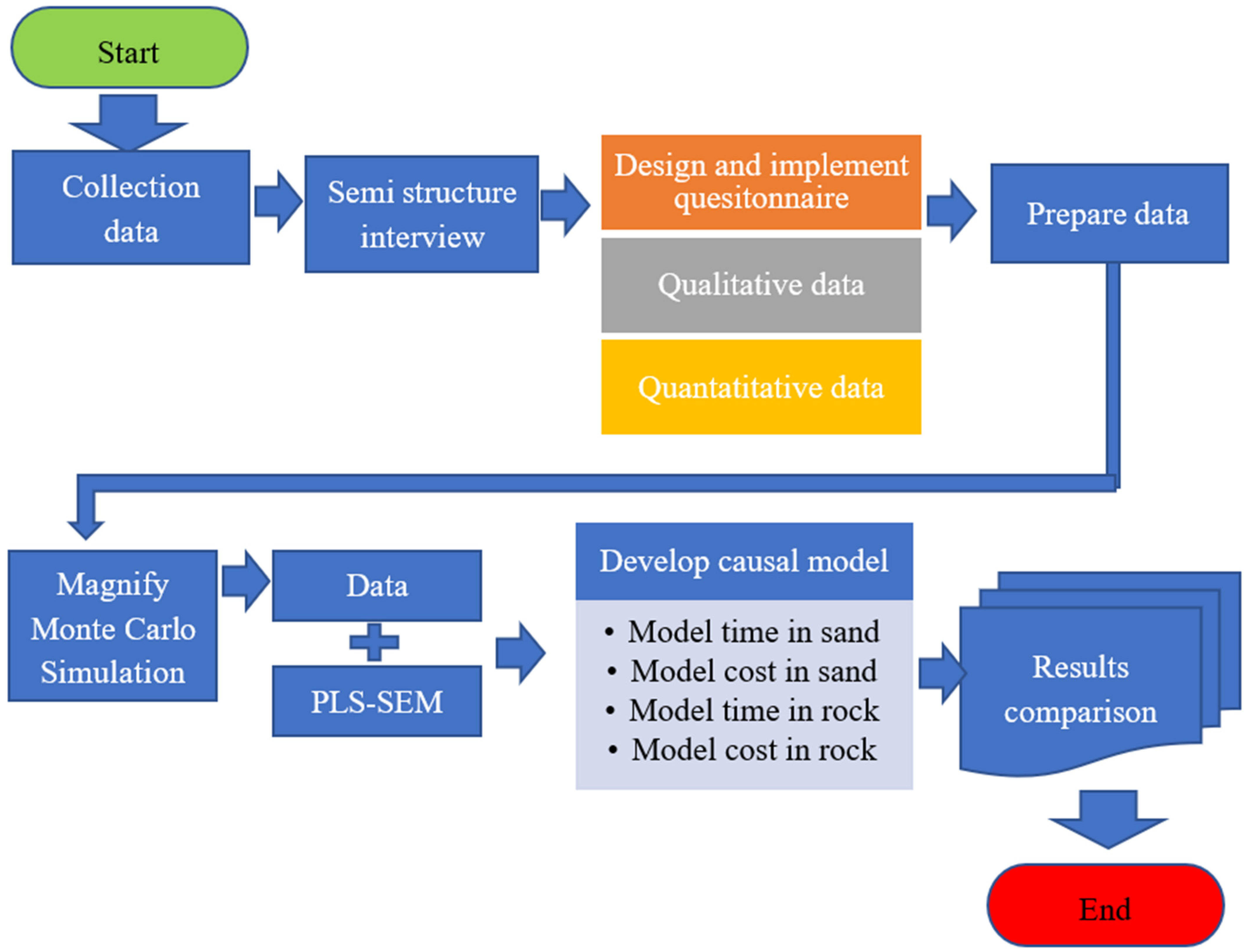
3. Research Methodology

This study adopted a cross-sectional, questionnaire-based survey to evaluate risk factors relating to pile construction projects in the KSA. The study methodology consisted of (1) conducting semi-structured interviews, (2) designing and implementing a survey, (3) preparing data, (4) magnifying data, (5) developing a time and cost risk interdependency model using the PLS-SEM, and (6) comparing the results with previous studies. Figure 1 presents the adopted research methodology. The purpose of the collection of data was to gather all the pile installation risks in the literature. Then, five pile construction experts with experience in bored pile installation reviewed and examined the collected risk factors via semi-structured interviews. The pile construction experts added any risk factors missing from the first list of risk factors. After finalizing the risks that can influence pile construction in the KSA, the questionnaire was designed and distributed to the twelve experts to measure the degree of probability and the impact of the risks using a five-point Likert scale. Descriptions of the questionnaire data were prepared to digitize these data. The data were then magnified using a Monte Carlo simulation. The magnified data were then utilized to develop time and cost risk interdependencies for two terrain conditions (sand and rock). Lastly, the results of the interdependencies were compared with the results in the literature. The following subsections provide an overview of the adopted research approach.

3.1. Data Collection

The time and cost risks that may influence the construction of a pile foundation were collected from the literature, published papers, reports, and books. The review process resulted in 60 risk factors which were classified as external risks, design risks, management risks, construction risks, subcontractor risks, equipment risks, political and governmental risks, economic risks, owner-generated risks, and site risks.

3.2. Semi-Structured Interviews

The objective of conducting the semi-structured interviews was to review the risks collected from the literature and examine the suitability of pile installation in the Saudi construction industry. The semi-structured interviews were conducted with five pile construction experts. The experts agreed with 50 out of the 60 of the collected risks. The experts added another risk factor related to the equipment utilized in the pile-installing activity. The final list of 53 risk factors, along with the classifications (i.e., risk groups), are reported in Table 1. In Table 1, each risk factor was assigned a symbol associated with its risk group. The experts’ responses in the first stage identified risks that may occur and affect the construction of piles in the KSA. They agreed that the presented risks occur more often in the field. The experts also recommended adding some risks such as “The distance between the pile and the adjacent pile, DR7”, “The nature of the project (piles for the foundations of a building and a bridge, or piles supporting the excavation walls), DR8”, “The number of equipment on site, EQR8”, and “Drilling machine size, EQR9”. These risks were added to the appropriate groups, as shown in Table 2.

3.3. Designing and Conducting the Survey of Experts

After gathering the risk data, the questionnaire survey for the experts was designed based on the risk factors collected from the literature and the expert interviews. The questionnaire was administered in two sequential phases. The first questionnaire was used to check whether a risk has an influence on or does not influence the cost and time of pile construction. This questionnaire allowed for the collection of additional risks that may occur in the KSA’s pile construction industry from the experts. After incorporating the other risks into the appropriate groups, the second questionnaire survey, which consisted of 53 questions representing the qualitative questions, was administered to determine the degree of the probability of occurrence (P) and the degree of impact (I) on the two issues (the time and cost of pile installation) per question, using five Likert scales. The Likert scales, ranging from 1 to 5, represented very low, low, moderate, high, and very high, respectively. It is worth noting that the questionnaire designed in two stages was designed in Arabic to improve its ease of accessibility and understandability for the participants. Two quantitative questions related to the time and cost of the construction of a single pile foundation were added to link the quantitative and qualitative analyses. Hence, each respondent provided 53 qualitative responses and two quantitative responses. The questionnaire survey was administered via electronic questionnaires, phone calls, and contacting and emailing 12 pile construction experts with at least ten years of experience in the pile construction industry in three sequential stages. The experts consisted of two academics, an engineer manager, and nine engineers who supervised the implementation of pile foundations. The questionnaire was then implemented as the second stage.

3.4. Data Preparation

Data preparation was conducted with the aim of changing or converting the descriptive values of the data questionnaire, represented by a five-point Likert scale scoring the degree of impact and its occurring probability, into numerical values to use these data as inputs for the PLS-SEM. The aim was achieved by replacing the five-point scale with its corresponding normalized values, as shown in Table 3. For each respondent and risk (the response to a question), the P and I were normalized using the maximum value of the Likert scale (5). Then, the risk score (RS) of the ith risk was computed by multiplying the degree of probability of the ith risk P i with the degree impact of the ith risk I i , as shown in Equation (1).
R S i = P i × I i
The RS data represent the qualitative data. Therefore, the RS matrix included 12 participants × 53 risks.
On the other hand, the quantitative data consist of the time and cost of the installation of a bored pile with a diameter of 1 m and a length of 20.0 m in sand, rock. To obtain the appropriate values of the time and cost of constructing the pile, the following limitations were considered in this study: the diameter of the pile is one meter, and the depth of the pile is twenty meters. Then, the third stage was performed through phone calls and by providing explanations to each expert. The experts were asked: What is the type of ground condition (rock, clay, or sand)? What is the drilling rate in an hour? How much is the total cost of constructing the pile per meter? Based on the answers to the previous questions, the time and cost of constructing a single pile were determined. Therefore, the three ground conditions were assigned as input data beside the 53 risks. Therefore, each participant provided the degree of probability and impact of the 53 risks and estimated the average time and cost of constructing a pile in common terrain conditions (sand, rock, and clay). The time (Ti) and cost (Ci) data were normalized using Equations (2) and (3), respectively.
T i ¯ = T i T m i n T m a x T m i n
C i ¯ = C i C m i n C m a x C m i n
where T m i n and C m i n are the minimum values of time and cost, respectively, and T m a x and C m a x are the maximum time and cost, respectively.

3.5. Magnifying and Normalizing the Data Using a Monte Carlo Simulation

A Monte Carlo simulation was utilized to predict the probability of different outcomes in a process that cannot be easily predicted due to the intervention of random variables. This technique models the stochastic behavior of risk occurrence and generates numerous possible risk scenarios through simulation. It is a method utilized to understand the impact of risk and uncertainty. A Monte Carlo simulation generates probabilities using random numbers to emulate possible outcomes. This type of simulation is widely used as an analysis tool in risk management applications, especially when the data required are relatively small [41]. The process of using a Monte Carlo simulation involves defining variables and assigning a probability distribution. The essential variables are identified. These variables can be deterministic (such as the mean and standard deviation) or probabilistic (with uncertain or random values). The probability distribution that represents the range of possible values and their likelihoods is assigned. This study integrated a Monte Carlo simulation with a PLS-SEM to increase the necessary data.
The results of the simulation were utilized as the input for the PLS-SEM. The data presented in Table A1 (in the Appendix A) were magnified using a Monte Carlo simulation in Excel software. Each risk’s mean and standard deviation were utilized to achieve the simulation. In addition, the distribution type was set as a normal distribution. There were 350 of data generated for the time and cost of the two terrain conditions (sand and rock). Because the minimum number of data used in the PLS-SEM is ten times the number of the paths that may be created, the minimum number of paths was set to ten (the number of directed paths from the groups to the cost or time of pile installation). Therefore, the number of items of data required for the PLS-SEM was 100.

3.6. Developing an Interdependency Model Using a PLS-SEM

The subsection provides information on PLS-SEMs and the procedures of constructing causal models based on data generated via a Monte Carlo simulation.

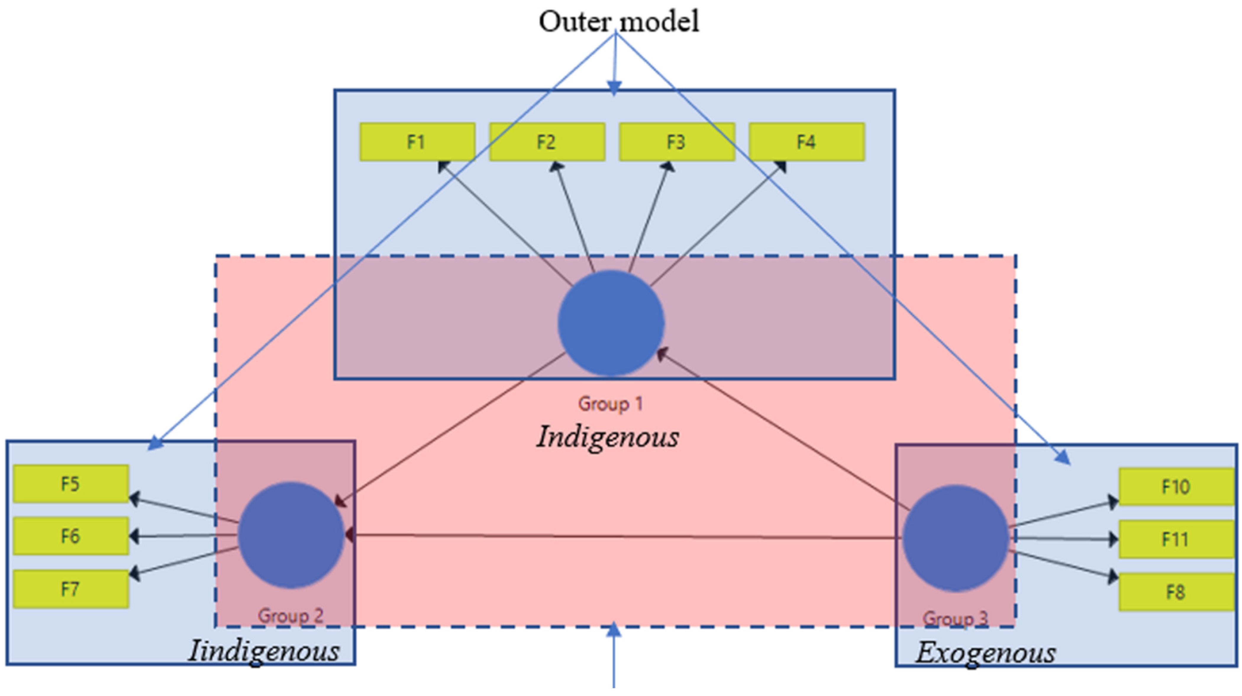
3.6.1. Information on the Components of a PLS-SEM

The purpose of this paper is to examine the influence of interdependencies and identify the crucial factors impacting the time and cost of pile installation in rock and sand conditions. A PLS-SEM can recognize the interrelationships among factors by conducting hypothesis assumptions among factors [42]. A PLS-SEM model includes outer and inner models. The outer model studies the relationships between the group (latent/construct) and its indicators, which are classified as reflective (arrows from indicators to their group) or informative indicators (arrows from the group to its indicators) [42]. The inner model represents the interrelationships among the groups, classified as exogenous and indigenous. The exogenous group influences other groups, as shown in Figure 2. At the same time, the indigenous group is affected by one or more groups. Figure 2 presents the general components of a PLS-SEM model.

Outer Model Assessment

The assessment of the outer model aims to omit the factors unrelated to the group; this can be achieved by assessing the construct and reliability validity (Cronbach’s alpha, composite reliability, and the average variance extracted) and discriminant validity (Fronell–Larcker criteria and cross-loading). The construct and reliability validity are used to measure Cronbach’s alpha (α), the composite reliability (CMR), and the average variance extracted (AVE) of the group with acceptable-level values of 0.70, 0.70, and 0.50, respectively [43]. They can be computed based on the outer loading of the group’s indicators ( λ i ) , as shown in Equations (4)–(6) [42], respectively.
α = K K 1 1 i = 1 K S i 2 S t 2
C R = i = 1 K λ i 2 i = 1 K λ i 2 + var ( e i )
A V E = i = 1 K λ i 2 i = 1 K λ i 2 + var ( e i )
where K is the number of the factors, s i 2 is the variance of the ith factor, s t 2 is the total variance, λ i is the standardized loading value of the ith factor, and   V a r e i is the error variance of the ith factor. The values of α and CR should exceed 0.7. In addition, the AVE should be more than 0.5. When one of the three-construct coefficient (α, CR, and AVE) values does not satisfy the threshold value, the impact of the elimination of each factor on the unsatisfied coefficient is studied. For example, if eliminating the ith factor leads to an increase in the value of the unsatisfied factor, this factor should be deleted unless the factor should remain. The discriminant validity can be measured using the Fronell–Larcker criteria among the group and cross-loading for the factors and groups [43]. Due to its simplified usage, the SmartPLS software was utilized in this study to carry out the contract and discriminant validity assessments. The outer (the relationship of groups with their factors) and inner models (the relationships among groups) are shown in Figure 2.

Inner Model Assessment

The primary purpose of the inner model assessments, which are performed after carrying out the outer model assessments, is to examine the hypothesis relationships and determine the model’s accuracy. These assessments include a hypothesis relationship test, predictive relevance, and a fitness model (determination coefficients). This assessment model can be achieved by examining the relationship between two latent groups by determining the b coefficient or p-value. These coefficients and values indicate whether the connection exists or not. Refer to the reference for more details on calculating the b and p [42]. If p is less than 10%, then the alternative hypothesis (b ≠ 0; there was a relationship between the two latent groups) is accepted. Otherwise, the null hypothesis (b = 0; no relationship between the two latent groups) is accepted.

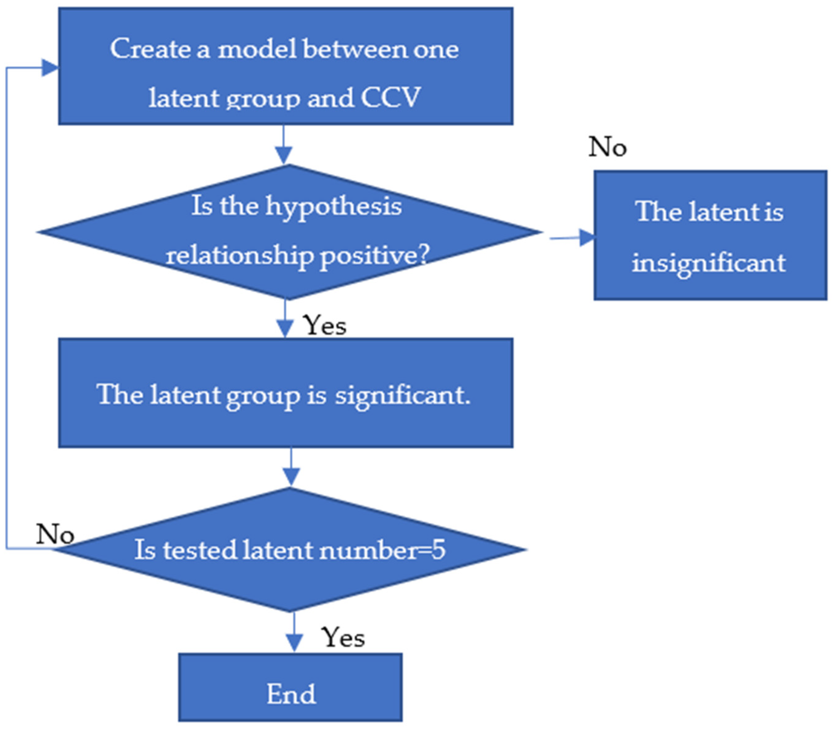
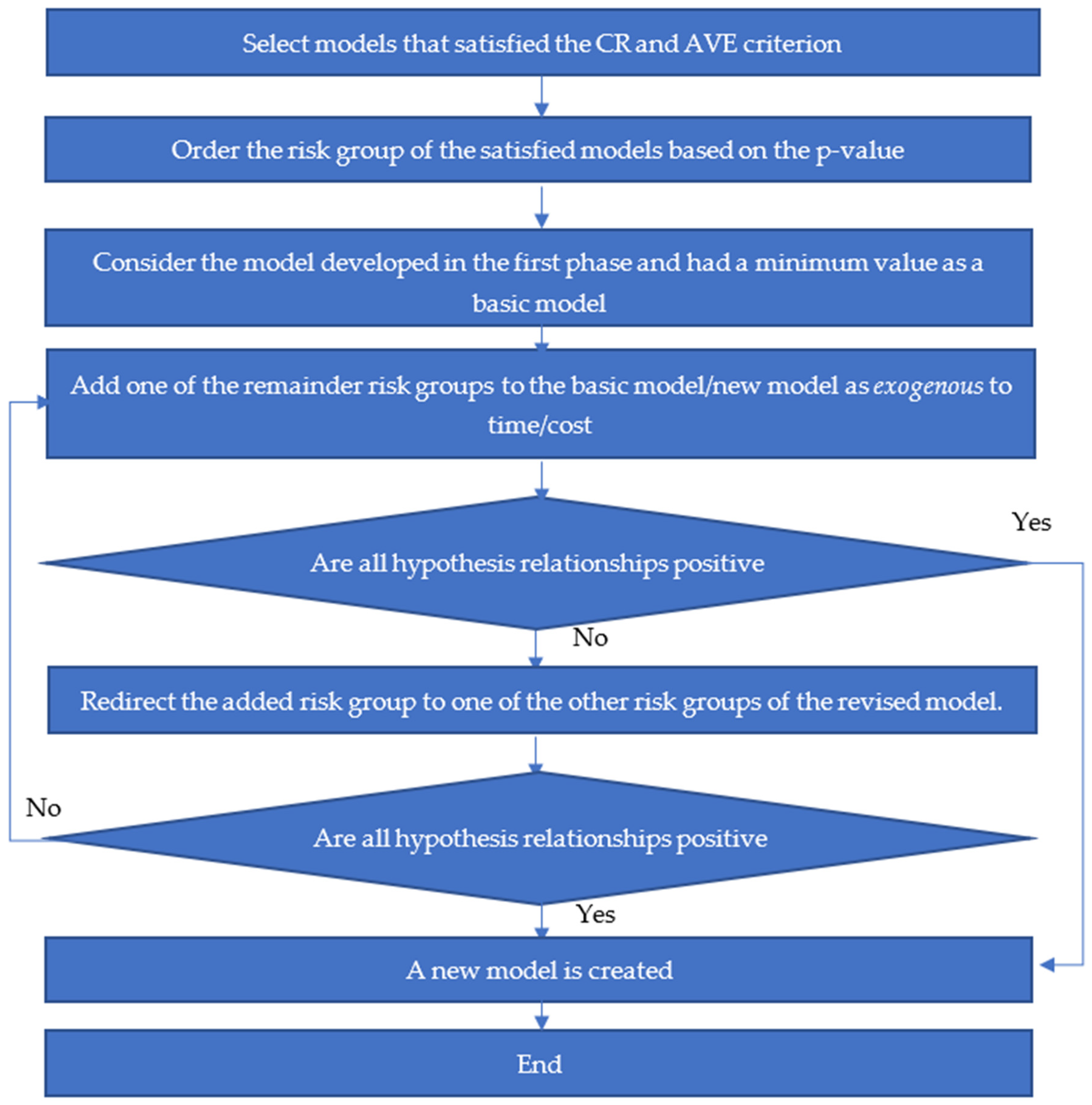
3.6.2. Establishing the Interdependency Model

This subsection explains the procedures and steps to creating the four interdependency models. These models represent the model’s time for pile installation in the sand ( M o d e l s a n d t i m e ), the model’s cost of pile installation in sand ( M o d e l s a n d c o s t ), the model’s time for pile installation in rock ( M o d e l r o c k t i m e ), and the model’s cost of pile installation in rock ( M o d e l r o c k c o s t ). The model development processes were based on the data generated by the Monte Carlo simulation. Therefore, there were four data sets (one for each model). The procedures were divided in sequence into two phases, as described below.

Phase One: Identify the Significant Groups

This phase aims to distinguish the significant groups from the insignificant groups. The following steps were performed to achieve the purpose of the first stage.
Step 1: Ten models were created; each model consisted of one exogenous group (ER, DR, MR, CR, SCR, EQR, PGRE, ECR, OGR, or SR) and one indigenous group (time or cost).
Step 2: The outer model was assessed for each model regarding construct and reliability validity.
Step 3: If the exogenous group of the model was satisfied, especially for the CR and AVE, the groups were considered significant. Otherwise, the group was considered insignificant.
Step 4: The hypothesis relationship of each model was examined.
These steps are depicted in Figure 3.
The CR and AVE of the exogenous group depended on the outer loading of its factors. They were assessed several times by studying the omission of one or more factors that had a lower outer loading on the CR and AVE of the group. These steps resemble the studies conducted by Alsugair [36] and Hair and Sarstedt [42], which can be referred to for more information.
Table 4 and Table 5 show the CMR and AVE of ten models for the time and cost of installing a pile in the sand, respectively. ER and ECR are insignificant risk groups for the time and cost of pile installation in sand. However, DR, CR, EQR, and SR are significant risk groups for time and cost. In addition, MR and OGR are significant risk groups for time and cost, respectively. At the same time, Table 6 and Table 7 show the CMR and AVE of ten models for time and cost of installing a pile in rock, respectively. The insignificant risk groups for the time and cost of installing a pile in rock are ER, MR, and PGR.
On the other hand, the common significant risk groups for cost and time are DR, CE, OGR, and SR. In addition, EQR and SCR are considerable risk groups for time and cost, respectively. Table 4, Table 5, Table 6 and Table 7 also display the significant factors in each group.

Phase Two: Merge the Significant Risk Groups into One Model

This method establishes the interdependency network of the time and cost of installing a pile in the two terrain conditions. The steps of the second phase were as follows:
Step 1: Models that satisfy the CR and AVE were selected.
Step 2: The satisfying models were ordered based on the p-values.
Step 3: The risk group was ranked based on the operation order in Step 1.
Step 4: The model with a minimum p-value was considered a basic model.
Step 5: Another risk group (second-order risk group) was added to the basic model as an exogenous group to the time or cost group. A revised model was created.
Step 6: The two-hypothesis relationship of the revised model was examined.
Step 6.1: If the p-value hypothesis was smaller than 0.10 (with a corresponding confidence level of 10%), the revised model was changed to the newly developed model.
Step 6.2: Otherwise, the added risk group was redirected to one of the other risk groups of the revised model.
Step 6.3: All hypothesis relationships were examined.
Step 6.3.1: If the p-value of all hypotheses was smaller than 0.10, the new model was developed.
Step 6.3.2: Otherwise, the added risk group was omitted.
Step 7: Steps 1 to 6.3 were repeated for the remainder of the risk groups.
The second phase step is summarized in the flowchart shown in Figure 4.

4. Results and Discussion

Risk interdependency models for pile installation in sand and rock terrain conditions are displayed to assess these risks well.

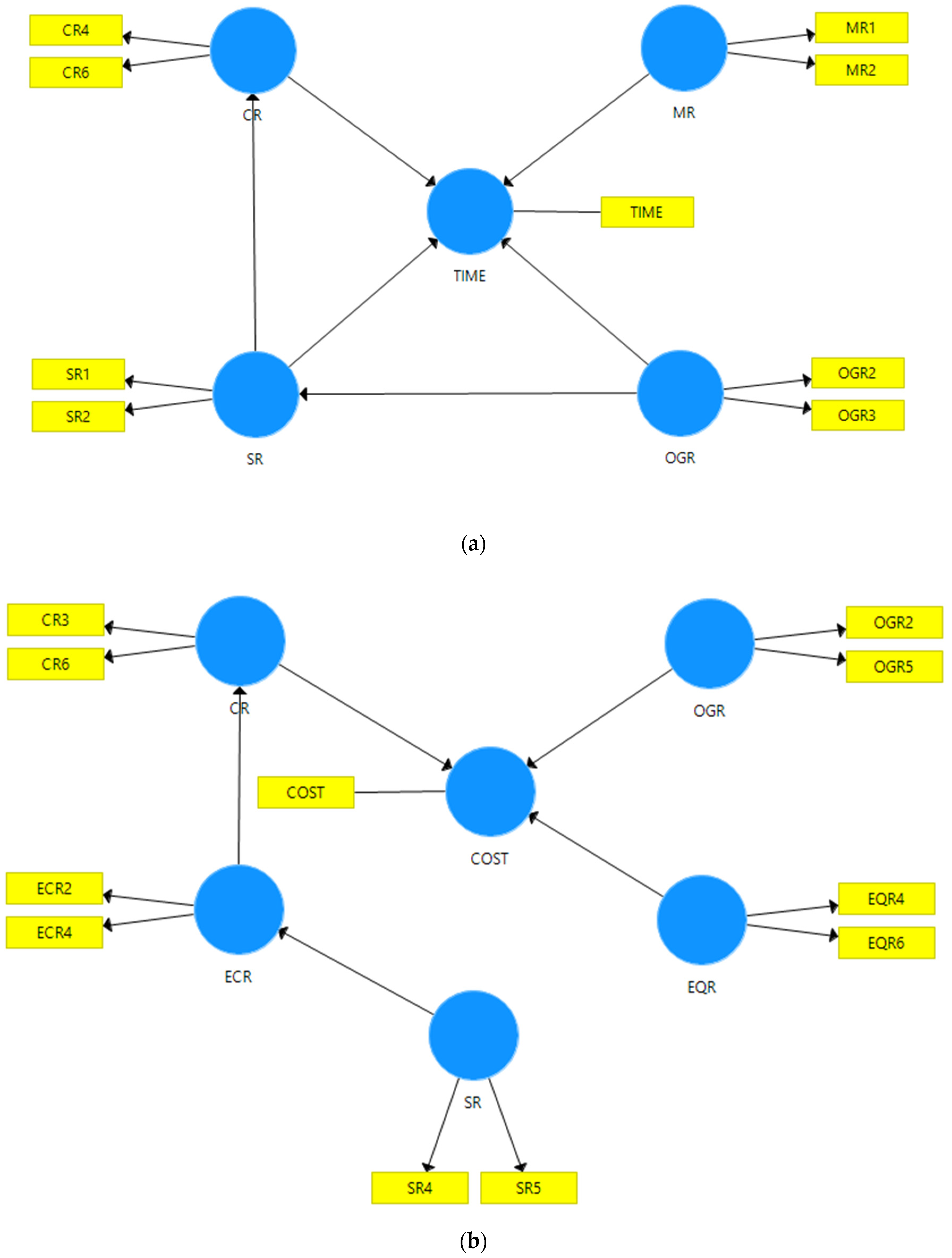
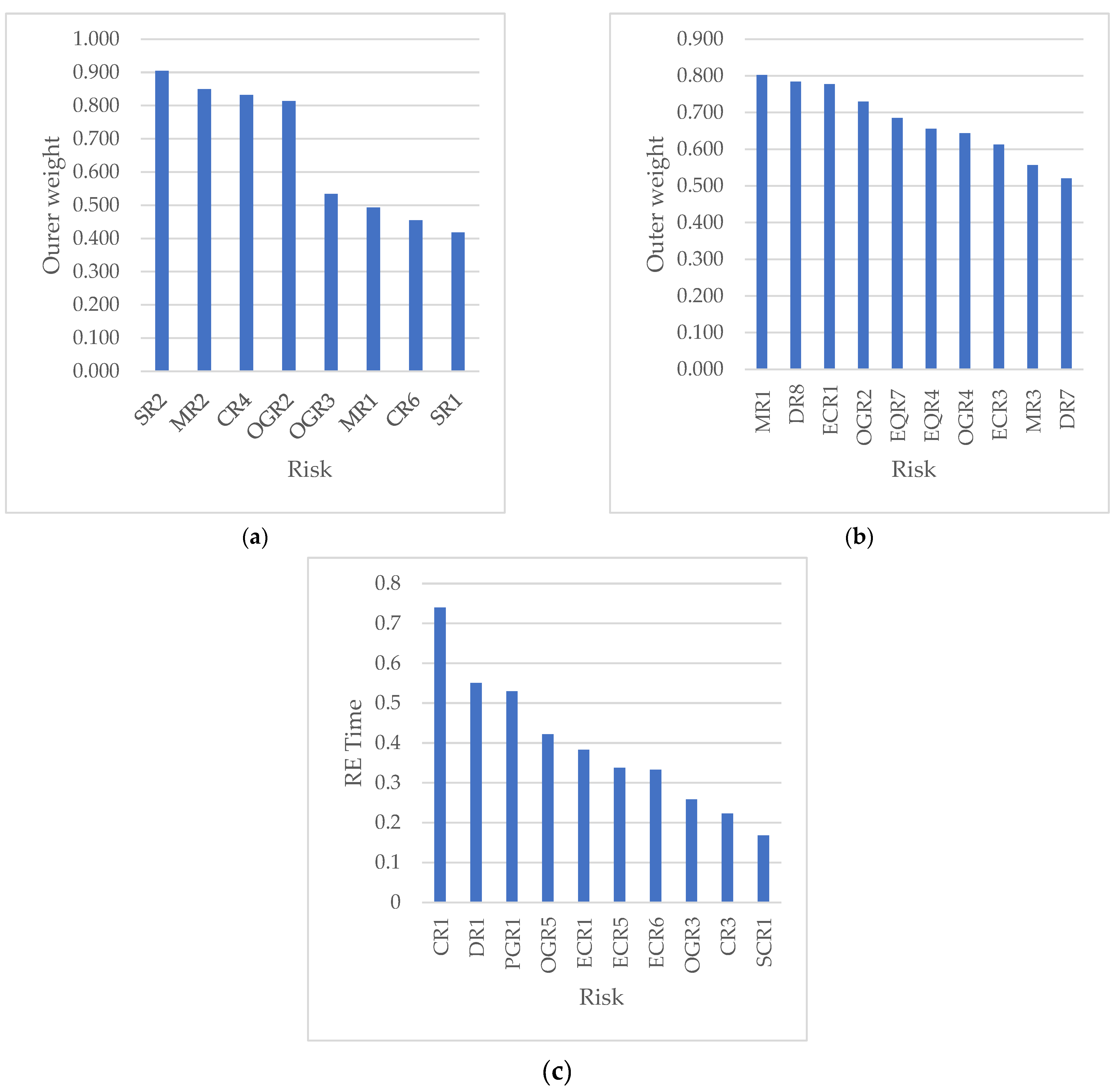
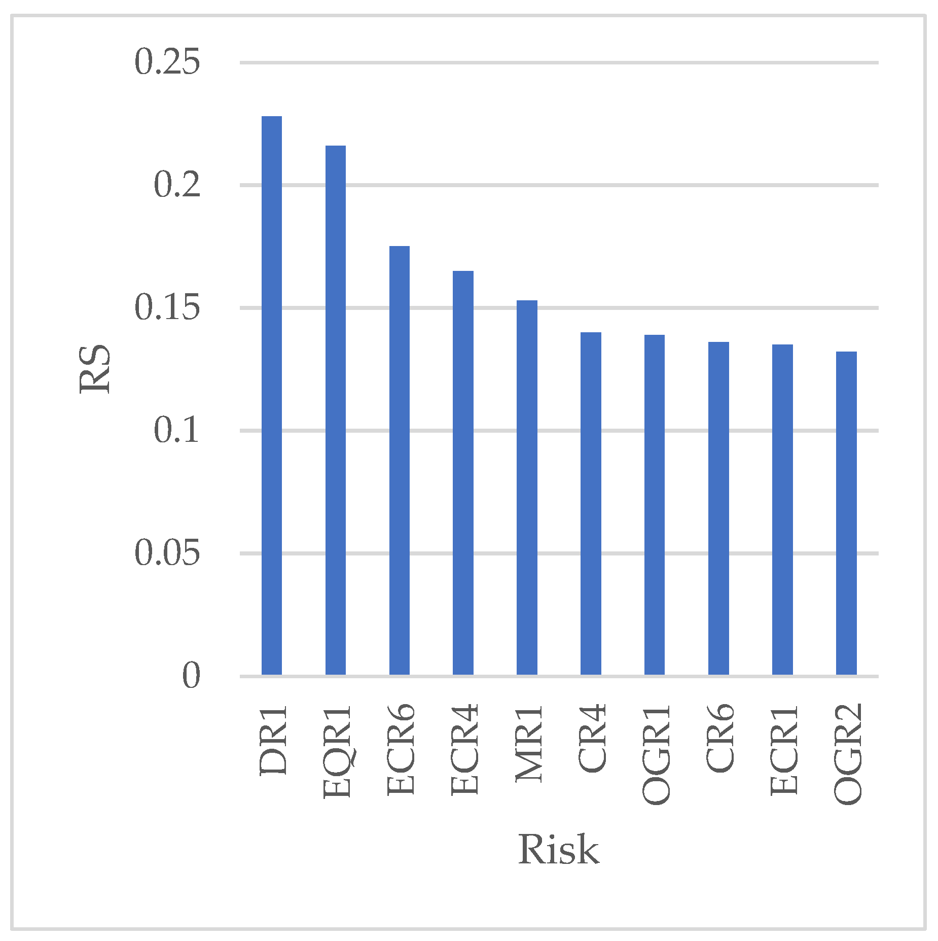
4.1. Risk Interdependency Model in Sand

The CMR and AVE of the significant risk groups for the time and cost of pile installation are presented in Table 8. The common risk groups shared in the time and cost were CR, OGR, and SR. However, MR is a significant risk group for time. ECR and EQR, on the other hand, each play a crucial role in the cost. The CMR value of some risk groups is slightly lower than the acceptable level (0.7). Hence, the models suffered slight violations of reliability. The AVE values of all time and cost risk groups are higher than the threshold value (0.5). In addition, Table 9 shows the discriminant validity in terms of the Fronell–Larcker criterion. The results showed that the square root of the AVE of the risks group, shown in the diagonal element of Table 9, is higher than the correlation coefficient between the two risk groups. Therefore, the time and cost model satisfied the Fronell–Larcker criterion.
As for the cross-loading criterion, Table 10 shows the cross-loading values of significant risks for different risk groups of time and cost. The related risk values to the risk groups shall be higher than the value of the unrelated risk. For example, the cross-loading value of CR4 and CR6 to the CR were 0.893 and 0.565 (shown in red writing in Table 10), respectively. These values are higher than the unrelated cross-loading risks to CR (MR1, MR2, OGR2, OGR3, SR1, and SR2), shown in Table 10. Therefore, the time and cost models were satisfied with respect to discriminant validity.
Figure 5 shows the interrelationships among the risk groups with the significant risks of pile installation with respect to time (Figure 5a) and cost (Figure 5b). The model considered the qualitative and quantitative analyses, as previously illustrated in the Research Methodology section. The significant risks of CR, MR, OGR, and SR are (CR4, CR6), (MR1, MR2), (OGR2, OGR3), and (SR1, SR2), respectively. Figure 5 also presents the interrelationships among the risk groups for the time and cost of pile installation. The statistical test results of these interrelationships (paths) in terms of b coefficients, t-values, and the corresponding p-values are shown in Table 11. The p-values are less than 0.1 (a confidence level of 90%).
The CR and MR directly influence the time needed to install a pile for the time risk interdependency model. At the same time, the OGR and SR affect the time needed for pile installation directly and indirectly through SR and CR, respectively. Financial difficulties (OGR2) may have a detrimental influence on the investigation samples that should cover the entire area of the structure (SR1). In addition, the results indicate that site risks influence safety issues (CR4) and site survey errors (CR6). For instance, the soil type (SR1) and the number of investigation samples impact the safety with respect to bearing failure.
Regarding the risk interdependency model of the cost of pile installation, CR, OGR, and ECR directly affect the cost. On the other hand, SR and ECR indirectly affect the cost through CR. For example, considering space risks at the construction site (SR4) caused by crowded equipment, leads to issues with site handling (CR6). In addition, SR4 leads to an increase in working pressure on workers and, as a result, labor conflicts and disputes (CR4). Furthermore, SR has an impact on the improper maintenance of equipment. Moreover, preexisting site infrastructures (SR4), such as buried power and communication cables, affect site handling (CR6).

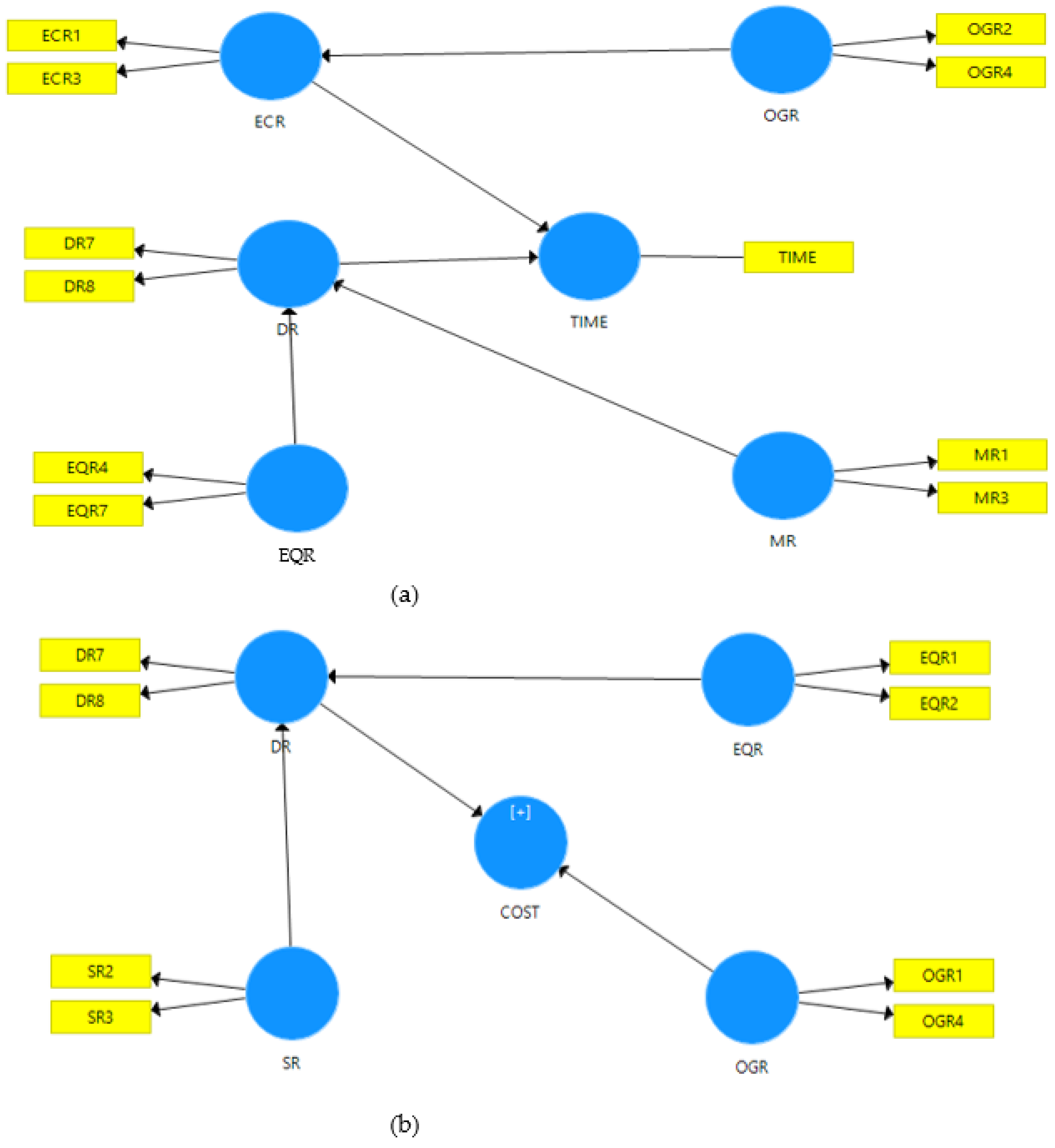
4.2. Risk Interdependency Model in Rock

Table 12 displays the CMR and AVE of the primary risk groups for the time and cost pile installation in rock. DR, EQR, and OGR were the common risk groups that shared time and cost. On the other hand, MR and ECR represent significant risk groups. Moreover, SR has a considerable effect on the cost. Some risk groups, such as ECR, MR for time, and EQR for cost, have CMR values that are marginally below the permitted range (0.7). As a result, the models’ dependability was somewhat violated. All time and cost risk categories have AVE values higher than the criterion (0.5).
Table 13 displays the discriminant validity according to the Fronell–Larcker criterion. The findings reveal that the square root of the AVE for the risk group, shown in the diagonal element of Table 13, is greater than the correlation coefficient between two separate risk groups. The Fronell–Larcker criteria were met for the time and cost model. The cross-loading values of crucial risks for various risk groups in terms of time and cost are shown in Table 14, the cross-loading criterion. The risk groups’ associated risk values must be greater than the unrelated values. As a result, the time and cost model’s discriminant validity requirements were met.
Figure 6 depicts the interactions between the risk groups and the significant risks associated with installing piles in rock for time (Figure 6a) and cost (Figure 6b). The risk groups most relevant to time are (DR7, DR8), (ECR1, ECR3), (EQR4, EQR7), (MR1, MR3), and (OGR1, OGR2) are the respective major risks for DR, ECR, EQR, MR, and OGR. The substantial cost risks for DR, EQR, OGR, and SR are, respectively, (DR7, DR8), (EQR1, EQR2), (OGR1, OGR4), and (SR2, SR3). The linkages between the risk groups for the installation of a pile in terms of time and cost are also shown in Figure 6. Table 15 displays the results of these interrelationships’ statistical tests regarding b coefficients, t values, and the accompanying p values. The p-values were less than 0.1.
The results of the time model indicate that risks regarding a lack of quality management (MR7), such as planning, assurance, and control, play a role in the distance between the pile and the adjacent pile (DR7) and the length and diameter of the concrete pile (DR8). Moreover, an owner’s ultra-standards (OGR4) may lead to a lack of funds or a lack of cash flow (ECR2) and improper maintenance (ECR2). There is a relationship between the risk of the size of the withdrawn unit (EQR7) and the risk of the length and diameter of the pile concrete (DR8).
Regarding the risk interdependency model of the cost of pile installation, DR and OGR directly affect the cost. On the other hand, the SR and EQR risk groups indirectly affect the cost through DR. For example, the risk of soil type (SR2) plays an essential role in the risk of the distance between the pile and an adjacent pile (DR7) and on the length and diameter of the pile concrete (DR8). In addition, there is a risk due to the size limitation of the equipment (SR3) on the length and diameter of the concrete pile (DR8).
The rankings of the significant time risks for pile installation in sand and rock were compared and are shown in Figure 7a,b, respectively. Management risks are essential to the time needed to construct a pile in sand via MR1 and MR2, while MR1 and MR3 are crucial time risks for constructing a pile in rock. In addition, the most relevant risk groups for sand are construction risks (CR4 and CR6) and owner-generated risks (OGR2 and OGR3), as shown in Figure 7a. On the other hand, the essential risk groups for rock are economic risks (ECR1, ECR7, and ECR3) and owner-generated risks (OGR2 and OGR4), as shown in Figure 7b. Based on these risk groups, the results provided by the time risk interdependency model in rock agreed with the results of the study by Al-Gahtani and Alsanabani [16], in which OGR, ECR, and DR are the significant risk groups for pile installation time, as shown in Figure 7c.
Figure 8a,b present the rankings of the significant cost risks for pile installation in sand and rock, respectively. The three considerable risk groups for pile installation in sand were economic, equipment, and owner-generated risks, with of ECR4, EQR2, and OGR4, respectively, as shown in Figure 8a. On the other hand, the three crucial cost risk groups for installing a pile in rock are equipment, owner-generated, and design risks, with EQR1, OGR4, and DR8, respectively, as shown in Figure 8b. The results of Al-Gahtani and Alsanabani [15] indicated that the owner-generated and design risk groups are the essential risk groups for the costs of pile installation (DR1 and OGR5), as shown in Figure 8c. These results align with the ranking of the cost risk interdependency in rock, as shown in Figure 8b.
Hosny et al. [5] utilized study results to compare risk rankings. The top ten risks of their study are shown in Figure 9. The results indicate that the “Improper and insufficient assessment of soil, DR1” had the highest risk for the cost and time needed to construct a pile, which agreed with the results of this paper. Their results also indicate that ECR1 (lack of funds: a lack of cash flow from the contractor) and ECR6 (foreign exchange risks: unstable exchange rates, transfer restrictions, and supply and demand balance) hazards are among the top ten threats in the piling industry, which is consistent with the results reached in this study, as shown in Figure 7a,c. However, the rest of the ten factors are quite different due to the differences in the method used, as the method used in the research by Hosny et al. [5] was a descriptive analysis. In contrast, the technique used in this study is a mixture of descriptive and quantitative analyses. The difference may also be attributable to the different market conditions and environments between the KSA and Egypt.

5. Conclusions

This study identified and examined the interdependencies among the time and cost risks of pile installation in the KSA’s construction industry. The research methodology involved several steps. Firstly, data were collected to gather all the pile installation risks in the literature. Then, the listed risks were reviewed and examined, and pile construction experts assessed other risks via semi-structured interviews. After obtaining the risks that may influence pile construction in the KSA, a survey was designed and distributed to the twelve experts to measure the degree of probability and impact of each of the risks using a five-point Likert scale. The questionnaire data were prepared. The data were then magnified using a Monte Carlo simulation. The elaborated data were then utilized to develop time and cost risk interdependencies for two terrain conditions (sand and rock). The results of the interdependencies were compared with the literature.
This study’s findings show that construction risk indirectly impacts the time and cost needed to install a pile time and cost in sand due to site and economic risks through design risks. Moreover, site hazards and equipment risks indirectly affect the cost of installing piles in rock. The significant risk groups for the time needed to install a pile in the sand are construction risks (safety issues, survey errors, and site handling mistakes), management risks (poor communication between project stakeholders and poor staff efficiency), owner-generated risks (unqualified owner representatives and the delay or refusal of compensation to the contractor), and site risks (when the investigation samples do not cover the entire study area and soil type). The crucial time risk groups for constructing a pile in rock are design risks (the distance between the pile and the adjacent pile and the nature of the project), economic risks (a lack of funds: a lack of cash flow from the contractor, and delays in the delivery of services and spare parts), equipment risks (a delay in and/or failure of logistics services and the size of the withdrawal units), management risks (poor communication between project stakeholders and a lack of quality management) and owner-generated risks (failure to finance the project and unqualified owner representatives). The substantial cost risks of installing a pile in rock are the distance between the pile and an adjacent pile, the nature of the project, incidents with internal or external stakeholders, improper maintenance, failure to finance the project, an owner’s ultra-standard expectations and requirements, the soil type, and issues due to size limitations. These results aid the building industry in more efficiently assessing time and expense concerns. This paper is limited to bored piles in the construction stage. The paper did consider the mutual relationship between time delays and cost overruns.
Further studies are recommended to investigate the risks of the interdependency model using artificial intelligence (AI) or machine learning (ML). The paper was limited to a risk assessment of one type of pile: a bored pile. In addition, the types of sub-ground conditions were limited to sand and rock.

6. Recommendation for Further Studies

Further future studies are recommended to extend this study for driven and flight auger piles. The authors recommend applying the study methodology to consider the environmental risks for pile-driven offshore structures.

Author Contributions

Conceptualization, A.S.A. and K.S.A.-G.; data curation, N.M.A. and K.S.A.-G.; formal analysis, N.M.A. and K.S.A.-G.; funding acquisition, A.A. and K.S.A.-G.; investigation, A.S.A., N.M.A. and K.S.A.-G.; methodology, N.M.A., K.S.A.-G. and A.A.; project administration, A.S.A., K.S.A.-G. and A.S.A.; resources, A.S.A. and K.S.A.-G.; software, N.M.A.; supervision, A.S.A. and K.S.A.-G.; validation, N.M.A., K.S.A.-G. and A.S.A.; visualization, A.S.A., N.M.A., K.S.A.-G. and A.S.A.; Writing—original draft preparation, N.M.A. and K.S.A.-G.; Writing—review and editing, A.S.A., N.M.A., K.S.A.-G. and A.A. All authors have read and agreed to the published version of the manuscript.

Funding

The authors extend their appreciation to the Deputyship for Research and Innovation, Ministry of Education in Saudi Arabia for funding this research work through the project no. (IFKSUOR3-380-3).

Institutional Review Board Statement

Not applicable.

Informed Consent Statement

Not applicable.

Data Availability Statement

The data in this paper were taken from other studies and experts. The raw data supporting the findings of this paper are available upon request from the corresponding author.

Conflicts of Interest

The authors declare no conflict of interest.

Appendix A

Table A1. Risk score (RS = P*I) of the 53 risks with the cost and time of pile construction (second stage).
ER1ER2DR1DR2DR3DR4DR5DR6DR7DR8MR1MR2MR3
Expert 10.250.090.350.490.250.350.210.350.250.350.350.490.49
Expert 20.350.350.450.210.350.270.210.350.090.350.210.450.27
Expert 30.090.270.050.010.010.350.270.090.150.050.210.270.35
Expert 40.150.350.210.090.150.250.350.350.350.350.350.350.35
Expert 50.210.150.210.030.350.250.350.090.350.050.030.350.15
Expert 60.210.250.490.150.250.350.210.250.250.250.210.210.35
Expert 70.090.350.810.630.350.630.630.810.810.630.630.630.81
Expert 80.010.070.270.050.250.030.050.050.090.090.030.050.15
Expert 90.250.150.450.090.250.210.490.210.150.150.090.350.25
Expert 100.090.490.250.090.490.490.490.250.250.250.090.090.09
Expert 110.150.150.350.150.490.250.150.010.250.210.810.010.01
Expert 120.010.010.250.090.090.010.090.250.250.010.250.490.49
CR1CR2CR3CR4CR5CR6CR7CR8CR9CR10SCR1SCR2SCR3
Expert 10.350.150.090.090.250.350.450.350.350.450.250.150.09
Expert 20.450.630.350.630.250.350.210.210.350.450.350.450.45
Expert 30.150.350.350.450.090.350.090.150.270.030.250.630.25
Expert 40.210.250.250.350.450.350.630.150.630.350.150.630.25
Expert 50.350.490.150.350.350.090.210.030.210.210.350.050.21
Expert 60.050.250.090.210.250.250.010.090.250.150.090.350.25
Expert 70.450.490.350.490.490.450.350.350.630.450.350.490.35
Expert 80.050.050.030.050.090.070.090.090.050.030.050.030.09
Expert 90.210.150.450.150.090.210.150.150.150.210.250.090.09
Expert 100.350.250.250.250.250.090.090.090.250.250.250.150.25
Expert 110.490.090.350.810.810.630.150.090.810.490.810.810.63
Expert 120.250.090.250.490.090.090.090.250.490.090.250.010.25
ER1ER2ER3ER4ER5ER6ER7ER8ER9PGR1PGR2ECR1ECR2
Expert 10.150.150.090.090.150.090.090.250.090.150.090.350.15
Expert 20.210.350.450.450.450.210.210.450.150.450.350.450.35
Expert 30.150.210.630.350.270.090.210.450.450.090.090.630.35
Expert 40.250.150.150.150.250.150.250.490.350.630.250.450.25
Expert 50.030.010.030.350.350.210.150.210.150.350.050.350.03
Expert 60.250.250.350.250.250.150.350.350.150.270.350.350.25
Expert 70.350.350.490.630.450.490.490.630.630.210.490.490.49
Expert 80.030.090.030.050.050.030.030.250.250.090.090.150.09
Expert 90.090.350.030.090.150.150.150.150.150.150.090.350.35
Expert 100.250.250.250.090.250.090.090.090.090.250.250.250.09
Expert 110.350.810.010.010.350.250.250.010.350.490.490.810.81
Expert 120.250.250.090.090.090.250.250.090.250.250.250.090.09
ECR3ECR4ECR5ECR6OGR1OGR2OGR3OGR4OGR5
Expert 10.090.250.250.250.250.150.210.090.15
Expert 20.350.250.250.150.270.450.150.350.35
Expert 30.350.150.210.050.350.630.350.630.45
Expert 40.250.630.350.350.350.070.250.350.25
Expert 50.030.150.050.150.210.210.050.210.21
Expert 60.150.250.150.210.350.450.350.150.21
Expert 70.490.490.450.350.630.630.630.810.63
Expert 80.150.090.050.030.050.150.150.150.09
Expert 90.150.150.150.090.350.150.150.350.15
Expert 100.090.250.090.090.090.090.090.090.09
Expert 110.090.810.090.090.010.490.490.630.15
Expert 120.010.090.250.090.010.090.090.090.01
SR1SR2SR3SR4SR5Cost/pile (SAR)Duration/pile (hour)
Expert 10.250.630.150.090.090.170
Expert 20.450.450.250.250.450.280.04
Expert 30.250.350.270.150.150.080
Expert 40.150.630.350.150.250.130
Expert 50.210.350.350.150.3500.4
Expert 60.150.210.150.210.350.220.01
Expert 70.630.630.630.490.630.970.64
Expert 80.030.030.030.010.090.750.4
Expert 90.450.350.250.150.0911
Expert 100.250.250.090.090.090.90.28
Expert 110.150.150.490.490.350.880.82
Expert 120.250.250.250.250.250.840.73

References

  1. Report Store. “Saudi Arabia Construction Market Size, Trend Analysis by Sector (Commercial, Industrial, Infrastruc-ture, Energy and Utilities, Institutional and Residential) and Forecast, 2023–2027”. June 2023. Available online: https://www.globaldata.com/store/report/saudi-arabia-construction-market-analysis/#:~:text=The%20Saudi%20Arabia%20construction%20market,Vision%202030'%20economic%20diversification%20plan (accessed on 4 April 2023).
  2. Mordor Intelligence. Saudi Arabia Construction Market—Growth, Trends, COVID-19 Impact, and Forecasts (2023–2028). Available online: https://www.mordorintelligence.com/industry-reports/saudi-arabia-construction-market (accessed on 7 February 2023).
  3. World Economic Outlook Database; International Monetary Funds: Washington, DC, USA, 2023.
  4. Aziz, F.R. The Use of Simulation to Predict cfa Equipment Productivity; Alexandria University: Alexandria, Egypt, 2004. [Google Scholar]
  5. Hosny, H.E.; Ibrahim, A.H.; Fraig, R.F. Risk management framework for Continuous Flight Auger piles construction in Egypt. Alex. Eng. J. 2018, 57, 2667–2677. [Google Scholar] [CrossRef]
  6. Ehsan, N.; Mirza, E.; Alam, M.; Ishaqu, A. Notice of Retraction: Risk management in construction industry. In Proceedings of the 3rd International Conference on Computer Science and Information Technology, Chengdu, China, 9–11 July 2010. [Google Scholar]
  7. Choudhry, R.M.; Aslam, M.A.; Hinze, J.W.; Arain, F.M. Cost and Schedule Risk Analysis of Bridge Construction in Pakistan: Establishing Risk Guidelines. J. Constr. Eng. Manag. 2014, 140, 04014020. [Google Scholar] [CrossRef]
  8. Hosny, H.E.; Ibrahim, A.H.; Fraig, R.F. Cost analysis of continuous flight auger piles construction in Egypt. Alex. Eng. J. 2016, 55, 2709–2720. [Google Scholar] [CrossRef]
  9. Mata, P.; Silva, P.F.; Pinho, F.F.S. Risk Management of bored piling construction on sandy soils with real-time cost control. Infrastructures 2021, 6, 77. [Google Scholar] [CrossRef]
  10. Surenth, S.; Rajapakshe, R.M.P.P.V.; Muthumala, I.S.; Samarawickrama, M.N.C. Cost Forecasting Analysis on Bored and Cast-In-situ Piles in Sri Lanka: Case Study at Selected Pile Construction Sites in Colombo Metropolis Area. Eng. J. Inst. Eng. Sri Lanka 2019, 52, 57. [Google Scholar] [CrossRef]
  11. Zayed, T.M.; Halpin, D.W. Process versus Data Oriented Techniques in Pile Construction Productivity Assessment. J. Constr. Eng. Manag. 2004, 130, 490–499. [Google Scholar] [CrossRef]
  12. Zayed, T. Stochastic productivity assessment of continuous flight auger piles. Arch. Sci. Rev. 2009, 52, 17–27. [Google Scholar] [CrossRef]
  13. Zayed, T.M.; Halpin, D.W. Productivity and Cost Regression Models for Pile Construction. J. Constr. Eng. Manag. 2005, 131, 779–789. [Google Scholar] [CrossRef]
  14. Zayed, T.M.; Halpin, D.W. Pile Construction Productivity Assessment. J. Constr. Eng. Manag. 2005, 131, 705–714. [Google Scholar] [CrossRef]
  15. Al-Gahtani, K.; Alsanabani, N. Impact factors on time and cost in pile construction. Proc. Int. Struct. Eng. Constr. 2023, 10, 1. [Google Scholar] [CrossRef]
  16. Tsouvalas, A. Underwater noise emission due to offshore pile installation: A Review. Energies 2020, 13, 3037. [Google Scholar] [CrossRef]
  17. Juretzek, C.; Schmidt, B.; Boethling, M. Turning scientific knowledge into regulation: Effective measures for noise mitigation of pile driving. J. Mar. Sci. Eng. 2021, 9, 819. [Google Scholar] [CrossRef]
  18. White, D.; Finlay, T.; Bolton, M.; Bearss, G. Press-in piling: Ground vibration and noise during pile installation. In Deep Foundations 2002: An International Perspective on Theory, Design, Construction, and Performance; American Society of Civil Engineers: Reston, VA, USA, 2002; pp. 363–371. [Google Scholar]
  19. Zayed, T.M.; Halpin, D.W. Deterministic models for assessing productivity and cost of bored piles. Constr. Manag. Econ. 2005, 23, 531–543. [Google Scholar] [CrossRef]
  20. Mahamid, I.; Al-Ghonamy, A.; Aichouni, M. Factors affecting accuracy of pretender cost estimate: Studies of Saudi Arabia. Int. J. Appl. Eng. Res. 2014, 9, 21–36. [Google Scholar]
  21. Guan, L.; Abbasi, A.; Ryan, M.J. A simulation-based risk interdependency network model for project risk assessment. Decis. Support Syst. 2021, 148, 113602. [Google Scholar] [CrossRef]
  22. Wold, H. Model Construction and Evaluation When Theoretical Knowledge Is Scarce: Theory and Application of Partial Least Squares, In Evaluation of Econometric Models; Academic Press: Cambridge, MA, USA, 1980. [Google Scholar]
  23. Lohmöller, J.B.; Wold, H. Three-mode path models with latent variables and partial least squares (PLS) parameter estimation. In Proceedings of the European Meeting of the Psychometric Society, Groningen, The Netherlands, 19–21 June 1980. [Google Scholar]
  24. Hair, J.F.; Ringle, C.M.; Sarstedt, M. PLS-SEM: Indeed a Silver Bullet. J. Mark. Theory Pract. 2011, 19, 139–152. [Google Scholar] [CrossRef]
  25. Hair, J.F.; Ringle, C.M.; Sarstedt, M. Partial least squares structural equation modeling: Rigorous applications, better results and higher acceptance. Long Range Plann 2013, 46, 1–12. [Google Scholar] [CrossRef]
  26. Hair, J.F.; Risher, J.J.; Sarstedt, M.; Ringle, C.M. When to use and how to report the results of PLS-SEM. Eur. Bus. Rev. 2019, 31, 2–24. [Google Scholar] [CrossRef]
  27. Wang, P. PLS-SEM Model of Integrated Stem Education Concept and Network Teaching Model of Architectural Engineering Course. Math. Probl. Eng. 2022, 2022, 1–10. [Google Scholar] [CrossRef]
  28. Gamil, Y.; Rahman, I.A.; Nagapan, S.; Nasaruddin, N.A.N. Exploring the failure factors of Yemen construction industry using PLS-SEM approach. Asian J. Civ. Eng. 2020, 21, 967–975. [Google Scholar] [CrossRef]
  29. Carranza, R.; Díaz, E.; Martín-Consuegra, D.; Fernández-Ferrín, P. PLS–SEM in business promotion strategies. A multigroup analysis of mobile coupon users using MICOM. Ind. Manag. Data Syst. 2020, 120, 2349–2374. [Google Scholar] [CrossRef]
  30. Yusif, S.; Hafeez-Baig, A.; Soar, J.; Teik, D.O.L. PLS-SEM path analysis to determine the predictive relevance of e-Health readiness assessment model. Health Technol. 2020, 10, 1497–1513. [Google Scholar] [CrossRef]
  31. Kineber, A.F.; Siddharth, S.; Chileshe, N.; Alsolami, B.; Hamed, M.M. Addressing of Value Management Implementation Barriers within the Indian Construction Industry: A PLS-SEM Approach. Sustainability 2022, 14, 16602. [Google Scholar] [CrossRef]
  32. Guenther, P.; Guenther, M.; Ringle, C.M.; Zaefarian, G.; Cartwright, S. Improving PLS-SEM use for business marketing research. Ind. Mark. Manag. 2023, 111, 127–142. [Google Scholar] [CrossRef]
  33. Al-Mekhlafi, A.-B.A.; Othman, I.; Kineber, A.F.; Mousa, A.A.; Zamil, A.M.A. Modeling the Impact of Massive Open Online Courses (MOOC) Implementation Factors on Continuance Intention of Students: PLS-SEM Approach. Sustainability 2022, 14, 5342. [Google Scholar] [CrossRef]
  34. Su, C.-H.; Cheng, T.-W. A sustainability innovation experiential learning model for virtual reality chemistry laboratory: An empirical study with PLS-SEM and IPMA. Sustainability 2019, 11, 1027. [Google Scholar] [CrossRef]
  35. Duc, M.L.; Bilik, P.; Martinek, R. Analysis of Factors Affecting Electric Power Quality: PLS-SEM and Deep Learning Neural Network Analysis. IEEE Access 2023, 11, 40591–40607. [Google Scholar] [CrossRef]
  36. Alsugair, A.M. Cost Deviation Model of Construction Projects in Saudi Arabia Using PLS-SEM. Sustainability 2022, 14, 16391. [Google Scholar] [CrossRef]
  37. Mulcahy, R. Risk Management, Tricks of the Trade for Project Managers; RMC Pub.: Crowton, UK, 2019. [Google Scholar]
  38. Eldosouky, I.A.; Ibrahim, A.H.; Mohammed, H.E.-D. Management of construction cost contingency covering upside and downside risks. Alex. Eng. J. 2014, 53, 863–881. [Google Scholar] [CrossRef]
  39. Griffis, B.F.H.; Christodoulou, S.; Member, A. 44. Construction Risk Analysis Tool for Determining Liquidated Damages Insurance Premiums: Case Study. J. Constr. Eng. Manag. 2000, 126, 407–413. [Google Scholar] [CrossRef]
  40. Zayed, T. Assessment of Productivity for Concrete Bored Pile Construction. Ph.D. Thesis, Purdue University, West Lafayette, IN, USA, 2001. [Google Scholar]
  41. Chen, L.; Lu, Q.; Li, S.; He, W.; Yang, J. Bayesian Monte Carlo Simulation–Driven Approach for Construction Schedule Risk Inference. J. Manag. Eng. 2021, 37, 04020115. [Google Scholar] [CrossRef]
  42. Hair, F.J., Jr.; Sarstedt, M.; Hopkins, L.; Kuppelwieser, V.G. Partial least squares structural equation modeling (PLS-SEM): An emerging tool in business research. Eur. Bus. Rev. 2014, 26, 106–121. [Google Scholar] [CrossRef]
  43. Hair, F.J., Jr.; Sarstedt, M.; Ringle, C.M.; Gudergan, S.P. Advanced Issues in Partial Least Squares Structural Equation Modeling; saGe Publications: Thousand Oaks, CA, USA, 2017. [Google Scholar]
Figure 1. Adopted research approach.
Applsci 13 10886 g001
Figure 2. The outer and inner models of a PLS-SEM with their components.
Applsci 13 10886 g002
Figure 3. Flow chart of the first stage.
Applsci 13 10886 g003
Figure 4. Flowchart of the second phase for developing the interdependency model.
Applsci 13 10886 g004
Figure 5. Risk interdependency models for the (a) time and (b) cost of pile installation in sand.
Applsci 13 10886 g005
Figure 6. Risk interdependency models for the (a) time and (b) cost of pile installation in rock.
Applsci 13 10886 g006
Figure 7. Ranking of time risks for pile installation using (a) the risk interdependency model for sand, (b) the risk interdependency model for rock, and (c) the results of Al-Gahtani and Alsanabani [16].
Applsci 13 10886 g007
Figure 8. Ranking of cost risk for pile installation using (a) the risk interdependency model for sand, (b) the risk interdependency model for rock, and (c) the results of Al-Gahtani and Alsanabani [16].
Applsci 13 10886 g008
Figure 9. Rank of significance from the results of the study by Hosny et al. [5].
Applsci 13 10886 g009
Table 1. Examples of applications of the PLS-SEM in different disciplines.
ApplicationPurposeReference
Architectural EngineeringLearning teaching course[27]
Construction engineeringIdentifying the failure factors of the Yemen construction industry[28]
BusinessPlanning business promotion strategies[29]
Health carefind out the predictive relevance of the e-health readiness assessment approach.[30]
ManagementAnalyze the implementation challenges for value management (VM) in construction projects.[31]
BusinessEnhancing the usage of the PLS-SEM for commercial marketing research[32]
EducationStudying the impact of massive open online courses[33]
ChemistryModeling for a virtual reality chemistry laboratory[34]
PowerAnalyzing factors influencing electric power quality [35]
Construction engineeringStudy the direct and indirect relationships among the group’s factors affecting the CCV[36]
Table 2. After reviewing the literature and interviewing the experts, the final list of risk factors associated with pile installation.
No.Risk NameSymbolRisk GroupReferences
1Natural disasters (earthquakes, floods, and hurricanes)ER1External risks[5]
2Weather conditions (high/low temperatures, humidity, and rain)ER2
3Improper and insufficient assessment of soilDR1Design risks[37]
4Ambiguity in the purpose of the projectDR2
5The design requires innovative construction methods, equipment, or materialsDR3
6Changes in graphics, quantities, or methodologyDR4
7Incomplete information and designDR5
8The length and diameter of the concrete pileDR6
9The distance between the pile and the adjacent pileDR7
10The nature of the project (piles for the foundations of a building and a bridge or piles supporting excavation walls)DR8
11Poor communication between project stakeholdersMR1Management risks[8]
12Poor staff efficiency (delays in examination and testing, a delay in approving contractor submissions, ineffective decision making)MR2
13Lack of quality management (planning, assurance, and control)MR3
14Labor mistakes, rework, and idle timesCR1Construction risks[38]
15Manpower shortageCR2
16Labor conflicts and disputesCR3
17Safety issuesCR4
18Labor cost fluctuationsCR5
19Survey errors and site-handling mistakesCR6
20The method of pouring concrete and its efficiencyCR7
21Waiting time for other operations (such as substrate axis adjustment).CR8
22Crew experienceCR9
23A consultant’s requirement for concrete from a specific factoryCR10Identified by the experts
24Lack of management skillsSCR1Sub-contractor risks[5]
25Delay in the delivery of project requirementsSCR2
26Low credibilitySCR3
27Incidents with internal or external stakeholdersEQR1Equipment risks[5]
28Improper maintenanceEQR2
29Delays in the delivery of services and spare partsEQR3
30The delay and/or failure of logistics servicesEQR4
31The incompetence of operatorsEQR5
32Drill typeEQR6
33The size of the withdrawal unitsEQR7
34The number of pieces of equipment on siteEQR9Identified by the experts
35The size of the drilling machine EQR9Identified by the experts
36Failure to obtain approvals or permitsPGR1Political and governmental risks[38,39]
37Import restrictionsPGR2
38Lack of funds: a lack of cash flow from the contractorECR1Economical risks[5]
39Rising maintenance expenses as a result of poor contractor servicingECR2
40Rising maintenance expenses as a result of poor supplier servicingECR3
41Inflation risk: unexpected price changes.ECR4
42Economic crisisECR5
43Foreign exchange risks: unstable exchange rates, transfer restrictions, and supply and demand balanceECR6
44Failure to finance the projectOGR1Owner generated risks[5,40]
45Unqualified owner representativesOGR2
46The delay or refusal of compensation to the contractorOGR3
47An owner’s ultra-standard expectations and requirementsOGR4
48A delay in or the inability of the owner to provide full possession of the siteOGR5
49Investigation samples do not cover the entire study areaSR1Site risks[40]
50Soil typeSR2
51Issues due to size limitationsSR3
52Space considerations at the construction siteSR4
53On-site infrastructureSR5
Table 3. Conversion of the Likert scale to normalized values [40].
OptionOption CodingNormalized Value
Very low10.1
Low20.3
Moderate30.5
High40.7
Very high50.9
Table 4. Results of the first phase on time needed to install a pile in sand.
ModelGroupCMRAVEp-ValueSignificant Factors
Model 1ER0.510.500.319ER1, ER2
Model 2DR0.70.540.0593DR4, DR5
Model 3MR0.670.520.001MR1, MR2
Model 4CR0.710.560.007CR4, CR6
Model 5SCR0.690.520.131SCR1, SCR2
Model 6EQR0.690.520.067EQR2, EQR
Model 7PGR0.220.460.56PGR1, PGR2
Model 8 ECR 0.67 0.53 0.30 ECR5, ECR6
Model 9OGR0.690.530.014OGR2, OGR3
Model 10SR0.670.510.004SR1, SR2
Table 5. Results of the first phase on the cost of installing a pile in sand.
GroupCMRAVEp-ValueSignificant Factors
ER0.650.550.687ER1, ER2
DR0.70.550.277DR2, DR4
MR0.690.530.613MR1, MR3
CR0.720.580.015CR3, CR6
SCR0.590.510.244SCR1, SCR2
EAR0.680.530.05EQR4, EQ6
PGR0.700.550.067PGR1, PGR2
ECR0.660.510.04ECR2, ECR4
OGR0.680.520.001OGR2, OGR2
SR0.710.550.065SR4, SR5
Table 6. Results of first phase on the time needed to install a pile in rock.
GroupCRAVEp-ValueSignificant Factors
ER0.4170.510.338ER1, ER2
DR0.720.570.019DR7, DR8
MR0.630.520.063MR1, MR3
CR0.700.530.096CR1, CR8
SCR0.660.510.106SCR1, SCR2
EAR0.710.550.124EQR4, EQ6
PGR0.0390.530.425PGR1, PGR2
ECR0.680.510.038ECR1, ECR3
OGR0.680.520.001OGR2, OGR2
SR0.710.550.065SR4, SR5
Table 7. Results of the first phase on the cost of installing a pile in rock.
GroupCRAVEp-ValueSignificant Factors
ER0.660.0490.687ER1, ER2
DR0.730.570.277DR7, DR8
MR0.680.530.613MR1, MR2
CR0.720.540.015CR1, CR5
SCR0.760.560.244SCR1, SCR2
EAR0.640.6060.05EQR1, EQ2
PGR0.680.470.067PGR1, PGR2
ECR0.680.520.04ECR1, ECR6
OGR0.710.550.001OGR1, OGR4
SR0.7080.550.065SR2, SR3
Table 8. CR and AVE of risk groups for the time and cost of pile installation in sand.
TimeCost
Risk GroupCMRAVERisk GroupCMRAVE
CR0.7060.558CR0.7360.583
MR0.6710.519ECR0.6580.504
OGR0.6840.528EAR0.6790.524
SR0.6420.504OGR0.6760.515
SR0.7110.553
Table 9. Discriminant validity in terms of Fronell–Larcker for the time and cost of pile installation in sand.
TimeCost
CRECREAROGRSR CRECREAROGRSR
CR0.747 CR0.763
MR0.1300.720 ECR0.1930.710
OGR0.0380.0520.727 EAR0.0930.1230.724
SR0.2130.0920.1840.710 OGR0.2240.1090.1320.718
SR0.1400.1520.1210.1320.744
Table 10. Discriminant validity in terms of cross-loading for time and cost of pile installation in sand.
TimeCost
CRMROGRSR CRECREAROGRSR
CR40.8930.134−0.0030.198CR30.7430.1680.0830.2150.094
CR60.5650.0410.0880.106CR60.7830.1280.0610.1310.119
MR10.1540.5290.0510.010ECR20.1800.8580.1150.0760.113
MR20.0640.8700.0320.102ECR40.0760.5230.0470.0860.110
OGR20.0070.0330.8460.161EQR40.0960.1070.8530.0540.076
OGR30.0600.0480.5840.100EQR60.0260.0650.5660.1670.111
SR10.0890.0930.0650.426OGR20.1430.0640.0530.8090.077
SR20.1950.0590.1740.908OGR50.1890.0980.1530.6130.122
SR40.1380.1040.0900.0580.696
SR50.0760.1220.0900.1330.789
Table 11. Path test results for the time and cost of pile installation in sand.
TimeCost
Pathbt-Valuep ValuesPathbt-Valuep Values
CR → Time0.0951.8000.072CR → COST0.1222.0430.042
MR → Time0.1492.8360.005ECR → CR0.1932.4190.016
OGR → SR0.1841.6820.093EQR → COST0.0951.6960.091
OGR → Time0.1061.7230.086OGR → COST0.1743.4160.001
SR → CR0.2131.6940.091SR → ECR0.1521.8640.063
SR → Time0.0911.6680.096
Table 12. CR and AVE of risk groups for the time and cost of pile installation.
TimeCost
Risk GroupCMRAVERisk GroupCMRAVE
DR0.7180.566DR0.7240.569
ECR0.6730.510EAR0.6890.474
EAR0.7140.556OGR0.7100.558
MR0.6830.525SR0.7100.550
OGR0.6910.528
Table 13. Discriminant validity in terms of Fronell–Larcker.
TimeCost
DRECREARMROGR DREAROGRSR
DR0.752 DR0.754
ECR0.1500.714 EAR0.2180.689
EAR0.2040.1110.745 OGR0.2030.0980.747
MR0.1560.1410.0860.724 SR0.2080.0340.0510.742
OGR0.2090.1820.0640.1100.727
Table 14. Discriminant validity in terms of cross-loading.
TimeCost
DRECREARMROGR DREAROGRSR
DR70.6300.0730.1150.0500.138DR70.7010.1360.1560.069
DR80.8570.1430.1840.1650.175DR80.8040.1880.1520.232
ECR10.1450.7900.1170.1600.150EQR10.1970.9270.1050.048
ECR30.0610.6300.0330.0280.108EQR20.0770.300−0.007−0.032
EQR40.1490.0560.7320.0560.064OGR10.1480.0280.610−0.001
EQR70.1560.1070.7590.0720.032OGR40.1600.1050.8620.064
MR10.1310.1360.0720.8310.090SR20.1610.0390.0300.768
MR30.0910.0580.0510.5990.068SR30.1480.0100.0460.714
OGR20.1450.1410.0460.1170.766
OGR40.1590.1240.0470.0380.685
Table 15. Path test results for the time and cost of pile installation in rock.
TimeCost
Pathbt Valuep-ValuePathbt Valuep-Value
DR → TIME0.1391.8980.058DR → COST0.3742.0950.037
ECR → TIME0.1111.8730.062EQR → DR0.2111.7130.087
EQR → DR0.1931.9660.050OGR → Cost0.1662.3680.018
MR → DR0.1391.6890.092SR → DR0.2012.5870.010
OGR → ECR0.1822.2610.024
Disclaimer/Publisher’s Note: The statements, opinions and data contained in all publications are solely those of the individual author(s) and contributor(s) and not of MDPI and/or the editor(s). MDPI and/or the editor(s) disclaim responsibility for any injury to people or property resulting from any ideas, methods, instructions or products referred to in the content.

