Real Fluid Modeling and Simulation of the Structures and Dynamics of Condensation in CO₂ Flows Shocked Inside a de Laval Nozzle, Considering the Effects of Impurities

Abstract

Because of the currently changing climate, Carbon Capture and Storage (CCS) is increasingly becoming an important contemporary topic. However, this technique still faces various challenges. For the compression of CO${}_2$ to its supercritical condition for efficient transport, one of the important challenges is mastering the two-phase flow in the pump. Indeed, phase changes that appear on the blade tips of an impeller or rotor in such pumps can lead to performance and stability issues. Moreover, these phase change phenomena (vaporization and condensation) can be significantly modified by the presence of impurities (N${}_2$, O${}_2$, H${}_2$S, etc.) whose nature depends on the source of the CO${}_2$ production. In this work, we focus on analyzing the high pressure flow behavior of CO${}_2$ mixed with varying levels of impurities in a de Laval nozzle, for which experimental results are available. Numerical simulations are performed using a real-fluid model (RFM) implemented in the CONVERGE CFD solver. In this model, a tabulation approach is used to provide the thermodynamic and transport properties of the mixture of CO${}_2$ with the impurities. The study is carried out with different inlet conditions, and the results are in good agreement with the available experimental data. In addition, the results provide insights on the interaction of the shock wave with the observed condensation phenomenon, as well as its impact on the amount of condensation and other thermodynamic variables. The research indicates that the presence of impurities mixed with CO${}_2$ significantly affects the observed condensation in gas streams, which is a crucial factor that cannot be overlooked when implementing CCS systems.

1. Introduction

1.1. Introduction to Carbon, Capture, Utilization and Storage (CCUS)

Human activities in the industrial world lead to the release of huge amounts of carbon dioxide (CO${}_2$), which is one of the predominant antrhopodenic greenhouse gases. This release of CO${}_2$ comes, primarily, from the combustion of fossil fuels, which has led to a gradual rise in global temperatures. Since the Paris Climate Agreement in 2015 and the Kyoto Protocol in 2005, governments around the world have taken action to address climate change. The carbon capture and storage (CCS) process chain consists of capture, transport and storage processes. It has the potential to reduce global carbon emissions by up to 40% [1]. Due to the high cost of the CCS chain, carbon utilization has been added to the chain to bring down the cost, making it CCUS. As the CO${}_2$ is captured and recycled into new production, the energy required to transport and store CO${}_2$ comes down. The safe and economical transportation of CO${}_2$ is an important aspect of CCUS to reduce global CO${}_2$ emissions and support climate change mitigation. To achieve this, CO${}_2$ needs to be compressed and transported in a supercritical state in order to benefit from economic advantages [2,3].

1.2. Introduction to Impurities in CO${}_2$

In the chain of CCUS, the requirements of gas composition are different depending on the quality and standards of CO${}_2$ pipelines. While the transportation comprises mainly CO${}_2$, the presence of impurities in the gas cannot be ignored. The lack of a defined standard for the maximum allowable concentration of impurities in CO${}_2$ is a cause for concern for safe transportation in pipelines [4].

Based on pre-combustion and post-combustion processes, the composition of impurities can vary. Some of the issues that impurities can present include alterations to the compression process in pumps, toxicity limitations, hydrate formation, corrosion and the formation of free water, including the cross effect of the presence of certain reactive species such as H₂S + H₂O or H₂O + CH₄ [5].

Flue gases from coal combustion (mainly power plants) contain CO${}_2$, N${}_2$, O₂ and water, but also consist of air pollutants such as sulfur oxides (SO_x), nitrogen oxides (NO_x) and traces of HCl, HF along with other particulates. The pre-combustion capture of CO${}_2$ has been shown to carry N${}_2$, H₂, CH₄, CO and H₂S as major impurities.

Water, as an impurity in the CO${}_2$-rich mixture, can cause corrosion, uneven phase changes, ice formation, hydrate formation, etc. Therefore, the CCUS process requires dehydration to remove the water content from the mixture [6]. An experimental study on a commercially purchased CO${}_2$-rich mixture, by A. Chapoy et al. [3], provides details of the impurities in CO${}_2$ captured from flue gases and their effect on density, viscosity and other thermodynamic properties. The effect of water presence was also studied, along with the best approaches to adopt in similar studies. The authors suggested the use of cubic plus association equation of state (CPA-EoS) or Soave–Redlich–Kwong equation of state (SRK-EoS) when no water is present in the mixture. The presence of impurities has also been shown to significantly change the phase envelope shape and particularly the critical point coordinates [7]. These studies clearly show the need to consider the impurities while designing pumps for CCS systems. To avoid the two-phase flow problems, the CCS streams are designed to be transported in a liquid or supercritical state. Therefore, a thorough understanding of the phase envelope for the (CO${}_2$ + impurities) system is pivotal for the CCS process. Designing and establishing a working methodology for CO${}_2$ compressors is a crucial step in the industrial scaling of the CO${}_2$ compression process. The works of Brinckman [8], Baltadjiev [9] and Lettieri [10,11] provide insight into these challenges. The work of Romei et al. [12] highlights the efficiency of power-cycles in pumps/compressors and the effect phase change has on them. The work also presents the validation of the phase change of CO${}_2$ using nozzle studies by Nagawaki [13] and Lettieri [10,11]. These studies provide a distinction between the various models available to tackle the phase change close to the supercritical state of the mixture, namely the homogeneous equilibrium model (HEM), non-homogeneous equilibrium model (NEM), homogeneous frozen model (HFM) and delayed equilibrium model (DEM). However, previous studies have overlooked the existence of impurities in CO${}_2$ while studying compression, thus inspiring the current study.

The thermodynamic properties of the captured CO${}_2$-rich stream may differ significantly from those of pure CO${}_2$. No experimental data on CO${}_2$-rich fluid mixtures are currently available in the open source domain to validate the existing models [3,5].

While including all impurities together in the computational study is a complex task, the focus of the current study is on the primary impurity, which is nitrogen (N${}_2$).The work in reference [14] justifies the use of a standard impurity composition of 5% by molar mass. In the current work, the comparative study is carried out with a variable amount of N${}_2$ as the impurity in the CO${}_2$-rich mixture. The effect of the water component, along with other gases as impurities in the mixture, is marked as future work.

In this work, we address a complex problem that involves various challenges. A few of the challenges in the present work are the presence and effect of impurities in industrial CO${}_2$, the handling of the shock formation in de Laval nozzle along with the appearance of condensation (existence of phase change). To deal with such a complex problem, we approach it though the framework of the Real Fluid Model (RFM) with a tabulation approach for the calculation of the thermodynamic and transport properties.

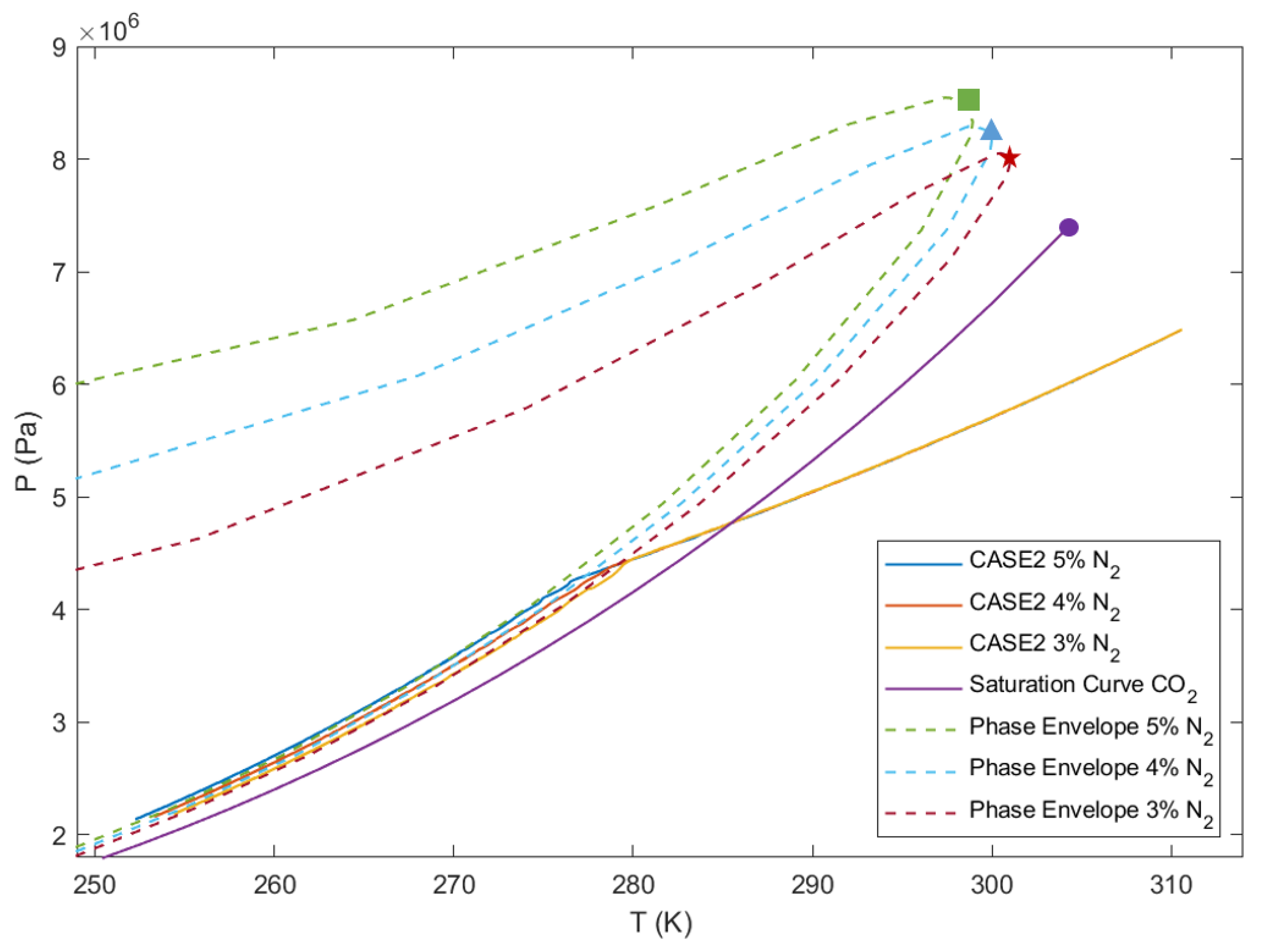
1.3. Introduction to Single- and Multi-Component PT-Diagram

To understand condensation and how it occurs, it is necessary to have a conceptual understanding of thermodynamic diagrams. When the working fluid is a pure single component, the line that separates the gas phase from the liquid phase is known as the coexistence line or saturation curve in the PT-diagram. This is indicated by the purple line in the Figure 1. The gas phase is below the saturation curve and the liquid phase is above it. The extreme point ($P,T$) of this curve is the critical point of the fluid under study, often noted as ($P_c,T_c$). The critical point of pure CO${}_2$ is $P_c$ = 7.377 MPa and $T_c$ = 304.128 K, which is represented by a purple dot in the Figure 1. Above this critical point lies the supercritical fluid zone, where the fluid behaves in a completely different way. Indeed, recent studies have shown that a further classification between liquid-like and gas-like behavior continues in the supercritical zone, as explained in references [15,16].

In the case of a multi-component fluid, the thermodynamic representation and, in particular, the PT diagram of the mixture, are completely different from that of a single-component fluid. Indeed, even with a small amount of impurity added to pure CO${}_2$, the coexistence line separates into two independent lines, the dew line at the vapor side and the bubble line at the liquid side, which constitute the so-called phase envelope. The zone between these lines is the two-phase region. The phase envelope of CO${}_2$ as a main species, with N${}_2$ as impurities of 5%, 4% and 3%, is shown in the dotted lines in Figure 1. The green dotted line shows the phase envelope with 5% N${}_2$, light blue for 4% N${}_2$, and red dotted line for the phase envelope with 3% N${}_2$. In addition, we observe a shift in the critical point ($P_c,T_c$) with the phase envelope, showing that impurities also delay the subcritical/supercritical transition, which occurs at a higher pressure as the amount of impurities increases. The corresponding shift in the critical points is marked with a green square (for 5% N${}_2$), blue triangle (for 4% N${}_2$) and red star (for 3% N${}_2$), while the critical point of pure CO${}_2$ is shown as a purple dot. The solid lines show the numerical results of case 2 (this is a reference to

Table 1. Inlet and outlet conditions of the nozzle from experiments carried out by Lettieri et al. [11].

Case	Inlet Total Pressure ${\mathit{P}}_{\mathit{inlet}}={\mathit{P}}_{\mathit{t}}$ (MPa)	Inlet Total Temperature ${\mathit{T}}_{\mathit{inlet}}={\mathit{T}}_{\mathit{t}}$ (K)	Subsonic Outlet Pressure ${\mathit{P}}_{\mathit{exit}}$ (MPa)
1	5.896	314.67	1.973
2	6.535	311.99	2.281
3	7.353	313.60	2.437
4	7.999	313.94	2.729
5	8.474	313.88	2.805

, which is discussed later in this paper) with N${}_2$ as impurity, where the blue line is 5% N${}_2$, the red line is 4% N${}_2$ and the yellow line is for the 3% N${}_2$ impurity. As the amount of impurity increases, the phase envelope becomes wider as the distance between the dew line and the bubble line increases. In the context of CO${}_2$ with N${}_2$ as an impurity, as the amount of N${}_2$ increases, the deviation of the dew curve from the saturation line of pure CO${}_2$ is not significant, whereas it becomes more significant in relation to the bubble curve. This means that the amount of impurities plays a dominant role in shifting thermodynamic properties on both sides of the phase envelope, but more so on the evaporation side than on the condensation side. Further discussion on the effects of impurities on the (CO${}_2$-impurities) phase envelope can be found in references [7,17].

1.4. Introduction to Two-Phase Flow Modeling

The numerical schemes for simulating two-phase flows, such as the Volume of Fluid method (VOF) [18], Level Set method (LS) [19] and Diffuse Interface method (DIM) [20,21,22], are largely dependent on interface computation. Interface capturing methods explicitly capture the interface in each cell of the computational grid, and interface tracking methods dynamically track the interface by tracking the motion of particles on the interface. The main advantage of working with a DIM-based approach is that satisfying the interface conditions is not explicitly required, as the interface topology is handled automatically, thus making the process computationally efficient. A comprehensive review of DIM can be found in reference [21].

1.5. Introduction to the Real Fluid RFM Model

The simulation of single-phase (liquid or gas) compressible flows has its own set of challenges, mainly due to the possible appearance of shock waves. This, in addition to the presence or appearance of a second phase (cavitation, boiling, etc.), can be quite challenging for the numerical solvers due to the sharp variations of the thermodynamic properties across the subcritical interface as well as across the Widom line, which is generally considered as the transcritical interface, as explained in [15,16]. These numerical challenges of non-linearity of thermodynamic properties due to phase change in subcritical and transcritical regimes make such studies difficult and require employing accurate real fluid equations of state. Indeed, the work of Jafari [16] has demonstrated that the ideal gas equation (EoS) is no longer valid when the conditions are close to the transcritical conditions. Thus, to accurately resolve the sharp gradients of density, pressure and other thermodynamic values, we need a precise real fluid EoS for simultaneously studying two-phase flows with shock formation, evaporation and condensation. Consequently, to be able to simulate such complex phenomena, this work proposes a real fluid model, referred to in this work as RFM.

1.6. Short Overview of VLE Tabulation

In the RFM model, we use a vapor–liquid equilibrium (VLE) tabulation approach to tackle the complexity involved in solving the behavior of multi-component and two-phase simulations. There are several equations of state (EoS) that can be used in VLE calculations to correctly capture thermodynamic properties. SRK-EoS is shown to provide accurate predictions in cryogenic conditions with good prediction of fluid density for lighter species, such as N₂ [15,16,23], where as PR-EoS is said to work better with heavier species such as $n{C}_{12}$H${}_{26}$ [24]. The behaviour of fluids that are close to the supercritical state may require a different EoS from the one that works best under conditions that are far from the supercritical state [14]. Studies show that CPA-EoS works best with polar species such as methanol [25,26]. Recent work by Kheiri et al. [27] provides details on the efficiency of CPA for modeling pure CO${}_2$ and its solubility.

Solving cubic EoS and the iterative treatment of VLE using a flash set of equations is computationally very expensive [28]. Therefore, before starting the numerical simulation, a table is prepared which stores the values of thermodynamic and transport properties for all possible mixtures in a specified range of temperature (T), pressure (P) and mass fraction ($Y_k$, $k=1,N_s-1$), where $N_s$ is the number of species in the mixture. During the simulation run, the various properties are interpolated from the table, giving this approach the name “look-up table approach” in the literature [6,29,30,31]. In this work, an in-house thermodynamic library, IFPEN-Carnot, is used to generate the table, which is 3D in the case of a binary mixture ($N_s=2$). Various real fluid EoS, such as Peng–Robinson (PR), Soave–Redlich–Kwong (SRK) and Cubic-Plus-Association (CPA), are available in this library as thermodynamic closures (details about them are presented later in Section 2.3). In this work, CPA-EoS is used to compute the required properties following the work of Gaballa et al. [26] and Kheiri et al. [27]. This look-up table is generated based on an isothermal–isobaric flash (commonly referred to as TPn-flash) [29,32].

This VLE tabulation method has been implemented in the CONVERGE solver along with the RFM model [33].

1.7. Scope of the Present Study

The present work employs the RFM model, in conjunction with the tabulation approach, in order to reproduce the experimental observations of CO${}_2$ condensation recorded by Lettieri et al. [10]. The primary objective of the work is to show that this equilibrium real fluid approach is capable of accurately capturing the transient appearance of the condensation of the supercritical CO${}_2$ observed experimentally in the divergent part of the de Laval nozzle. The second objective is to demonstrate the significant effects of impurities in CO${}_2$, which has been neglected in previous numerical simulations [8,11,12]. Indeed, as mentioned in the introduction, this can have a considerable impact on the phase diagram of mixtures (CO${}_2$–impurities), which, as we will show in this work, leads, in particular, to different quantities of condensed CO${}_2$. Among the conclusions, this work shows that the results of numerical simulations taking impurities in CO${}_2$ into account are not only closer to real industrial CCS conditions, but also numerically more robust and therefore easier to perform, which was not expected. It is customary to use numerical methods on a simplified model prior to tackling more intricate systems, such as a complete 3D pump. In order to streamline the examination of effects seen in pumps, we performed the study using a 2D De Laval nozzle. This enables us to reduce computational time and complexity while demonstrating the model’s ability to replicate physical phenomena, including phase change.

The key contribution of this article is to propose a real fluid model for accurate and robust two-phase and multicomponent CFD simulations. This study reveals the following features: (1) the structure and dynamics of the de Laval in-nozzle flow including shock waves and condensation, (2) the amount of condensed CO${}_2$ in supersonic nozzle flows and (3) the effects on condensation of the inlet conditions and impurities.

The rest of this article is organized as follows. Section 2 will present the numerical and theoretical methods, including the governing equations and tabulation methods. The description of the experimental data base and the numerical setup are then described in Section 3. Section 4 will present the results discussion, including a comparison of the numerical simulation with the available experimental data. Finally, the conclusion of this study, along with suggestions for future work, is presented in Section 5.

2. Computation Model and Methodology

2.1. The Real Fluid RFM Model

Within the diffuse interface method (DIM), there are many two-phase flow models available, with a number of transport equations ranging from three to seven depending on the initial equilibrium assumptions. This study utilizes a two-phase fully compressible 4-equation model developed at IFPEN, which assumes that the flow system is in full equilibrium (i.e., equilibrium of velocity, pressure, temperature and chemical potential at liquid–vapor interfaces). This model is, therefore, a homogeneous equilibrium model (HEM). It differs from previous HEM models in the thermodynamic closure, which uses a real fluid equation of state for the calculation of the thermodynamic and transport properties, and in the vapor–liquid equilibrium (VLE) procedure, which provides comprehensive knowledge regarding both liquid and gas composition in addition to the local vapor fraction in all cells of the computational grid. Therefore, the RFM model can be seen as a VOF model in which the interface is captured thermodynamically.

2.2. Governing Equations

The following set of governing equations of the CONVERGE CFD solver [33] were used as the basis for the implementation of the proposed real fluid RFM model. This implementation is based on the continuity equation, the species transport equation, the mixture momentum equation and the mixture-specific internal energy equation.

$$\frac{\partial \rho }{\partial t}+\frac{\partial \rho u_i}{\partial x_i}=0$$

(1)

$$\frac{\partial \rho Y_m}{\partial t}+\frac{\partial \rho Y_m{u}_j}{\partial x_j}=\frac{\partial }{\partial x_j}\left(\rho D\frac{\partial Y_m}{\partial x_j}\right),m=\{1\dots N_s-1\}$$

(2)

$$\frac{\partial \rho u_i}{\partial t}+\frac{\partial \rho u_i{u}_j}{\partial x_j}=\frac{\partial P}{\partial x_i}+\frac{\partial {\tau }_{ij}}{\partial x_j}$$

(3)

$$\frac{\partial \rho e}{\partial t}+\frac{\partial \rho e{u}_j}{\partial x_j}=-P\frac{\partial u_j}{\partial x_j}+{\tau }_{ij}\frac{\partial u_i}{\partial x_j}+\frac{\partial }{\partial x_j}(\lambda \frac{\partial T}{\partial x_j})+\frac{\partial }{\partial x_j}(\rho D\sum _m^{}{h}_m\frac{\partial Y_m}{\partial x_j})$$

(4)

where $N_s$ is the number of species, ${\tau }_{ij}$ is the viscous tensor stress and $\rho ,u_i,P,T,e$ are the mixture, density, velocity, pressure, temperature and specific internal energy, respectively.

For the flows dealing with discontinuity due to shock waves, as observed in the de Laval nozzle simulated below, Equation (4) is replaced by the following total energy Equation (5):

$$\frac{\partial \rho E}{\partial t}+\frac{\partial }{\partial x_j}\left(\rho u_{j}E+u_{j}P-u_i{\tau }_{ij}-\lambda \frac{\partial T}{\partial x_j}-\rho D\sum _m^{}{h}_m\frac{\partial Y_m}{\partial x_j}\right)=0$$

(5)

2.3. Thermodynamic Closure and Tabulation Details

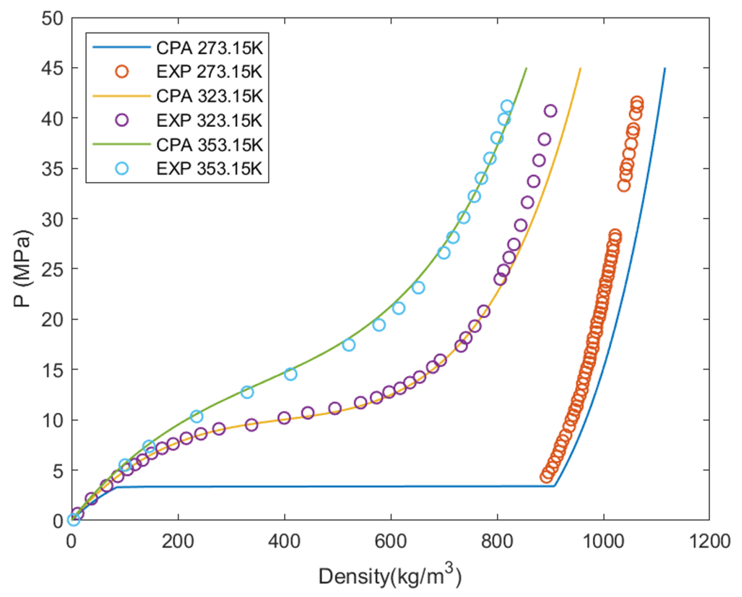
The closure of the above mentioned flow system can be achieved by a real fluid EoS, such as Peng–Robinson (PR) [34], Soave–Redlich–Kwong (SRK) [35,36,37] (they belong to the category of classical cubic EoS [38]) or Cubic-Plus-Association (CPA). Based on the understanding gained from the literature [27,39,40], the present work used CPA as the EoS for the closure. Using this CPA EoS, a uniform look-up table is generated over the entire range of the case’s estimated thermodynamic states. Three inputs to the table are temperature (T), pressure (P) and species mass fraction ($Y_m,m=1,N_s-1$), where $N_s$ is the number of species in the mixture. The IFPEN-Carnot thermodynamic library, based on a robust isothermal–isobaric (TPn)-flash algorithm performs calculations for the vapor–liquid equilibrium (VLE) for each grid point of the look-up table in order to compute the thermodynamic and transport properties in each phase. Then, mixture rules are used to compute these properties for the all specified mixtures in the table. For the input (T,P,Y) parameters, there is a range of maximum values and the number of points to cover this range of input parameters. Thus, the table has a three-dimensional cubic array of values with P, T and $Y_m$ as its axis. Each cell of this array stores more than ten calculated thermodynamic and transport property values. During the run time, for the values that the solver is looking for, a lookup method is performed with a linear interpolation based on the inverse distance weighting method. More details on this can be found in the works of Jafari et al. [41] and Gaballa et al. [26].

2.4. Thermodynamic Validation for CO${}_2$–H${}_{2}S$ Configuration

The ability of the RFM model to simulate the condensation of CO${}_2$ with impurities needs some validation. After an extensive literature search, we found work on CO${}_2$-rich streams with H${}_2$S ($95/5$% by mole%) as an impurity in the experiments of Coquelet et al. [17]. These experiments provide a unique set of experimental data consisting of three isotherms. As shown in Figure 2, the lowest isotherm (273.15 K) crosses the dome in the subcritical region, and the highest isotherm (353.15 K) is in the supercritical region, with the intermediate isotherm (323.15 K) close to the critical point of the mixture (95% CO${}_2$ + 5% H${}_{2}S$). The predictions plotted in the P-$\rho$ diagram (see Figure 2) are obtained with the CPA-EoS, one of the EoS available in the IFPEN-Carnot thermodynamic library. A good agreement between the numerical and experimental is obtained, despite the slight deviation (less than 3%) that occurred at high pressure for the subcritical isotherm (273.15 K) in the liquid side.

Although the validation is not on the mixture of interest (CO${}_2$ + N${}_2$), for subsequent de Laval nozzle simulations, H${}_2$S is one of the impurities in CO${}_2$-rich vapors and having validation of one of the impurities in industrial CO${}_2$ should give more confidence in the following simulations where condensation takes place and in one of the main expected numerical results.

3. Experimental and Computational Methods

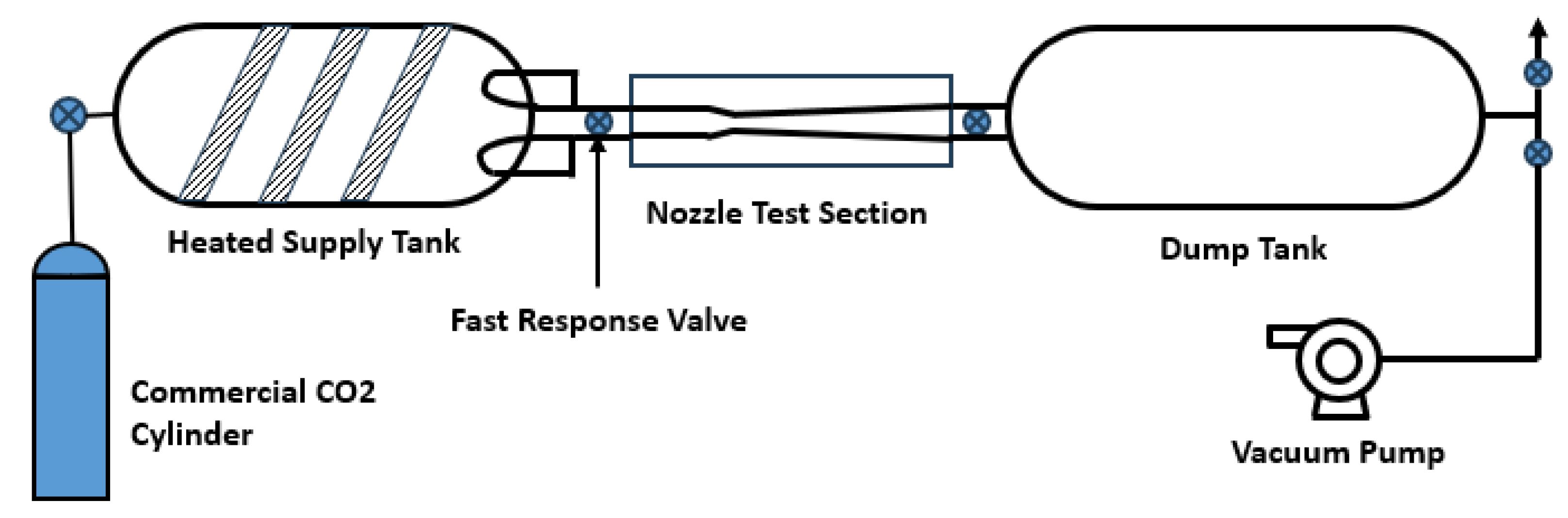
3.1. De Laval Nozzle Experiments

In the experiments carried out by Lettieri et al. [10,11], the condensation was recorded in the converging–diverging nozzle (also known as a de Laval Nozzle). The setup of the experiments is shown in Figure 3 and the experimental conditions in terms of total pressure ($P_t$) and temperature ($T_t$) are provided in Table 1. The experiments were carried out over a wide range of pressures. The liquid CO${}_2$ flows from the high pressure tank on the left. The transparent observation section of the de Laval nozzle is in the center of the experiment (between the two valves) to which the gaseous CO${}_2$ is passed. This gas is then collected in the dump tank connected to the outlet at the exit of the nozzle, which is then connected to the vacuum pump to evacuate the collected gas. To control the flow, high-response time valves are connected near the inlet and outlet of the test nozzle section.

The experiments start with a subcritical inlet pressure furthest from the critical point of pure CO${}_2$ (case 1 and case 2), and progressively carry out four further series of experiments where the inlet pressure of case 3 is closest to the critical pressure point of pure CO${}_2$, then cases 4 and 5 are taken into supercritical pressure states still relative to the critical point of pure CO${}_2$ ($P_c$ = 7.377 MPa and $T_c$ = 304.128 K). The resulting database mainly comprises the following:

• The steady state pressure profiles along the nozzle;
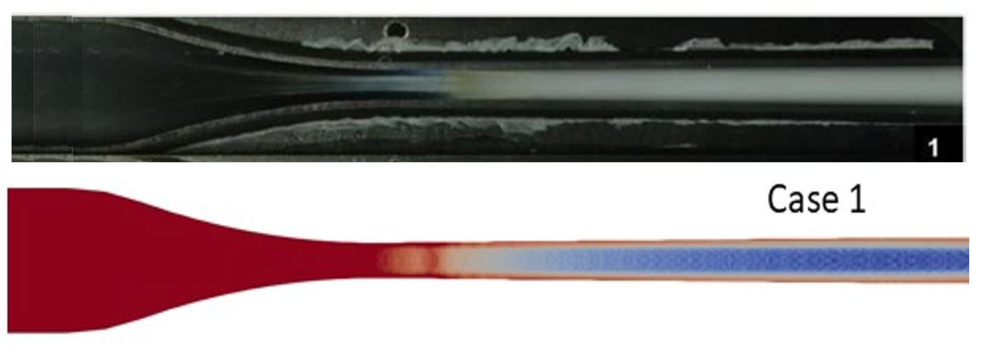
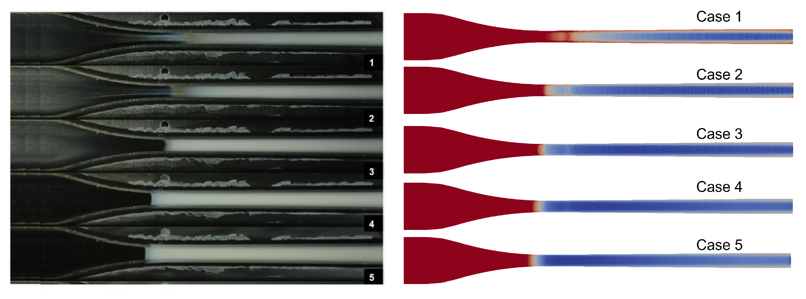
• The shadography images of the the nozzle showing the two-phase (condensation) region.

The work in references [10,11] mentions CO${}_2$ as the fluid used, however, the paper does not address the exact amount of impurities present initially in the CO${}_2$ gas used in the experiments. Our hypothesis is that, even if the CO${}_2$ used is of high quality, it still has traces of impurities that play a role, even if they enter the test section through the presence of air before the test section is filled with the working fluid. This current work focuses on the effect of impurities on the condensation observed in the de Laval nozzle. Thus, for the scope of this paper, we limit our study with the operating details shown in Table 1.

3.2. Computational Setup

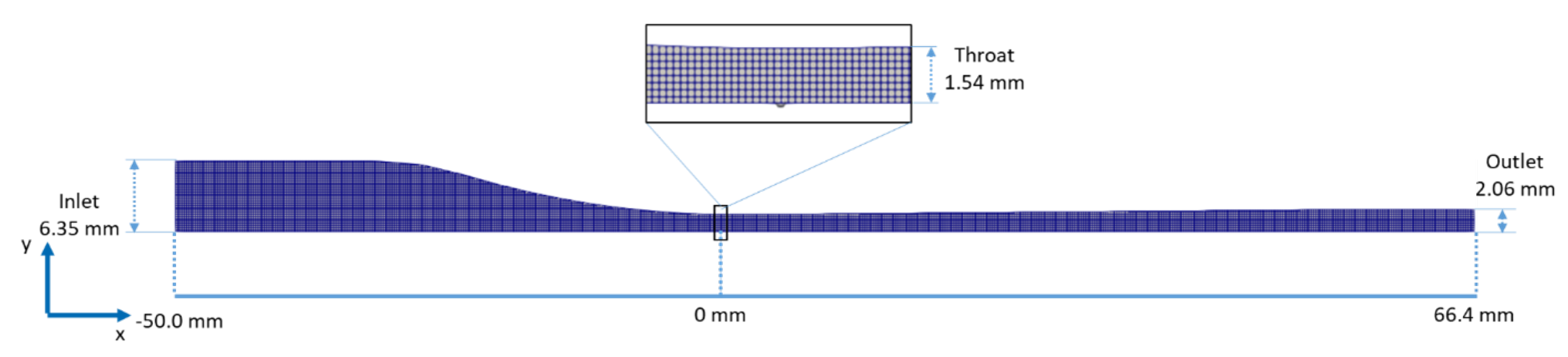
3.2.1. Computational Grid

A two-dimensional (2D) computational domain is used in the current work. The computational model is created in CONVERGE Studio and the appropriate boundary conditions are applied. The nozzle data are taken from references [11,12]. The inlet, throat and outlet radii are 6.35 mm, 1.54 mm and 2.06 mm, respectively. The length of the nozzle is 116.4 mm with the coordinate system zeroed at the throat of the nozzle, as depicted in Figure 4.

The structured grid mesh is generated with 0.2 mm base grid spacing in the stream-wise and span-wise directions. The mesh structure is shown in Figure 4. The mesh has been successively refined by up to eight cells in the half-throat to obtain grid-independent results, as recommended by Lettieri [10,11].

3.2.2. Boundary Conditions

The lower boundary is set as a symmetry boundary condition (BC). The upper boundary is defined as an isothermal wall with a specified temperature taken equal to ($T_t$), as given in Table 1. More precisely, a standard wall function is used with no-slip boundary condition. Because the simulations carried out in this work are intended to solve the transient period, including the acceleration of the flow in the convergent up to the critical flow rate, then, for the shock wave initiation and movement towards the nozzle outlet at the right side of the grid, a transonic pressure outlet BC is used with a transition from subsonic to supersonic with a Mach number in the range (0.9–1.1). A Neumann BC is used when the Mach number is greater than 1.1, while a pressure is specified at the outlet when the Mach number is smaller than 0.9. This outlet pressure is obtained by linearly relaxing the pressure from its initial value to a relatively low pressure ($P_{exit}$), in order to gradually accelerate the flow through the nozzle to its steady state. The analytical calculations performed give us the values of the pressure $P_{exit}$, as listed in the last column of Table 1. The relaxation time is estimated at a tenth of a second.At the inlet, we use the total pressure and temperature, given in Table 1, as BC. In addition, the inlet mass fraction of nitrogen N${}_2$ is specified, in addition to the CO${}_2$, in order to investigate the effects of the impurities on the CO${}_2$ flow.

3.2.3. Initial Conditions

At the start of the simulations (t = 0), we impose $P_{inlet}$ and $T_{inlet}$ as initial conditions throughout the domain (at each grid point) with the flow specified at rest. As we are dealing with CO${}_2$ with N${}_2$ as impurity, we initialize the mass fraction of these species as initial conditions, in a way consistent with the input BC. It is worth noting that this composition does not vary throughout the simulation because we are running non-reactive simulations. The simulations were run simultaneously to perform a complete study of the effect of the impurity fraction on condensation. Based on understanding from the literature, we first carried out a study with three simulations with three mass fractions of N${}_2$ as the impurity (3%, 4%, 5%). After analysing these initial simulations, based on the computational efforts and cost, the second part of the simulations, including the five experimental cases presented in Table 1, was carried out with a fixed species composition of 95% CO${}_2$ with 5% N${}_2$ as the impurity.

3.2.4. Numerical Schemes, Models and Thermodynamic Table

RANS transient simulations with the proposed RFM model are performed using the $k\omega$-$SST$ turbulence model [42]. The numerical solution of the transport equations is based on a pressure-based solver with a modified Pressure Implicit with Splitting Operator (PISO) algorithm for real fluid simulations. Such a modified PISO has been validated in previous work, such as in references [16,24,26]. The spatial discretization is second-order accurate with a central difference scheme and the time integration is performed using a Crank–Nicolson scheme for the momentum equation and an implicit first-order Euler scheme for the rest of the equations. The time step is not fixed in the simulations as the CONVERGE solver [33] does a good job in adjusting the step, as per the requirements based on the Courant–Friedrichs–Lewy (CFL) number. The initial time step of the simulations is set to one microsecond.

A 3D table covering the full range of (P-T-Y) values for the binary mixture (CO${}_2$ + N${}_2$) was generated for all the simulation conditions. This thermodynamic table has its three axes (1401 × 201 × 6) as range of pressure (1.5–8.5 MPa), temperature (240–340 K) and species mass fraction Y_{CO${}_2$} (0.95–1). The employed thermodynamic table resolution is based on previous studies [16,24,25,26,43], and will be shown to provide sufficiently accurate results in the following sections. In addition, table sensitivity was independently performed and the above mentioned table matrix size was found to be the most suitable.

4. Results and Discussions

Contrary to previous de Laval nozzle simulations with CO${}_2$ performed with steady state solvers (see references [11,12], for instance), the present work employs an unsteady numerical method to analyse (1) the acceleration of the flow, (2) the transition from subsonic to supersonic near the nozzle throat and in the divergent part and (3) the interaction between the shock wave and CO${}_2$ condensation.

4.1. Transient Flow Characteristics

The flow develops transiently in the de Laval nozzle as the outlet pressure relaxes to the estimated ($P_{exit}$) value given in Table 1. The flow acceleration from subsonic to fully supersonic regimes in the nozzle diverging part is explained here based on the numerical results of Case 1 with the four following steps:

• A subsonic regime in both the converging and diverging part of the de Laval nozzle. In this first step, the flow accelerates progressively in the converging part, but it decelerates along the diverging part. The Mach number is still lower than one in the entire nozzle, and has its maximum value at the throat, as shown Figure 5b. In addition, the pressure profile is also shown in Figure 5a to progressively decrease in the converging part, but it increases along the diverging part towards ($P_{exit}$). Figure 5c and Figure 6a show that the condensation is not present in the nozzle in this subsonic regime and, consequently, the nozzle is only filled in the gas phase.
• A sonic regime where the flow has been accelerated up to a Mach number of one (see Figure 5e) happens simultaneously with the throat pressure decreasing to a critical value (approximately 3.3 MPa), as shown in Figure 5d. Figure 5f and Figure 6b show that the presence of condensation is still not observed just at the moment of meeting critical conditions.
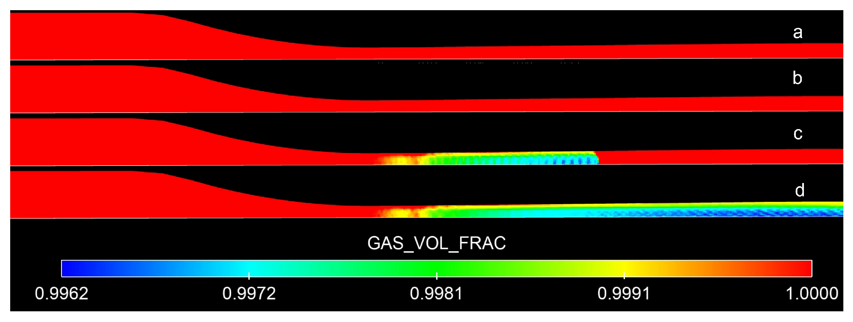
• A supersonic/subsonic transition regime. In fact, because the pressure at the nozzle outlet ($P_{exit}$ = 1.973 MPa) is still lower than the pressure value at the throat (3.3 MPa), the flow continues to accelerate and reaches the supersonic regime in the diverging section, as shown in Figure 5h,g. In these figures, a shock wave created just after the throat, and moving towards the nozzle outlet inside the divergent part, is successfully captured when the outlet pressure is relaxed towards ($P_{exit}$). The presence of condensation is observed in Figure 6c, as well as the profiles of gas volume fraction in Figure 5i.
• A fully supersonic regime in the diverging part of the de Laval nozzle is finally obtained when the shock wave leaves the computational domain, as shown in Figure 5j,k. However, the converging part remains in the subsonic regime. The nozzle is filled with condensation from the throat to the exit downstream. Such fully supersonic acceleration of the flow through a converging–diverging nozzle is used in practical applications such as rocket engine lift-off.

4.2. CO${}_2$ Condensation and Shock Wave Interaction

In Figure 5h,i,k,l, and Figure 6c,d one can observe the appearance of condensation at the same time as the formation of the throat shock. The condensation progresses along the entire diverging section of the diverging part with the shock wave. Indeed, condensation appears due to the correlation of the drop in pressure and temperature slightly below the “dew line”. The dew line is the right branch of the phase envelope that marks the transition boundary from vapor to liquid (i.e., appearance or disappearance of condensation), as depicted in Figure 1.

After the shock has left the nozzle, the diverging section is completely filled with a cloud of liquid. The visual confirmation of the condensation is also shown in Figure 7, where the upper part of the image is taken from the experiments of Lettieri et al. [11] and the lower part is from the numerical simulation of case 1 when the fully supersonic regime is reached. This figure is from the simulation with 95% CO${}_2$ and 5% N${}_2$. Two main observations in this figure are that (1) the starting point of the condensation is at the throat, which is very well reproduced in the simulations, and (2) the condensation front at the throat is somewhat diffused in a very similar way as it appears in the experimental image. Condensation is present throughout the second half of the nozzle. However, a layer with lower condensation can be seen near the walls in Figure 7, in both the numerical and experimental images. This wall boundary layer seems to be due to the higher specified wall temperature, at least in the simulations.

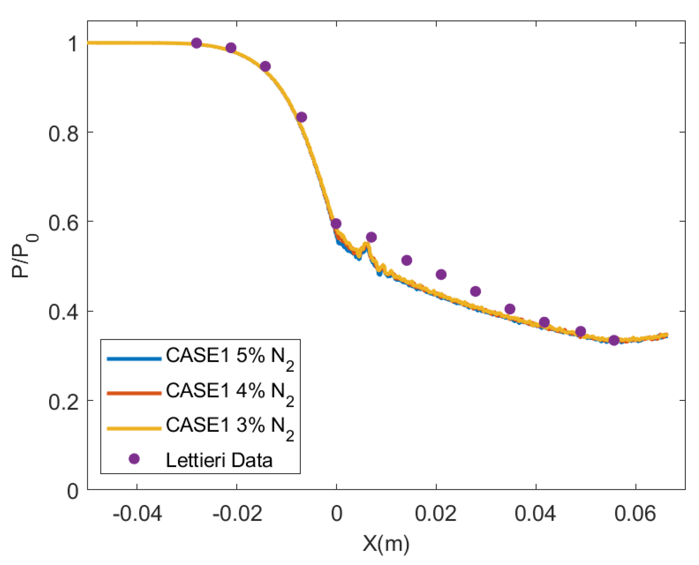
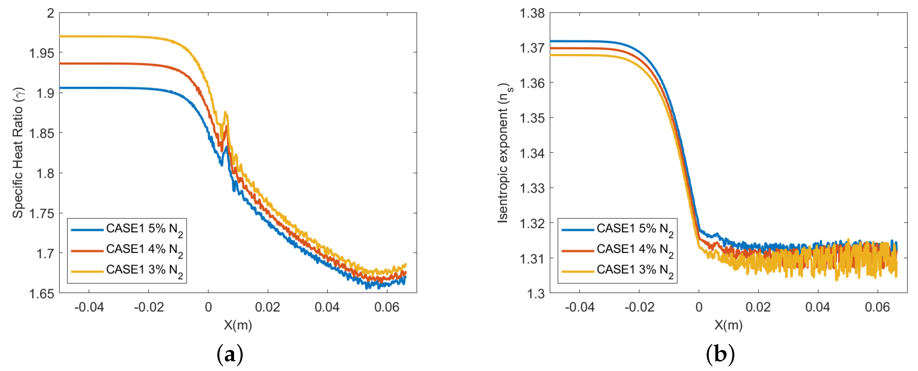
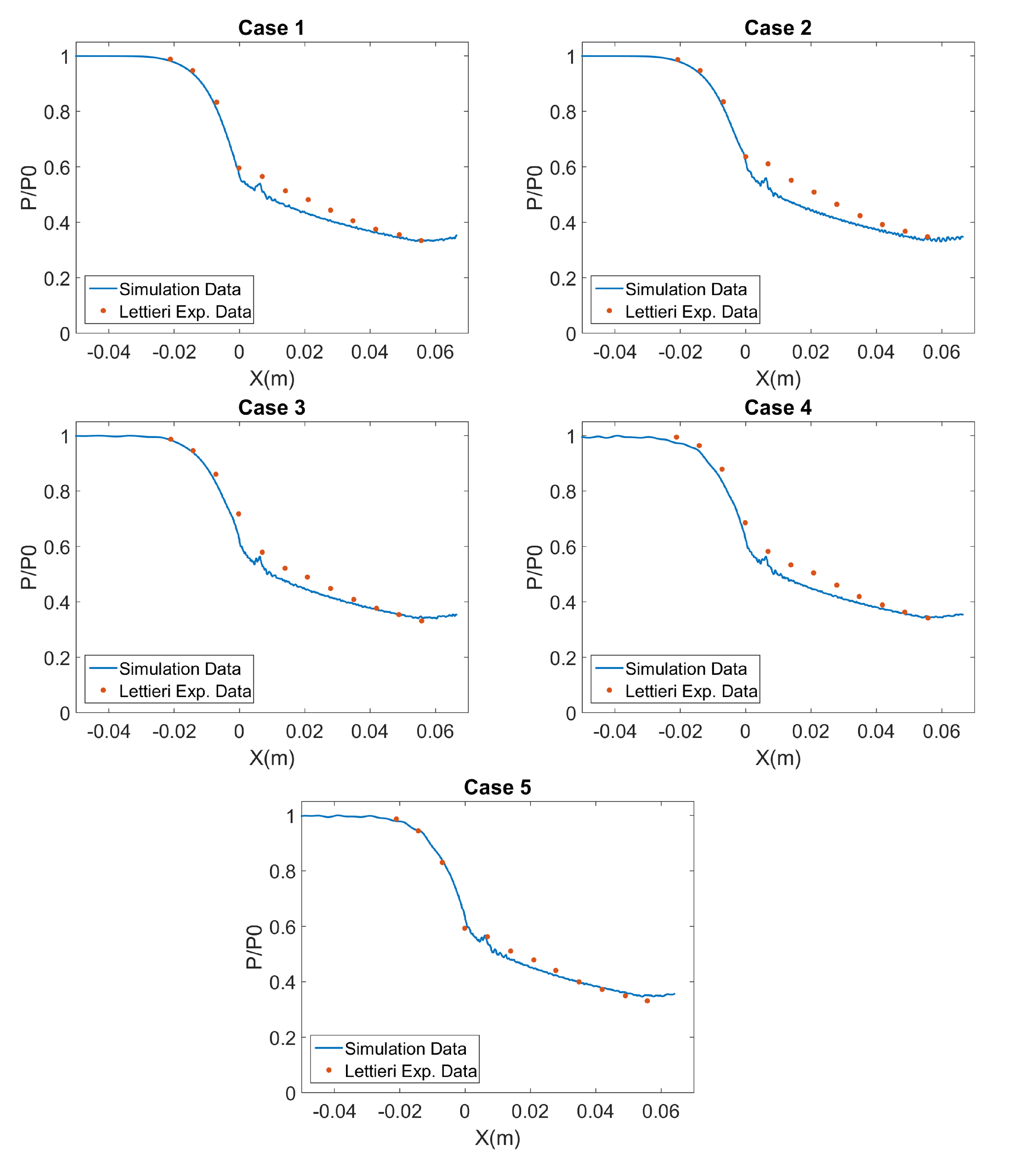
4.3. Nozzle Axial Profiles Results

To examine the pressure readings from the experiments and simulations, we have plotted the pressure profiles in Figure 8. The pressure recordings along the nozzle axis are normalized with the inlet total pressure for each simulation. These pressure profile is typical of the behaviour observed where the flow is fully supersonic in the divergent part of the nozzle. We observe that the pressure profile overlaps, irrespective of the amount of impurity in the gas mixture. The pressure profile of the simulations matches one of the experiments perfectly in the converging region of the nozzle. However, a slight difference can be observed after the throat, where a pressure oscillation occurs in this almost sonic part of the nozzle. The variation in CO${}_2$ properties due to local flow acceleration and phase change can also be considered as a possible mechanism to explain this oscillation problem observed near the nozzle’s critical point, as discussed in reference [9]. Still, this oscillation issue in the pressure profiles has not been captured experimentally. Overall, the match with the experimental data is satisfactory.

The temperature and Mach number behavior are shown in Figure 9. We can see that impurities do not affect these profiles very much, although a slight temperature rise can be noted in the divergent part of the nozzle when the amount of impurity is reduced. Indeed, changing the amount of N${}_2$ in the mixture obviously leads to thermodynamic and transport property variations. For example, a specific heat ratio ($\gamma$) oscillation can be seen in Figure 10a at the same place (close to the condensation cloud interface) as the pressure oscillation. Similar interface fluctuations of the specific heat capacity due to real fluid non-linearity have been discussed in Jafari et al. [16,41]. The importance of considering the real fluid effect on the thermodynamic and transport properties has been also highlighted by Baltadjiev et al. [9]. They demonstrated that the various theoretical relationships often employed for convergent–divergent nozzle calculations, and expressed in terms of the isentropic exponent $\gamma$ in an ideal gas formulation, must be modified in terms of a modified exponent $n_s=\frac{\gamma }{{\beta }_{T}P}$ when a real fluid formulation is adopted, where ${\beta }_T$ is the isothermal compressibility. Figure 10b reveals that $n_s$ is less sensitive to the presence of impurities and, indeed, it is appropriate for basic calculations of compressible flow relationships for a real fluid in converging–diverging nozzles. This shows the importance of having a real fluid model over the ideal gas assumptions in this type of study.

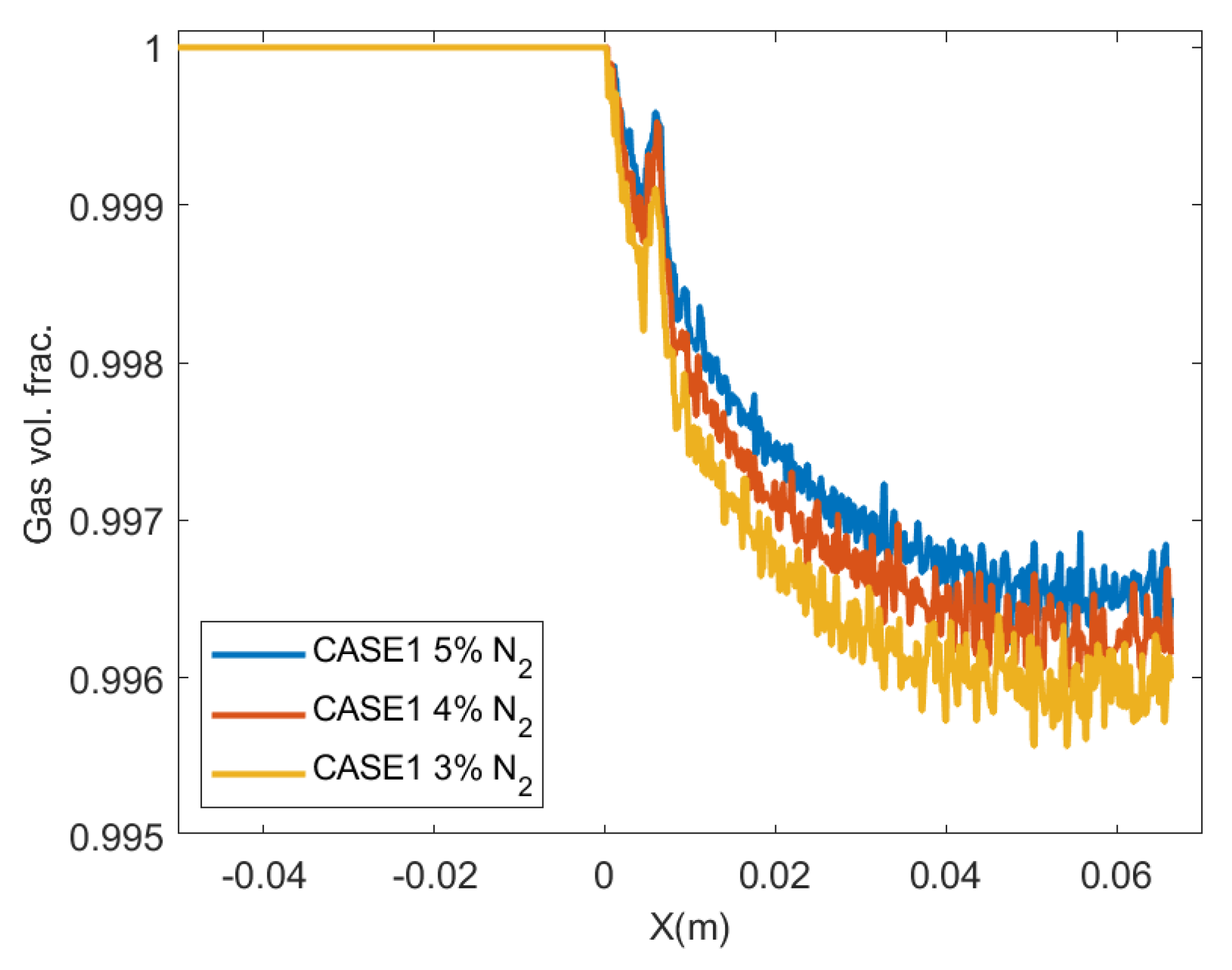
4.4. Effect of Impurities on the Amount of Condensation

The proportion of condensation recorded for case 1 is plotted along the nozzle on the X axis in Figure 11 through the decrease in gas volume fraction (${\alpha }_{gas}$). As can be seen from the numerical results in Figure 7, there is no condensation observed in the converging section of the nozzle. This is seen as a straight line in Figure 11 from the nozzle inlet to the throat, at X = 0. The presence of condensation is seen quantitatively after the throat in the diverging section of the nozzle. The highest ${\alpha }_{liq}$ value for case 1 is of the order of 0.004, corresponding to the 3% impurity case, as shown in Figure 11. In fact, the greater the quantity of impurities present in the initial CO${}_2$, the lower the condensation. This implies that, in the case of pure CO${}_2$, a very high amount of condensation should have been obtained, as illustrated in Figure 12, for case 1 conditions at the fully supersonic regime. In this figure, only a few cells are filled with liquid in the divergent part of the nozzle. This may be due to the increased tensile strength of the fluid as the quantity of impurities decreases.

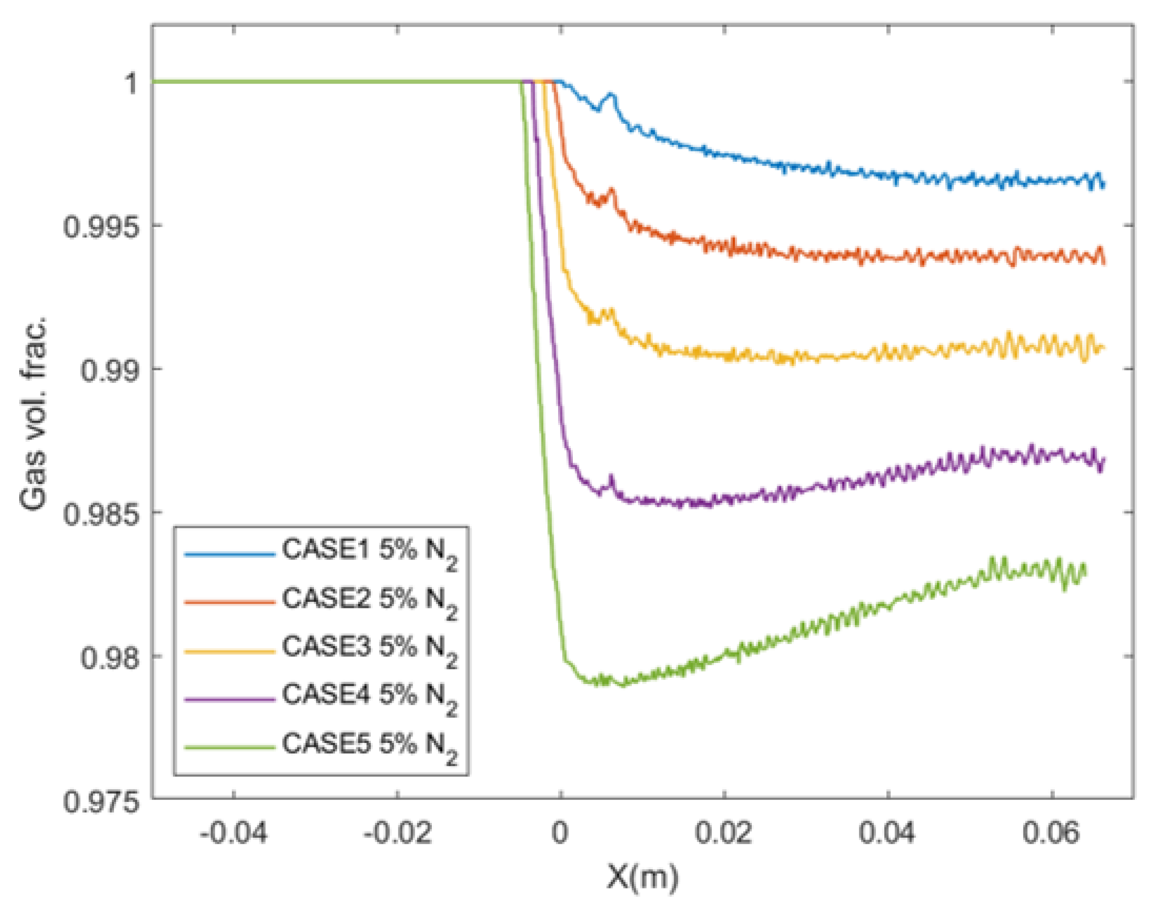
4.5. Effect of Operating Pressure on the Amount of Condensation

Figure 13 shows the effect of the inlet total pressure (given in Table 1) on the condensation observed over the center-line axial profile. The plot shows the amounts of condensation, as in Figure 11. From case 1 (the furthest from the CO${}_2$ critical point) to Case 5 (the closest to the CO${}_2$ critical point), an acceleration of condensation is observed, as the initial slope of the gas volume fraction increases near the throat. Furthermore, the condensation front moves before the nozzle throat (position at X = 0) and a sharper two-phase gradient is also observed as the inlet pressure is increased from Case 1 to Case 5. These numerical results are qualitatively corroborated by the experimental and numerical images shown in Figure 14. It is also worth noting in Figure 13 that, in Case 4 and especially Case 5, some of the liquid condensed near the throat evaporated before reaching the nozzle outlet section. This demonstrates the ability of the RFM model used in this work to simulate both condensation and evaporation.

Finally, Figure 15 gathers all the calculated pressure axial profiles along the nozzle and compares them with the measured pressure profiles obtained from the Lettieri experiments [10,11]. The instantaneous local center-line pressure obtained at the fully supersonic regime are plotted. It is normalized by the inlet total pressure. The RFM model results are in fairly good agreement with the data. The onset of condensation for the highest pressure case 5 occurs well before the throat (upstream of the nozzle throat) and represents the challenge to the CFD calculations due to its proximity to the critical point and the rapid and sharp condensation front. Lettieri et al. [10,11] also comment on the experimental results for this condition, noting that additional high pressure experiments need to be performed to resolve the issue. From a CFD point of view, this work provides the validation in terms of capturing the main characteristics as observed in the experiments.

5. Conclusions

In this article, the effect of impurities on the condensation of CO${}_2$ is studied using the tabulated RFM model implemented in the CONVERGE solver. The simulations are carried out at five operating conditions, starting at 58 bar (lower than the CO${}_2$ critical point) up to 84 bar (higher than the critical point of CO${}_2$). The transient simulations show that, when the nozzle outlet pressure is reduced, the flow is accelerated and the different known nozzle regimes (subsonic, sonic and supersonic) take place. As the flow is accelerated by the progression of the shock, the temperature is reduced and this is also accompanied by the progression of condensation in the diverging part of the nozzle. This study reveals the following features:

• The structure and dynamics of the de Laval in-nozzle flow include shock waves, condensation and the amount of condensed CO${}_2$ in supersonic nozzle flows.
• This amount increases as the inlet operating condition is moved close to the supercritical state.
• The effects on condensation of the inlet conditions and impurities.
• The amount of condensation increases as the amount of impurities decreases. Consequently, the present numerical study has shown that the condensation of CO${}_2$ observed experimentally in the de Laval nozzle can hardly be produced without adding a small amount of impurity.

Finally, it is recommended that the various impurities present in industrial CO${}_2$ be taken into account when simulating CO${}_2$ flows from pipelines and pumps used for carbon capture, utilization and storage (CCUS).

References

1. The Intergovernmental Panel on Climate Change (IPCC) Is the United Nations Body for Assessing the Science Related to Climate Change. Available online: https://www.ipcc.ch/ (accessed on 4 July 2023).
2. Zhao, X.; Ji, G.; Liu, W.; He, X.; Anthony, E.J.; Zhao, M. Mesoporous MgO promoted with NaNO3/NaNO2 for rapid and high-capacity CO2 capture at moderate temperatures. Chem. Eng. J. 2018, 332, 216–226. [Google Scholar] [CrossRef]
3. Chapoy, A.; Nazeri, M.; Kapateh, M.; Burgass, R.; Coquelet, C.; Tohidi, B. Effect of impurities on thermophysical properties and phase behaviour of a CO2-rich system in CCS. Int. J. Greenh. Gas Control. 2013, 19, 92–100. [Google Scholar] [CrossRef]
4. Sterpenich, J.; Dubessy, J.; Pironon, J.; Renard, S.; Caumon, M.C.; Randi, A.; Jaubert, J.N.; Favre, E.; Roizard, D.; Parmentier, M.; et al. Role of Impurities on CO2 Injection: Experimental and Numerical Simulations of Thermodynamic Properties of Water-salt-gas Mixtures (CO2 + Co-injected Gases) Under Geological Storage Conditions. Energy Procedia 2013, 37, 3638–3645. [Google Scholar] [CrossRef]
5. de Visser, E.; Hendriks, C.; Barrio, M.; Mølnvik, M.J.; de Koeijer, G.; Liljemark, S.; Le Gallo, Y. Dynamis CO2 quality recommendations. Int. J. Greenh. Gas Control. 2008, 2, 478–484. [Google Scholar] [CrossRef]
6. Brown, S.; Peristeras, L.D.; Martynov, S.; Porter, R.T.J.; Mahgerefteh, H.; Nikolaidis, I.K.; Boulougouris, G.C.; Tsangaris, D.M.; Economou, I.G. Thermodynamic interpolation for the simulation of two-phase flow of non-ideal mixtures. Comput. Chem. Eng. 2016, 95, 49–57. [Google Scholar] [CrossRef]
7. Zhao, Q.; Li, Y.X. The influence of impurities on the transportation safety of an anthropogenic CO2 pipeline. Process. Saf. Environ. Prot. 2014, 92, 80–92. [Google Scholar] [CrossRef]
8. Brinckman, K.W.; Hosangadi, A.; Liu, Z.; Weathers, T. Numerical Simulation of Non-Equilibrium Condensation in Supercritical CO2 Compressors. In Turbo Expo Power for Land, Sea and Air, Proceedings of the ASME Turbo Expo 2018: Turbomachinery Technical Conference and Exposition, Oslo, Norway, 11–15 June 2018; Volume 9: Oil and Gas Applications; Supercritical CO2 Power Cycles; Wind Energy; American Society of Mechanical Engineers: New York, NY, USA, 2018; p. 06172019. [Google Scholar] [CrossRef]
9. Baltadjiev, N.D.; Lettieri, C.; Spakovszky, Z.S. An Investigation of Real Gas Effects in Supercritical CO2 Centrifugal Compressors. J. Turbomach. 2015, 137, 091003. [Google Scholar] [CrossRef]
10. Lettieri, C.; Yang, D.; Spakovszky, Z. An Investigation of Condensation Effects in Supercritical Carbon Dioxide Compressors. J. Eng. Gas Turbines Power 2015, 137, 082602. [Google Scholar] [CrossRef]
11. Lettieri, C.; Paxson, D.; Spakovszky, Z.; Bryanston-Cross, P. Characterization of Nonequilibrium Condensation of Supercritical Carbon Dioxide in a de Laval Nozzle. J. Eng. Gas Turbines Power 2018, 140, 041701. [Google Scholar] [CrossRef]
12. Romei, A.; Persico, G. Computational fluid-dynamic modelling of two-phase compressible flows of carbon dioxide in supercritical conditions. Appl. Therm. Eng. 2021, 190, 116816. [Google Scholar] [CrossRef]
13. Nakagawa, M.; Berana, M.S.; Kishine, A. Supersonic two-phase flow of CO2 through converging–diverging nozzles for the ejector refrigeration cycle. Int. J. Refrig. 2009, 32, 1195–1202. [Google Scholar] [CrossRef]
14. Zhao, H.; Quan, S.; Dai, M.; Pomraning, E.; Senecal, P.K.; Xue, Q.; Battistoni, M.; Som, S. Validation of a Three-Dimensional Internal Nozzle Flow Model Including Automatic Mesh Generation and Cavitation Effects. J. Eng. Gas Turbines Power 2014, 136, 092603. [Google Scholar] [CrossRef]
15. Banuti, D.T. Crossing the Widom-line—Supercritical pseudo-boiling. J. Supercrit. Fluids 2015, 98, 12–16. [Google Scholar] [CrossRef]
16. Jafari, S.; Gaballa, H.; Habchi, C.; de Hemptinne, J.C. Towards Understanding the Structure of Subcritical and Transcritical Liquid–Gas Interfaces Using a Tabulated Real Fluid Modeling Approach. Energies 2021, 14, 5621. [Google Scholar] [CrossRef]
17. Coquelet, C.; Stringari, P.; Hajiw, M.; Gonzalez, A.; Pereira, L.; Nazeri, M.; Burgass, R.; Chapoy, A. Transport of CO2: Presentation of New Thermophysical Property Measurements and Phase Diagrams. Energy Procedia 2017, 114, 6844–6859. [Google Scholar] [CrossRef]
18. Hirt, C.; Nichols, B. Volume of fluid (VOF) method for the dynamics of free boundaries. J. Comput. Phys. 1981, 39, 201–225. [Google Scholar] [CrossRef]
19. Osher, S.; Fedkiw, R.P. Level Set Methods: An Overview and Some Recent Results. J. Comput. Phys. 2001, 169, 463–502. [Google Scholar] [CrossRef]
20. Baer, M.R.; Nunziato, J.W. A two-phase mixture theory for the deflagration-to-detonation transition (ddt) in reactive granular materials. Int. J. Multiph. Flow 1986, 12, 861–889. [Google Scholar] [CrossRef]
21. Saurel, R.; Pantano, C. Diffuse-Interface Capturing Methods for Compressible Two-Phase Flows. Annu. Rev. Fluid Mech. 2018, 50, 105–130. [Google Scholar] [CrossRef]
22. Cahn, J.W.; Hilliard, J.E. Free Energy of a Nonuniform System. I. Interfacial Free Energy. J. Chem. Phys. 1958, 28, 258–267. [Google Scholar] [CrossRef]
23. Linstrom, P. NIST Chemistry WebBook, NIST Standard Reference Database 69; NIST: Gaithersburg, MD, USA, 2023. [Google Scholar] [CrossRef]
24. Gaballa, H.; Habchi, C.; de Hemptinne, J.C. Modeling and LES of high-pressure liquid injection under evaporating and non-evaporating conditions by a real fluid model and surface density approach. Int. J. Multiph. Flow 2023, 160, 104372. [Google Scholar] [CrossRef]
25. Gaballa, H.; Jafari, S.; Di-Lella, A.; Habchi, C.; de Hemptinne, J.C. A tabulated real-fluid modeling approach applied to renewable dual-fuel evaporation and mixing. In Proceedings of the International Conference on Liquid Atomization and Spray Systems (ICLASS), Edinburgh, UK, 30 August–2 September 2021; Volume 1. [Google Scholar] [CrossRef]
26. Gaballa, H.; Jafari, S.; Habchi, C.; de Hemptinne, J.C. Numerical investigation of droplet evaporation in high-pressure dual-fuel conditions using a tabulated real-fluid model. Int. J. Heat Mass Transf. 2022, 189, 122671. [Google Scholar] [CrossRef]
27. Kheiri, A.; Afsharpour, A. The CPA EoS application to model CO2 and H2S simultaneous solubility in ionic liquid [C2mim][PF6]. Pet. Sci. Technol. 2018, 36, 944–950. [Google Scholar] [CrossRef]
28. Yang, S.; Habchi, C. Real-fluid phase transition in cavitation modeling considering dissolved non-condensable gas. Phys. Fluids 2020, 32, 032102. [Google Scholar] [CrossRef]
29. Yi, P.; Yang, S.; Habchi, C.; Lugo, R. A multicomponent real-fluid fully compressible four-equation model for two-phase flow with phase change. Phys. Fluids 2019, 31, 026102. [Google Scholar] [CrossRef]
30. de Lorenzo, M.; Lafon, P.; Di Matteo, M.; Pelanti, M.; Seynhaeve, J.M.; Bartosiewicz, Y. Homogeneous two-phase flow models and accurate steam-water table look-up method for fast transient simulations. Int. J. Multiph. Flow 2017, 95, 199–219. [Google Scholar] [CrossRef]
31. Föll, F.; Hitz, T.; Müller, C.; Munz, C.D.; Dumbser, M. On the use of tabulated equations of state for multi-phase simulations in the homogeneous equilibrium limit. Shock Waves 2019, 29, 769–793. [Google Scholar] [CrossRef]
32. Yang, S.; Yi, P.; Habchi, C. Real-fluid injection modeling and LES simulation of the ECN Spray A injector using a fully compressible two-phase flow approach. Int. J. Multiph. Flow 2020, 122, 103145. [Google Scholar] [CrossRef]
33. Richards, K.J.; Senecal, P.K.; Pomraning, E. CONVERGE 3.1; Convergent Science: Madison, WI, USA, 2023. [Google Scholar]
34. Peng, D.Y.; Robinson, D.B. A New Two-Constant Equation of State. Ind. Eng. Chem. Fundam. 1976, 15, 59–64. [Google Scholar] [CrossRef]
35. Soave, G. Equilibrium constants from a modified Redlich-Kwong equation of state. Chem. Eng. Sci. 1972, 27, 1197–1203. [Google Scholar] [CrossRef]
36. Péneloux, A.; Rauzy, E.; Fréze, R. A consistent correction for Redlich-Kwong-Soave volumes. Fluid Phase Equilibria 1982, 8, 7–23. [Google Scholar] [CrossRef]
37. Redlich, O.; Kwong, J.N.S. On the thermodynamics of solutions; an equation of state; fugacities of gaseous solutions. Chem. Rev. 1949, 44, 233–244. [Google Scholar] [CrossRef] [PubMed]
38. Kontogeorgis, G.M.; Michelsen, M.L.; Folas, G.K.; Derawi, S.; von Solms, N.; Stenby, E.H. Ten Years with the CPA (Cubic-Plus-Association) Equation of State. Part 1. Pure Compounds and Self-Associating Systems. Ind. Eng. Chem. Res. 2006, 45, 4855–4868. [Google Scholar] [CrossRef]
39. Oliveira, M.; Coutinho, J.; Queimada, A. Mutual solubilities of hydrocarbons and water with the CPA EoS. Fluid Phase Equilibria 2007, 258, 58–66. [Google Scholar] [CrossRef]
40. Palma, A.M.; Oliveira, M.B.; Queimada, A.J.; Coutinho, J.A. Re-evaluating the CPA EoS for improving critical points and derivative properties description. Fluid Phase Equilibria 2017, 436, 85–97. [Google Scholar] [CrossRef]
41. Jafari, S.; Gaballa, H.; Habchi, C.; de Hemptinne, J.C.; Mougin, P. Exploring the interaction between phase separation and turbulent fluid dynamics in multi-species supercritical jets using a tabulated real-fluid model. J. Supercrit. Fluids 2022, 184, 105557. [Google Scholar] [CrossRef]
42. Menter, F.R. Two-equation eddy-viscosity turbulence models for engineering applications. AIAA J. 1994, 32, 1598–1605. [Google Scholar] [CrossRef]
43. Gaballa, H.; Jafari, S.; Di-Lella, A.; Habchi, C.; de Hemptinne, J.C. A tabulated real-fluid modeling approach applied to cryogenic LN2-H2 jets evaporation and mixing at transcritical regime. In Proceedings of the International Conference on Liquid Atomization and Spray Systems (ICLASS), Edinburgh, UK, 30 August–2 September 2021; Volume 1. [Google Scholar] [CrossRef]
Figure 1. Pressure -Temperature diagrams of three cases with various % N 2 as impurity. This figure also shows the (P,T)-path during the gas expansion (represented by the yellow curve) of 95% CO2. This curve crossing over on the dew line (on green dashed phase envelope) represents the appearance of condensation in the nozzle. Similar behaviour is seen for 96% and 97% CO 2 . The saturation line of pure CO 2 is also represented for the comparison with the phase envelope location in the (P,T)-plane. Critical points are represented by different symbols depending on the quantity of impurities.
Applsci 13 10863 g001
Figure 2. Isotherms in the P- ρ diagram for the CO 2 –H 2 S mixture. Predictions obtained with CPA-EoS are compared to the Coquelet et al. [17] experimental data sets. Experimental results are shown as ‘o’ marker and modeling results as solid lines (colors online). The isotherms follow the trends observed in the experimental data set and have agreement at high pressures and densities.
Applsci 13 10863 g002
Figure 3. Schematic of the experiments adapted from Lettieri et al. [11]. The computational area of interest is the central nozzle test section.
Applsci 13 10863 g003
Figure 4. Computational model of de Laval nozzle used in simulations showing the mesh details. The nozzle dimension are depicted alongside in mm.
Applsci 13 10863 g004
Figure 5. Evolution of Pressure (a,d,g,j), Mach (b,e,h,k) and GVF (c,f,i,l) profiles as observed during various regimes of flow acceleration in the nozzle from the transient numerical simulation of case 1: (ac) subsonic regime, (df) sonic regime, (gi) supersonic with shock in the nozzle and (jl) fully supersonic with shock outside of nozzle. Note that the flow acceleration period is 0.1 s, during which the different flow regimes displayed in the different lines of the figure follow one another.
Applsci 13 10863 g005
Figure 6. Condensation and shock wave behavior during various regimes of flow in nozzle as observed in simulation of case 1. Condensation is located in the supersonic diverging part of the nozzle behind the shock wave. Shown here is the illustration of the observed gas volume fraction, transitioning from (a) subsonic regime, (b) sonic regime, (c) supersonic with shock in the nozzle and (d) fully supersonic with shock outside of nozzle. Note that the flow acceleration period is 0.1 s, during which the different flow regimes displayed in this figure succeed one another.
Applsci 13 10863 g006
Figure 7. Condensation as observed in experimental flow visualization adapted from Lettieri et al. [11] (top); snapshots of gas volume fraction from the numerical simulation of case 1 in the fully supersonic regime (bottom). The front of the condensation is located at the throat.
Applsci 13 10863 g007
Figure 8. Normalized pressure profile compared to Lettieri experiments for Case 1 with various % impurities. P 0 = P t . The throat is located at X = 0.
Applsci 13 10863 g008
Figure 9. Effect of various % impurities composition on (a) temperature and (b) Mach number profiles of the CO 2 −N 2 mixtures.
Applsci 13 10863 g009
Figure 10. Effect of various % impurities composition on (a) γ and (b) n s profiles of the CO 2 –N 2 mixtures.
Applsci 13 10863 g010
Figure 11. Gas volume fraction profile with comparison based on % impurities for Case 1. As the amount of impurities increase, lower condensation is observed.
Applsci 13 10863 g011
Figure 12. Illustration of the low condensation of pure CO 2 in case 1 conditions.
Applsci 13 10863 g012
Figure 13. Gas volume fraction profile plots of 5 cases with 95% CO 2 and 5% N 2 as an impurity. Case 5 shows the highest amount of condensation observed as it has the lowest gas volume fraction.
Applsci 13 10863 g013
Figure 14. Qualitative comparison of the condensation as observed in the experimental images adapted from Lettieri [11] (left) and numerical results (right).
Applsci 13 10863 g014
Figure 15. De Laval nozzle axial pressure profiles for all five cases. Numerical results (lines) compared to the experimental data from Lettieri et al. [11].
Applsci 13 10863 g015