Variation Trend Prediction of Dam Displacement in the Short-Term Using a Hybrid Model Based on Clustering Methods

Abstract

The deformation behavior of a dam can comprehensively reflect its structural state. By comparing the actual response with model predictions, dam deformation prediction models can detect anomalies for effective advance warning. Most existing dam deformation prediction models are implemented within a single-step prediction framework; the single-time-step output of these models cannot represent the variation trend in the dam deformation, which may contain important information on dam evolution during the prediction period. Compared with the single value prediction, predicting the tendency of dam deformation in the short term can better interpret the dam’s structural health status. Aiming to capture the short-term variation trends of dam deformation, a multi-step displacement prediction model of concrete dams is proposed by combining the complete ensemble empirical mode decomposition with adaptive noise (CEEMDAN) algorithm, the k-harmonic means (KHM) algorithm, and the error minimized extreme learning machine (EM-ELM) algorithm. The model can be divided into three stages: (1) The CEEMDAN algorithm is adopted to decompose dam displacement series into different signals according to their timing characteristics. Moreover, the sample entropy (SE) method is used to remove the noise contained in the decomposed signals. (2) The KHM clustering algorithm is employed to cluster the denoised data with similar characteristics. Furthermore, the sparrow search algorithm (SSA) is utilized to optimize the KHM algorithm to avoid the local optimal problem. (3) A multi-step prediction model to capture the short-term variation of dam displacement is established based on the clustered data. Engineering examples show that the model has good prediction performance and strong robustness, demonstrating the feasibility of applying the proposed model to the multi-step forecasting of dam displacement.

1. Introduction

Concrete dams are the most common types of dams for flood control, irrigation, and water supply. A dam in a safe state can significantly boost the national economy. The operation of dams is required not only to withstand various static and dynamic loads but also to avoid different impacts of harsh environmental conditions. Their service behavior is a nonlinear dynamic process [1]. Once a dam fails, it can cause unpredictable economic damage downstream. In order to ensure the safe operation of dams, it is essential to implement effective monitoring and analysis methods. Among these, dam deformation serves as a crucial indicator for monitoring the safe operation of the dam and can effectively reflect the working condition of a concrete gravity dam under complex environmental conditions. Therefore, scientific research on the deformation data can help to better understand and monitor the health of dams [2].

In the past few decades, researchers have proposed several effective mathematical models, including statistical, deterministic, and hybrid models, to forecast the deformation behavior of dams [3]. These models can describe and evaluate the deformation behavior of concrete dams by considering the effects of hydrostatic pressure, ambient temperature, and time on the deformation behavior [4,5]. Among them, both deterministic and hybrid models require the solution of differential equations, for which closed-form solutions are difficult to obtain [6]. In comparison, the statistical model has a more straightforward formula and is faster to execute. However, the relationships between the structural response of a concrete dam and its influencing factors are nonlinear, while most of the existing statistical models are constructed using linear assumptions as their foundation, which limits the accuracy of the model fitting and thus cannot accurately capture the structural behavior of concrete dams [7].

In recent years, a variety of machine learning architectures have been used in the field of dam safety monitoring, such as the autoregressive integrated moving average (ARIMA) algorithm [8], the support vector machine (SVM) algorithm [9], the artificial neural network (ANN) algorithm [10,11,12], and the random forest (RF) algorithm [13,14], etc. These algorithms can predict dam displacement with reasonable accuracy; among them, the ANN algorithm illustrates superior performance in dealing with nonlinear problems [15,16]. Liu et al. [17] used the long short-term memory (LSTM) model to predict the displacement of the arch dam. The results showed that the LSTM model can predict dam displacement well. However, the LSTM model has the problem of difficult hyperparameter selection. In order to alleviate this problem, Zhang et al. [18] proposed using an improved LSTM model to predict dam deformation and achieved good results. However, the relevant parameters need to be corrected within the iteration procedure, which makes it very expensive in terms of calculation time [19]. In comparison, dam displacement prediction models developed based on the SVM algorithm can avoid the shortcomings of ANN algorithms and remarkably improve computational efficiency. Kang et al. [20] proposed using the SVM algorithm to predict dam deformation and achieved certain results. Regarding the SVM-based models, prediction accuracy and generalization ability are affected by the determination of model parameters, which narrows their application.

The extreme learning machine (ELM) algorithm as a single hidden layer neural network is different from the traditional single hidden layer feedforward neural network. The ELM algorithm can randomly initialize the hidden layer bias and input layer weight; the whole learning is completed through a mathematical change without any iteration; there is only a need to set the number of hidden layer nodes, and in the process of algorithm implementation, there is no need to adjust the network input weight and hidden layer bias to generate the only optimal solution. The conventional ELM algorithm performs well in most cases; however, inappropriate parameter selection can lead to relatively poor prediction results [21,22]. In this regard, Huang et al. [23] proposed the incremental extreme learning machine (IELM) algorithm by adding new hidden layer nodes to assist in reducing errors. While the IELM algorithm contains many useless neurons in hidden layers, and these redundant neurons increase the number of iterations and reduce the algorithm’s efficiency. To encounter the drawbacks of the IELM algorithm, the error minimized extreme learning machine (EMELM) algorithm is proposed. The hidden nodes in the EM-ELM algorithm can be added individually or in batches, which vigorously promote the efficiency of those models [24].

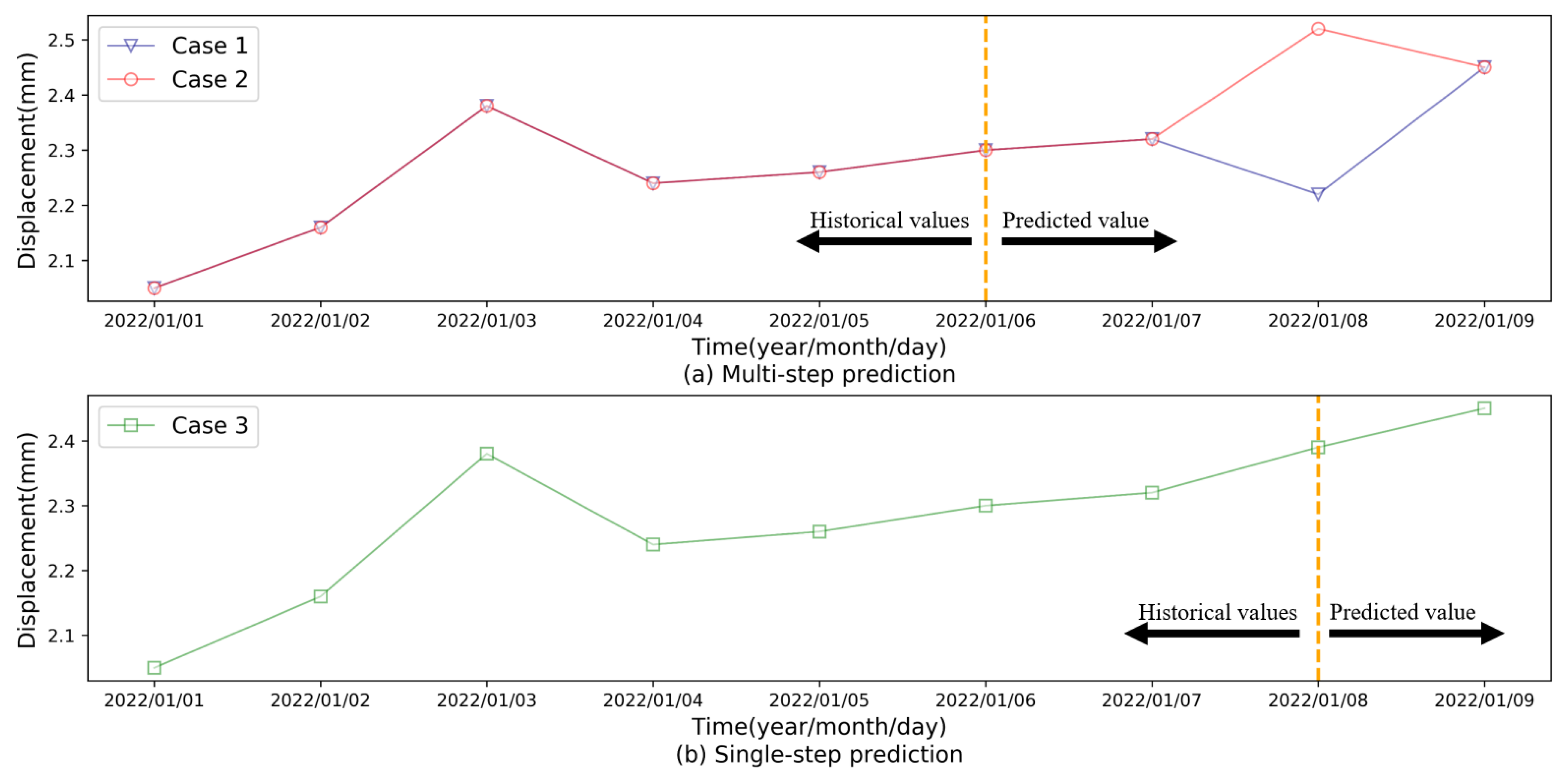
Although the models mentioned above have achieved good prediction results in single value dam displacement monitoring, considering the deformation tendency rather than a given predicted value can better depict the dam’s structural health status, it is of great importance to forecast the evolution of dam displacement in the short term. The multi-step prediction methods provide a means for tendency prediction as they can output multiple results to elaborate on the deformation evolution of dams. To further demonstrate the meaning of multi-step dam displacement predictions, Figure 1 shows a comparison of multi-step and single-step predictions. As we can see in Figure 1, although the multi-step and single-step prediction have the same displacement on 9 January 2022, the single-step result is unable to reflect the variation trend of the deformation among the predicted period. Diverse deformation processes can reflect different structural health statuses even at the same level of displacement. For instance, the last predicted values of Case 1, Case 2, and Case 3 are consistent, while their variation trends are remarkably distinct. Compared to Case 2 and Case 3, Case 1 presents a sharp uptrend, revealing the probable existence of more security risk in Case 1 than in other cases. In this context, capturing the variation trend in the dam displacement in advance can benefit in capturing the behaviors of the dam displacement so as to better ensure dam safety.

Bearing this in mind as motivation, this paper attempts to construct a multi-step prediction model of dam displacement and provide a suitable modeling strategy. Recursive and direct strategies are currently the most common modeling strategies for multi-step prediction. Regarding the recursive strategy, a prediction model is constructed by means of minimizing the squares of the sample one-step-ahead residuals, and the predicted value is used as input for the next prediction [25]. Since the predicted values are used instead of the actual values, the recursive strategy suffers from the error accumulation problem [26,27]. By contrast, researchers proposed the direct strategy method, in which separated models using past observations are constructed for each time step [28,29]. Although the direct strategy can mitigate the cumulative error problem, it is a time-consuming process. To better address these issues, researchers introduced a multiple-input multiple-output (MIMO) strategy. In this multi-target output process, the prediction is performed through a set of vectors, and the size of the vector is equal to the number of forecasting days, which can effectively alleviate the consumption problem of the direct strategy and the error accumulation problem of the recursive strategy. Hence, this paper adopts the MIMO strategy to construct a hybrid model based on the EM-ELM algorithm, namely the CSSKEE model. The model can better predict the short-term dam displacement evolution with excellent predictive accuracy and good generalization performance, thus making dam monitoring more precise and effective.

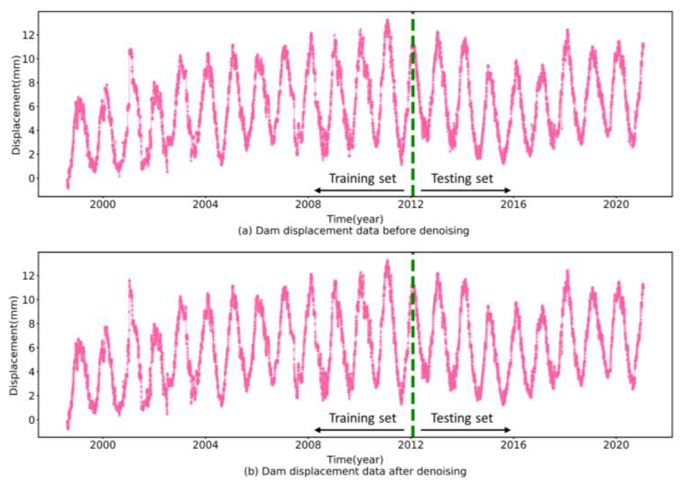
Since uncertainty errors and anomalous data contained in dam displacement data can directly affect the predictive accuracy of the models, signal decomposition techniques have found extensive application in enhancing the predictive accuracy of dam displacement models as they can extract the features of the original data and remove the noise in the original data [30]. The EMD, EEMD, and CEEMD algorithms are three typical signal decomposition techniques [31,32,33]. However, these decomposition techniques suffer from problems such as modal confounding, and energy leakage in the low-frequency region, and other phenomena [34]. In this regard, the complete ensemble empirical mode decomposition with adaptive noise (CEEMDAN) algorithm is proposed by introducing particular noises and computing unique residues which could provide better frequency separation of the extracted sequences. Therefore, this paper uses the CEEMDAN method to decompose the original data and combines other methods, such as the sample entropy method, to eliminate the noise sequence.

Clustering is a search process to excavate possible hidden patterns in data. The clustering method divides the data into several disjoint groups, each of which is similar but different from the other groups [35]. The clustering techniques are applied in fields such as data mining and natural language [36,37,38]. In this paper, clustering analysis is conducted to help identify the features of the short-term variation trend in the dam displacement and to merge similar features. The k-means (KM) algorithm is widely used due to its speed, simple structure, and suitability for regular datasets. However, the clustering results are sensitive to the initial state of the cluster center, making this algorithm prone to falling into local optimal solutions [39,40]. The k-harmonic means (KHM) algorithm is proposed, using the distance of the harmonic mean as a component of the objective to mitigate local optimal issues. To further address this problem, some optimization algorithms have been introduced to enhance the ability of KHM models to obtain the optimal solution. As a novel swarm optimization method, the sparrow search algorithm (SSA) has the superiority of high stability and robustness [41]. Therefore, it is promising to combine the SSA algorithm with the KHM model, and the integrated approach could overcome the shortcoming of falling into the local optimum of the KM algorithm, thus improving the clustering effect as well as the prediction accuracy.

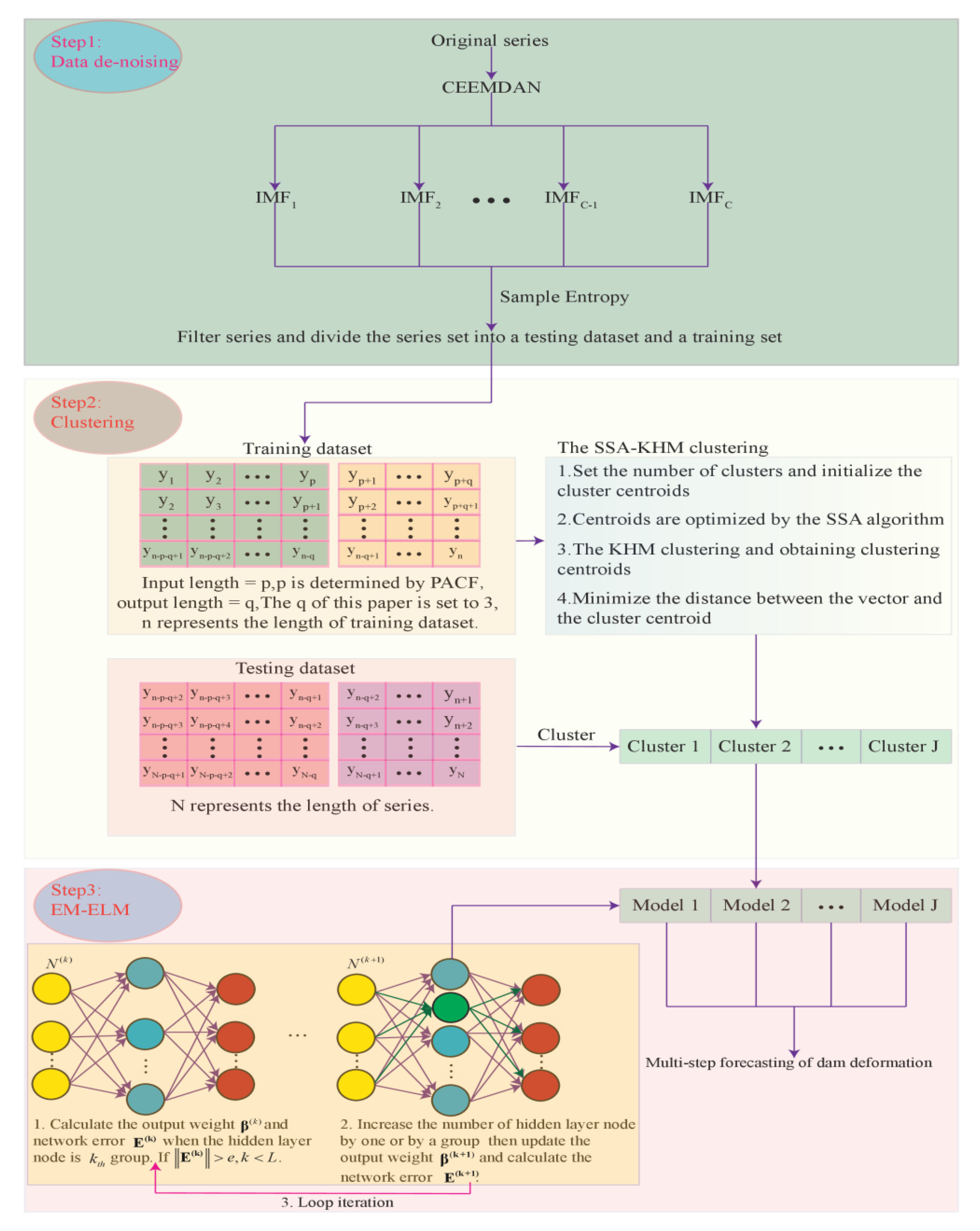
The main contribution of this paper is the proposal of a short-term multi-step prediction method for dam displacement, termed the CSSKEE model. Generally, the model is implemented based on the signal processing method, the computational intelligence algorithm, and multiple machine learning techniques. Firstly, the original data is decomposed by the CEEMDAN model, and the noise is eliminated through counting the sample entropy of decomposed sequences. Secondly, the SSA-KHM algorithm is utilized to cluster the denoised data. Thirdly, the clustered data is finally predicted by the EM-ELM algorithm. Figure 2 shows the specific details of the model. The simulation results confirm that the proposed method can better predict the multi-step dam displacement in the short term.

The remainder of this paper is structured in the following manner. Section 2 introduces the methodology. Then, the effectiveness of the proposed model is elaborated by the case study in Section 3. Finally, the conclusions and future perspectives are outlined in Section 4.

2. Methodology

2.1. Noise Reduction of Prototype Dam Displacement Data

2.1.1. Complete Ensemble Empirical Mode Decomposition with Adaptive Noise

Huang et al. [31] proposed the empirical mode decomposition (EMD) algorithm. As a time-frequency domain processing method, the EMD algorithm can decompose an original signal into a set of intrinsic mode functions (IMFs) and is effective for analyzing nonlinear and nonstationary signals. However, the EMD algorithm has problems such as modal aliasing and significant reconstruction errors [42]. To alleviate this modal aliasing problem, Wu and Huang [32] proposed the ensemble empirical mode decomposition (EEMD) algorithm. In the EEMD algorithm, Gaussian white noise with a zero mean is added for auxiliary analysis. Because of the characteristics of the zero mean, after multiple averaging, the noise will cancel each other, and the final result is the result of the integrated mean. Although the EEMD algorithm has alleviated the modal problem to a certain extent, due to its low decomposition efficiency, problems such as modal aliasing in the low-frequency region and high reconstruction error remain. Yeh et al. [33] developed the complete ensemble empirical mode decomposition (CEEMD) method, which involves adding the positive and negative relative auxiliary white noise to the original signal and phase canceling them in the pooled average, thereby effectively improving the decomposition efficiency and overcoming the problems of large reconstruction error and lack of completeness of the EEMD algorithm. However, there remains a difference in the number of IMFs generated by the CEEMD algorithm during the EMD algorithm decomposition, leading to difficulties in aligning the IMF components in the final ensemble averaging, resulting in an ensemble averaging error. Researchers developed the CEEMDAN algorithm to solve the IMF component alignment problem at ensemble averaging. The CEEMDAN algorithm lowers the noise residual in the final reconstructed signal compared with the CEEMD algorithm result and reduces the screening time. The method also alleviates the problems of difficult alignment of the IMF components due to the differences in the decomposition results and the impact of poor IMF decomposition results on subsequent decomposition sequences. The specific principles can be found in the literature [43].

2.1.2. Sample Entropy

The SE algorithm is derived from approaches developed by [44]. The SE algorithm can be used to measure the complexity of a time series; the higher the entropy value, the higher the sequence complexity and the stronger the randomness; the lower the entropy value, the lower the sequence complexity and the stronger the regularity [45]. The length of the time series $x\left\{x(1),x(2),\cdot \cdot \cdot ,x(n)\right\}$ is set to N. The SE is calculated as follows:

(1) Assume a dimensionality of $m$, the time series can be reconstructed in phase space, yielding the following:

$$x(i)=\left\{x(i),x(i+1),\cdot \cdot \cdot ,x(i+m-1)\right\}$$

(1)

Here, $i=1,2,\cdot \cdot \cdot ,\mathrm{N}-m+1$.

(2) Calculate the maximum difference between the corresponding elements of $x(i)$ and $x(j)$, the following formula for details:

$$d[x(i),x(j)]=\underset{k\in (0,m-1)}{\max }\left|x(i+k)-x(j+k)\right|$$

(2)

(3) Assume a $r$$\left(r>0\right)$, for each $1\le i,j\le N-m$, calculate the ratio of the number of $d[x(i),x(j)]<r$ to the total number of vectors $\mathrm{N}-m-1$, as follows:

$${\mathrm{B}}_i^m(r)=\frac{1}{\mathrm{N}-m-1}num\left\{d[x(i),x(j)]<r\right\}$$

(3)

(4) Average all the results obtained from Step (3), as follows:

$${\mathrm{B}}^m(r)=\frac{1}{\mathrm{N}-m}{\displaystyle \sum _{i=1}^{\mathrm{N}-m}{\mathrm{B}}_i^m(r)}$$

(4)

(5) Repeat steps (1)–(4) for the $m+1$ dimensional vector to obtain $G^m(r)$, and calculate SE:

$$SampEn(m,r,\mathrm{N})=-\ln \left[\frac{G^m(r)}{B^m(r)}\right]$$

(5)

In this paper, to reconstruct the original data, we decompose the original sequence by the CEEMDAN algorithm, then calculate SE algorithm of each subsequence, and finally determine whether the subsequence is a noisy sequence according to the size of the sample entropy algorithm so as to reconstruct the original data. In addition, another evaluation index has been employed to verify the selection of noisy sequences, and the index is defined as follows:

• Denote the length of the dam deformation sequence $x\left\{x(1),x(2),\cdot \cdot \cdot ,x(n)\right\}$ to N. Then $x$ is decomposed and can be expressed as:

  $$x(n)={\displaystyle \sum _{i=1}^{D}IM{F}_i(n)}+r(n)$$

  (6)

  where $D$ is the number of decomposed IMFs; ${\mathrm{IMF}}_i(n)$ is the decomposed subsequence; $r(n)$ is the residual series.
• Define the c-filtering reconstruction $y_c(n)$ as

  $$y_c(n)={\displaystyle \sum _{i=c}^{D}IM{F}_i(n)}+r_D(n)$$

  (7)

  where $c=1,2,\cdot \cdot \cdot ,D$; $r_D(n)$ is the residual series.
• Eliminate the IMF by taking the minimum value from the following equation

  $$\mathrm{SMSE}\left(y_c(n),y_{c+1}(n)\right)=\frac{1}{\mathrm{N}}{\displaystyle \sum _{n=1}^{\mathrm{N}}{[y_c(n)-y_{c+1}(n)]}^2}=\frac{1}{\mathrm{N}}{\displaystyle \sum _{n=1}^{\mathrm{N}}[IM{F}_c}(n){]}^2$$

  (8)

  where $c=1,2,\cdot \cdot \cdot ,D-1$.

2.2. Clustering

2.2.1. K-Harmonic Means

To overcome the problem that the k-means algorithm easily falls into the local optimal solution, for each data object in the dataset, the KHM uses the sum of the harmonic means of the data to all the cluster centers, and the affiliation function and particle weights are used to update the cluster centers. The harmonized mean sum of all data is used as the evaluation index. The specific process of the KHM clustering algorithm is shown below [46].

1. Select $k$ initial centroids $c_1,c_2,\cdot \cdot \cdot ,c_k$ randomly, where $c_k$ is the centroid of the $k_{th}$ cluster, set $t$ to the number of iterations.

2. Calculate the fitness function:

$$F\left(X,c_1,c_2,\cdot \cdot \cdot ,c_k\right)={\displaystyle \sum _{i=1}^{\mathrm{n}}\frac{j}{{\displaystyle \sum _{k=1}^K\frac{1}{{‖x_i-c_k‖}^p}}}}$$

(9)

In the formula: $X=\left\{x_1,x_2,\cdot \cdot \cdot ,x_n\right\}$, $n$ is the number of objects to be clustered, $p$ is an input parameter Generally $p\ge 2$.

3. For $x_i$ calculate its affiliation at each center $c_k$:

$$m(c_k\left|x_i\right.)=\frac{{‖x_i-c_k‖}^{-p-2}}{{\displaystyle \sum _{k=1}^K{‖x_i-c_k‖}^{-p-2}}}$$

(10)

4. For $x_i$, calculate its weight:

$$w(x_i)=\frac{{\displaystyle \sum _{k=1}^K{‖x_i-c_k‖}^{-p-2}}}{{\left({\displaystyle \sum _{k=1}^K{‖x_i-c_k‖}^{-p}}\right)}^2}$$

(11)

5. For $c_k$, recalculate the clustering centers based on their affiliation, weights, and all data points $x_i$:

$$c_k=\frac{{\displaystyle \sum _{i=1}^{n}m(c_k\left|x_i\right.)w(x_i)x_i}}{{\displaystyle \sum _{i=1}^{n}m(c_k\left|x_i\right.)w(x_i)}}$$

(12)

6. Repeat 2–5 until the set number of iterations is exceeded:

7. Classify sample $x_i$ into the largest group $k$ of $m(c_k\left|x_i\right.).$

2.2.2. Sparrow Search Algorithm

The SSA algorithm is a heuristic optimization algorithm. The algorithm consists of followers, discoverers, and investigators [47]. The guidelines followed by the SSA algorithm are as follows:

Assuming that the parameter being searched is 1d data, a group of $n$ sparrows can be expressed by the following formula:

$$X=\left[\begin{array}{l}{x}_1^1 x_1^2 \dots x_1^d\\ x_2^1 x_2^2 \dots x_2^d\\ \dots \dots \dots \dots \\ x_n^1 x_n^2 \dots x_n^d\end{array}\right]$$

(13)

Here, $d$ is the number of dimensions, and $n$ is the number of sparrows. The fitness of the sparrow is expressed by Equation (14):

$$F_x=\left[\begin{array}{l} f\left(\left[x_1^1{x}_1^2\dots x_1^d\right]\right)\\ f\left(\left[x_2^1{x}_2^2\dots x_2^d\right]\right)\\ \dots f\left(\left[x_n^1{x}_n^2\dots x_n^d\right]\right)\end{array}\right]$$

(14)

Here, $f$ denotes the adaptation value.

For sparrow colonies, a discoverer with better adaptability provide an important resource for the entire colony and guide the predation direction of other sparrows in their predation:

$$X_{i,j}^{t+1}=\left\{\begin{array}{l}{X}_{i,j}^t\cdot \exp \left(-\frac{i}{\theta \cdot ite{r}_{\max }}\right),if Q_2<ZD\\ X_{i,j}^t+R\cdot T,if Q_2\ge ZD\end{array}\right.$$

(15)

Here, $X_{i,j}$ represents the position information of the $i_{th}$ sparrow in the $j_{th}$ dimension. $t$ represents the current number of iterations, $j=1,2,3,\cdot \cdot \cdot ,d.$ $ite{r}_{\max }$ represents the maximum number of iterations. $\theta \in \left(0,1\right]$ is a random number. $R$ stands for a random number that follows a normal distribution. $T$ represents a $1\times d$ matrix with an element of 1. $Q_2\left(Q_2\in \left[0,1\right]\right)$ and $ZD\left(ZD\in \left[0.5,1\right]\right)$ indicate the alarm and safety values, respectively.

When $Q_2<ZD$, it indicates that no aggressor is found around the predation area, and the discoverer is able to perform an extensive search mechanism. If $Q_2\ge ZD$, representing individuals in the group to spot the aggressor and sound the alarm, all individuals in the group take anti-predation behavior, and the discoverer will take the follower to a relatively safe position [48]. The position of the follower is updated as shown in the following equation:

$$X_{i,j}^{t+1}=\left\{\begin{array}{l}R\cdot \exp \left(\frac{X_{ws}^t-X_{i,j}^t}{i^2}\right),if i>n/2\\ X_p^{t+1}+\left|X_{i,j}^t-X_p^{t+1}\right|\cdot A^{+}\cdot T, \mathrm{otherwise}\end{array}\right.$$

(16)

$$A^{+}=A^T{(A{A}^T)}^{-1}$$

(17)

Here, $X_{ws}$ represents the current global worst position and $X_p$ represents the best position occupied by the discoverer. $A$ represents $1\times d$ matrix with a random value of 1 or −1. When $i>n/2$, it indicates that the $i_{th}$ follower is in a position where there is less food and needs to go to a location where food is abundant.

Sparrow colonies will defend themselves when they feel dangerous. The investigators were randomly selected individuals from the sparrow population. When predators appear in the vicinity of the population, they will promptly alert the entire population regarding the anti-predatory behavior, and the mathematical expression is as follows:

$$X_{i,j}^{t+1}=\left\{\begin{array}{l}{X}_{bs}^t+\delta \cdot \left|X_{i,j}^t-X_{bs}^t\right|,if f_i>f_g\\ X_{i,t}^t+M\cdot \left(\frac{\left|X_{i,j}^t-X_{ws}^t\right|}{\left(f_i-f_w\right)+\alpha }\right),if f_i=f_g\end{array}\right.$$

(18)

Here $X_{bs}$ represents the current global best position. $\delta$ represents a random number that follows a standard normal distribution. $\alpha$ represents a very small constant. $M\in \left[-1,1\right]$ represents a random number. $f_i$ indicates the adaptation value of the current sparrow. $f_w$ and $f_g$ represent the current global worst fitness and optimal fit, respectively. When $f_i>f_g$, it means that the sparrow is on the edge of the population. When $f_i=f_g$, it means that the sparrows in the middle of the group are aware of the danger and need to approach the other sparrows to avoid the danger. The process is shown below:

Step 1: Initialize the number of discoverers, followers, investigators, and iterations.

Step 2: Calculate the fitness values of all the sparrows to rank and find the best and worst individuals.

Step 3: Update the discoverer location using Equation (15).

Step 4: Update the follower positions using Equations (16) and (17).

Step 5: Update the investigator positions using Equation (18).

Step 6: If the optimal sparrow fitness is inferior to the updated sparrow fitness, the optimal fitness is updated.

Step 7: Determine whether the number of iterations exceeds the maximum number of iterations. If satisfied, the program is terminated and the final result is output, otherwise, the execution of steps 2–6 is repeated.

2.2.3. SSA-KHM Algorithm Flow

Since the KHM algorithm has a more straightforward structure than the SSA algorithm, it converges faster; however, it typically falls into local optimum solutions. To overcome the local optimum issue, this study uses a hybrid model comprising the SSA and KHM algorithms to determine the clustering centers. The model can maintain the advantages of the KHM and SSA algorithms to better cluster the data and capture the characteristics of the data in the time series, enabling a more accurate multi-step prediction of the dam deformation data. The specific flow of the SSA-KHM model is shown below:

• Divide the dam deformation data into a 60% training set and a 40% test set and normalize. The training set is clustered, and its cluster centers are calculated, and the test set is clustered using the cluster centers of the training set.
• Initialize the cluster center and set the maximum number of iterations $Iter\max$.
• Set $G_1=0$.
• Set $G_2=G_3=0$.
• The SSA method

  5.1

  Use the SSA algorithm to update the clustering center.

  5.2

  $G_2=G_2+1$. If $G_2<3$, then return to 5.1.

• The KHM method

  6.1

  The current location of the individual is used as the initial cluster center and updated by the KHM algorithm.

  6.2

  $G_3=G_3+1$. If $G_3<7$, then return to 6.1.

• $G_1=G_1+1$. If $G_1<Iter\max$, then return to 4.
• Classify sample $x_i$ into the largest group $k$ of $m(c_k\left|x_i\right.).$

2.3. Prediction

2.3.1. Extreme Learning Machine

Conventional neural network learning algorithms require setting a large number of artificial network training parameters [49]. By contrast, the extreme learning machine (ELM) algorithm can randomly initialize input weights, biases, and the number of hidden layer nodes and obtain the corresponding output weights by least squares. The entire learning is performed by a mathematical change without any iterations, which makes the ELM algorithm a compact yet effective learning algorithm [50]. The ELM algorithm process is as follows:

$${\displaystyle \sum _{i=1}^L{\beta }_{i}g\left(W_i\cdot X_j+b_i\right)}={\stackrel{\sim }{y}}_j,j=1,\cdot \cdot \cdot ,N$$

(19)

Here, $g\left(x\right)$ is the activation function ($sigmoid$ is chosen as the activation function in this paper), $W_i$ is the input weight, $b_i$ denotes the bias of the $i_{th}$ hidden layer cell, and ${\beta }_i$ indicates the output weights. In order to obtain ${\beta }_i$ with good results using the training sample set, the goal of the ELM algorithm is to minimize the error of the output:

$${\displaystyle \sum _{j=1}^N‖{\stackrel{\sim }{y}}_j-t_j‖}=0$$

(20)

There exists ${\beta }_i$, $W_i$, and $b_i$, which makes:

$${\displaystyle \sum _{i=1}^L{\beta }_{i}g\left(W_i\cdot X_j+b_i\right)}=t_j,j=1,\cdot \cdot \cdot ,N$$

(21)

Equation (21) can be expressed as:

$$H\beta =T$$

(22)

Here, $T$ represents the desired output, $\beta$ represents the output weight, and $H$ represents the output of the hidden node.

The output weight $\beta$ can be determined by Equation (23):

$$\mathit{\beta }={\mathit{H}}^{†}\mathit{T}={\left({\mathit{H}}^{\mathit{T}}\mathit{H}\right)}^{-1}{\mathit{H}}^{\mathit{T}}\mathit{T}$$

(23)

Here, $H^{†}$ is the Moore–Penrose generalized inverse of the matrix $H$ and the norm of $\beta$ is minimal and unique.

2.3.2. Error Minimized Extreme Learning Machine (EM-ELM)

Although the structure of the ELM algorithm is simple and effective, choosing the optimal number of hidden layer nodes remains problematic. In contrast, the EM-ELM algorithm can add hidden nodes individually or in batches; the output weight value is updated each time a new hidden node is added, which reduces the computational complexity. Generally, the EM-ELM algorithm can be divided into two steps: initialization and learning. In the initialization phase, the initial network structure is constructed by giving an initial number of hidden layer nodes, and the initial hidden layer output matrix and initial residual error $\epsilon >0$ are calculated. In the learning phase, hidden nodes are added individually or in batches, the hidden output matrix is calculated, and the output weights and residual errors are updated. The specific flow of the EM-ELM algorithm is as follows:

Suppose $N$ arbitrary samples $\left(X_i,t_i\right)\in R^n\times R^m(i=1,2,\cdot \cdot \cdot ,N)$, the maximum number of hidden layer nodes is $L_{\max }$, initial hidden layer node $L_0$, and hidden layer activation function $g\left(x\right)$.

Initialization phase:

(1) Initial hidden layer node $L_0$ randomly generates initial weights and biases ${(W_i,b_i)}_{i=1}^{L_0}.$

(2) Calculate the initial hidden layer output matrix $H_0$ according to Equation (24).

$$H_0={\left[\begin{array}{l}g(w_1,b_1,x_1) \dots g(w_{L_0},b_{L_0},x_1)\\ ⋮ ⋮\\ g(w_1,b_1,x_N) \dots g(w_{L_0},b_{L_0},x_N)\end{array}\right]}_{N\times L_0}$$

(24)

(3) Calculate the initial residual output error according to Equation (25).

$$E_0=‖H_0{H}_0^{{}^{†}}T-T‖$$

(25)

Learning phase:

(1) $k=0$, while $L_k<L_{\max }$ and $E_k>\epsilon$ (1) $k=k+1$.

(2) Randomly generate $\mathrm{\Delta }{L}_{k-1}$ nodes to add to the existing network. At this time $L_k=L_{k-1}+\mathrm{\Delta }{L}_{k-1}$, and the hidden layer output matrix $H_k=\left[H_{k-1},\mathrm{\Delta }{H}_{\mathrm{\Delta }{L}_{k-1}}\right]$, where:

$$\mathrm{\Delta }{H}_{\mathrm{\Delta }{L}_{k-1}}={\left[\begin{array}{l}g(w_{L_{k-1}}+1,b_{L_{k-1}}+1,x_1) \dots g(w_{L_k},b_{L_k},x_1)\\ ⋮ ⋮\\ g(w_{L_{k-1}}+1,b_{L_{k-1}}+1,x_N)\dots g(w_{L_k},b_{L_k},x_N)\end{array}\right]}_{N\times N_{k-1}}$$

(26)

Equations (27)–(29) are used to calculate the output weights.

$${\mathit{D}}_{\mathit{k}}=\left(\right(\mathit{I}-{\mathit{H}}_{\mathit{k}-1}{\mathit{H}}_{\mathit{k}-1}^{†})\mathrm{\Delta }{\mathit{H}}_{\mathit{\Delta }{\mathit{L}}_{\mathit{k}-1}}{)}^{†}$$

(27)

$${\mathit{U}}_{\mathit{k}}={\mathit{H}}_{\mathit{k}-1}^{†}(\mathit{I}-\mathrm{\Delta }{\mathit{H}}_{\mathit{\Delta }{\mathit{L}}_{\mathit{k}-1}}^{\mathit{T}}{\mathit{D}}_{\mathit{k}})$$

(28)

$${\beta }_k=H_k^{†}T=\left[\begin{array}{l}{U}_k\\ D_k\end{array}\right]T$$

(29)

End While.

3. Case Study

A case study was conducted on a concrete dam located in China with a height of 63 m, a crest length of 196.62 m, a left bank width of 8 m, a right bank width of 6 m, and a bottom width of 46.5 m. The main structures include a barrage, a water diversion system, a powerhouse, and a switching station. The dam was put into storage in 1993 and passed completion acceptance in 1995. To better ensure the safe operation of the dam, in August 2000, renovation of the automated system was conducted for automatic monitoring of the deformation. A lead line was placed at the top of the dam to monitor the horizontal displacement of the dam, with a total of seven points, numbered E01–E07. In addition, there is an inverted plumb line at each end of the lead wire to monitor the horizontal displacement, numbered IP1 and IP2. The data were acquired once a day, and the layout scheme is shown in Figure 3.

In this study, the radial displacement at the monitoring point E04 in the overflow section of the dam was selected as the test case (negative toward upstream and positive toward downstream). The E04 dataset was created between August 1998 and January 2021, and the first 60% of the data was selected for model training, and the rest of the data was used as the test set to verify the prediction performance of the model. Mean absolute error (MAE) and root mean square error (RMSE) are used to evaluate the predictive accuracy. See the following formula for details:

$$MAE=\frac{1}{a}{\displaystyle \sum _{i=1}^a\left|y_i-\stackrel{\sim }{y_i}\right|}$$

(30)

$$MSE=\frac{1}{a}{{\displaystyle \sum _{i=1}^a\left(y_i-\stackrel{\sim }{y_i}\right)}}^2$$

(31)

where $a$ is the number of samples; $y_i$ is the measured value of the dam’s displacement; and ${\stackrel{\sim }{y}}_i$ is the predicted value of the dam’s displacement.

3.1. Denoising of Prototype Dam Displacement Data

In this study, the prototype dam displacement data were denoised using the method proposed in Section 2.1. The implemented process is as follows:

Step 1: Divide the data into 60% training sets and 40% testing sets.

Step 2: Use the CEEMDAN to decompose the training set data, and then the method introduced in Section 2.1.2 is utilized to judge which of the decomposed IMF sequences are noisy sequences and remove them.

Step 3: The displacement data are denoised and reconstructed according to the calculation results of the training set.

Figure 4 exhibits the decomposition results of the E04 test set deformation, and the calculated sample entropy and the SMSE values of IMFs are listed in

Table 1. Sample entropy values of IMFs.

Subsequences	Imf1	Imf2	Imf3	Imf4	Imf5	Imf6	Imf7	Imf8	Imf9
entropy	1.0518	0.8186	0.6306	0.5638	0.3276	0.0669	0.0232	0.0086	9.7 × 10−5

and

Table 2. SMSE values of IMFs.

Subsequences	Imf1	Imf2	Imf3	Imf4	Imf5	Imf6	Imf7	Imf8	Imf9
SMSE	0.0248	0.0419	0.0622	0.0771	0.1812	7.1408	0.1217	0.0296	36.8884

. The magnitude of the sample entropy and the SMSE values can measure the complexity of IMFs. When the sample entropy value is large and the SMSE value is small, the corresponding IMFs sequence is determined as a noise sequence. Accordingly, IMF1 is identified as a noise sequence and eliminated. Moreover, to verify the applicability of the proposed denoising method, the deformation sequences before and after denoising are plotted in Figure 5. As shown in Figure 5, the denoised sequence trends are generally consistent with the original sequence while having a higher smoothness, which reveals that the proposed denoising method can better remove the redundant information while preserving the original sequence features.

3.2. Prediction Results Based on EM-ELM, LSTM and CNN before and after Denoising Displacement Data

Since the partial autocorrelation function (PACF) is a statistical method that directly describes the relationship between time series and their lags, PACF can verify the time correlation of a sequence. Therefore, PACF is utilized to consider the influence of dam deformation self-sequential lag on dam displacement in this paper. Figure 6 plots the PACF before and after denoising. According to Figure 6 (the shaded area is the 95% confidence interval), the PACF of the prototype dam displacement data before denoising presents a 39th order truncation; accordingly, the data input length before denoising is adopted as 39. Similarly, the data input length after denoising is chosen as 4. The results before and after denoising the data are further analyzed and compared using EM-ELM, LSTM, and CNN models. The indicators of the six models are listed in

Table 3. Performance comparison of different algorithms on the test set (predicted three-day average).

Algorithm	CS-EMELM	EMELM	CS-LSTM	LSTM	CS-CNN	CNN
RMSE (mm)	0.2235	0.6602	0.2504	0.3314	0.2707	0.6376
MAE (mm)	0.1419	0.4920	0.1706	0.2314	0.1894	0.5180
Time(s)	60.87	53.28	89.66	193.67	72.64	94.70

Note: The best results are highlighted in boldface.

,

Table 4. Comparison of RMSE of different algorithm test set for different prediction days.

	Algorithm	CS-EMELM	EMELM	CS-LSTM	LSTM	CS-CNN	CNN
Prediction Days
First day (mm)		0.0714	0.6207	0.1026	0.2358	0.1241	0.6086
Second day (mm)		0.1969	0.6609	0.2307	0.3315	0.2551	0.6319
Third day (mm)		0.3256	0.6967	0.3526	0.4049	0.3733	0.6709

Note: The best results are highlighted in boldface.

and

Table 5. Comparison of MAE of different algorithm test set for different prediction days.

	Algorithm	CS-EMELM	EMELM	CS-LSTM	LSTM	CS-CNN	CNN
Prediction Days
First day (mm)		0.0478	0.4598	0.0716	0.1532	0.0934	0.4951
Second day (mm)		0.1388	0.4932	0.1719	0.2382	0.1916	0.5131
Third day (mm)		0.2391	0.5229	0.2683	0.3027	0.2833	0.5458

Note: The best results are highlighted in boldface.

, and Figure 7 shows the residual distribution of each model.

In order to intuitively verify the effectiveness of the denoising method proposed in this paper, a comparative analysis of the results listed in Table 3 is performed. The results show that, after denoising the prototype dam displacement sequence, the RMSE and MAE of the EM-ELM algorithm on the test set are improved by 66.15% and 71.16%, respectively. The RMSE and MAE of the LSTM algorithm on the test set are improved by 24.44% and 26.27%, respectively. The RMSE and MAE of the CNN algorithm on the test set are improved by 57.54% and 63.44%, respectively. In summary, the accuracy of the multi-step predictive model can be improved by using the denoising sequence, which suggests that the proposed denoising method can effectively remove redundancy information from the data and thereby increase the prediction accuracy.

Furthermore, the statistical indicators in Table 3 are analyzed to verify the applicability and validity of each prediction model. From Table 3, in comparison to the CNN algorithm, the LSTM algorithm improves the RMSE and MAE on the test set by 48.02% and 55.33%, respectively, while the time performance decreases by 51.10%. Compared with the EM-ELM algorithm, the LSTM algorithm improves the RMSE and MAE on the test set by 49.80% and 52.97%, respectively, while the time performance decreases by 72.49%. Regarding the prediction performance after denoising, the CS-EMELM algorithm improves the RMSE and MAE on the test set by 10.74% and 16.82% compared with the CS-LSTM algorithm, respectively, and the time performance improves by 32.11%. With respect to the CS-CNN algorithm, the CS-EMELM algorithm improves the RMSE and MAE on the test set by 17.44% and 25.08%, respectively, and the time performance improves by 16.20%. To summarize the above, without any special denoise processing, the LSTM algorithm illustrates stronger generalization ability compared with CNN and EMELM algorithms, which shows that the LSTM algorithm is capable of capturing the temporal characteristics contained in noise sequences and results in better prediction ability for the redundant prototype data. After denoising the data through the CS algorithm, the performance of all involved approaches has been improved to a large extent, especially the EM-ELM algorithm, which achieves the most significant improvement and results in similar predictive accuracy with the other two models, which demonstrates that by incorporating the CS algorithm, the EM-ELM algorithm can capture and reveal the temporal characteristics of the data and has great predictive accuracy. Moreover, to obtain a reasonable solution, the implementation of LSTM and CNN algorithms is usually complicated, dueto the need to employ optimization algorithms to determine multiple hyperparameters. Hence, taking advantage of combining good accuracy with an affordable computational cost, the CS-EMELM algorithm is utilized as the predictive model in the proposed method.

The prediction results of all involved models under different forecasting days are shown in Figure 8, Figure 9 and Figure 10, and the values of the evaluation criteria are given in Table 4 and Table 5. In comparison to the second-day predicted value, the first-day predicted value of the CS-EMELM algorithm improves by 63.74% and 65.56% in RMSE and MAE, respectively; the first-day predicted value of the CS-LSTM algorithm improves by 55.53% and 58.35% in RMSE and MAE, respectively. The first-day predicted value of the CS-CNN algorithm improves by 51.35% and 51.25% in RMSE and MAE, respectively. Compared with the third-day predicted value, the second-day predicted value of the CS-EMELM algorithm improves by 39.53% and 41.95% in RMSE and MAE, respectively, the second-day predicted value of the CS-LSTM algorithm improves by 34.57% and 35.93% in RMSE and MAE, respectively, the second-day predicted value of the CS-CNN algorithm improves by 31.66% and 32.37% in RMSE and MAE, respectively. In general, since the generalization ability of the model deteriorates as the forecasting duration increases and the short-lag feature of dam displacement data increases, the models’ predictive accuracy decreases with the increase in the predictive period.

3.3. Prediction Analysis after Clustering

The short-term variation trend of the dam displacement sequence may contain similar characteristics in different periods. The grouping of data into classes or clusters is a process of data clustering, which can make the data in each cluster highly similar while being very dissimilar to data from other clusters. As the data feature in each group is concentrated after the clustering process, better performance can be achieved by implementing the predicting methods for each group separately. As mentioned in Section 2.2.3, the SSA-KHM model can better overcome the shortcomings of traditional clustering models, which are sensitive to the initial clustering center, and thus improve the accuracy of clustering. Consequently, this paper uses the SSA-KHM model to cluster the data. Notably, the choice of the clustering number may affect the accuracy of the SSA-KHM model. TO address this problem, researchers have proposed some criteria to determine the optimal number of clusters. Nevertheless, the effectiveness of these criteria for dam displacement clustering is still unclear, particularly for the clustering problem of dams’ multi-step displacement prediction. In this paper, the optimal number of clusters is determined using the traversal method [51].

Figure 11 and Figure 12 plot the distribution of the datasets after clustering. The results show that the grouped sub-datasets are distributed around their respective clustering centers, indicating that the proposed method can effectively extract the different characteristics contained in the sequence and precisely cluster data with the same characteristics.

Table 6. Performance comparison of different number of clusters on the test set.

Number of Clusters	K = 1	K = 2	K = 3	K = 4	K = 5	K = 6	K = 7	K = 8
RMSE	0.2235	0.2237	0.2215	0.2268	0.2256	0.2261	0.2242	0.2260
MAE	0.1419	0.1444	0.1417	0.1444	0.1434	0.1447	0.1426	0.1423

Note: The best results are highlighted in boldface.

demonstrates the prediction results under different classifications. As shown in Table 6, the optimal number of clusters is acquired by quantifying the statistical indicators, and the model constructed by three clusters provides better fitting performance than the model constructed by the other clustering numbers. Nevertheless, the deformation characteristics of gravity dams are less complicated due to their relatively simple structural forms and stable operating state. Therefore, fewer features of dam deformation can be extracted by clustering methods, which results in a mild improvement in the prediction accuracy. In view of the above, the proposed method can be further applied to other hydraulic structures, such as earth-rock dams, and arch dams where more complex deformation characteristics are present.

By analyzing the metrics in

Table 7. Comparison of RMSE for different number of clusters for different days of prediction on the test set.

	Group	K = 1	K = 2	K = 3	K = 4	K = 5	K = 6	K = 7	K = 8
Prediction Days
First day (mm)		0.0714	0.0762	0.0712	0.0750	0.0735	0.0743	0.0763	0.0742
Second day (mm)		0.1969	0.1975	0.1946	0.2006	0.1989	0.1992	0.1982	0.2002
Third day (mm)		0.3256	0.3246	0.3230	0.3293	0.3281	0.3289	0.3251	0.3281

Note: The best results are highlighted in boldface.

and

Table 8. Comparison of MAE for different number of clusters for different days of prediction on the test set.

	Group	K = 1	K = 2	K = 3	K = 4	K = 5	K = 6	K = 7	K = 8
Prediction Days
First day (mm)		0.0478	0.0524	0.0475	0.0495	0.0491	0.0506	0.0508	0.0490
Second day (mm)		0.1388	0.1406	0.1384	0.1414	0.1402	0.1411	0.1385	0.1391
Third day (mm)		0.2391	0.2400	0.2391	0.2422	0.2409	0.2423	0.2385	0.2388

Note: The best results are highlighted in boldface.

, and Figure 13, the effects of different cluster numbers for different prediction days can be obtained. When taking K = 3 (the optimal number), the predicting accuracy of the model outperforms other scenarios with various clustering numbers within different forecast days. Meanwhile, as the number of prediction days increases, the prediction accuracy of the proposed model can be remarkably enhanced when the optimal clustering number is adopted.

4. Discussion

The model proposed in this paper is based on statistical methods and only considers displacement values as input variables. Some explicitly influential factors, such as temperature, water level, etc., which are well-established in physics, are not directly considered input factors in the proposed model. Incorporating these factors directly into the model as inputs using existing analysis methods may lead to a decrease in predictive accuracy due to accumulated measurement errors in the environmental factor measurement devices. Therefore, in future research, how to integrate these environmental factors and propose efficient and accurate predictive modeling approaches will further enhance the physical interpretability of the model and improve its applicability.

5. Conclusions

In this paper, a multi-step hybrid prediction model is established, aiming to accurately capture the variation trend in the short-term deformation of concrete dams, which is simplified into the CSSKEE model. The model is applied to the displacement prediction of a dam in China, and the experimental results show that it can effectively predict the dam deformation variation trend so as to reflect the resulting structural behavior induced by the deformation variation, thus better ensuring the safety of dam operation. The main conclusions of this work are summarized below:

(1)

The CEEMDAN and SE methods can effectively distinguish the noise term and characteristic term of the measured deformation sequence, which can remove the redundancy of the prototype dam displacement sequence effectively and efficiently.

(2)

The SSA algorithm can better solve the local-trapped problem by applying the KHM method to clustering problems, which achieves better clustering results of the sequence and improves the accuracy of the prediction model.

(3)

The CSSKEE method proposed in this paper achieves the estimation of dam deformation trends by performing multi-step predictions on dam deformation. Compared to traditional single-step prediction methods, this approach elevates the prediction of a single measurement value to the prediction of deformation trends using multiple measurement values. As a result, it can better reflect future changes in the safety status of the dam, effectively enriching and expanding the theory and methods of dam safety monitoring.

References

1. Liu, B.; Wei, B.; Li, H.; Mao, Y. Multipoint hybrid model for RCC arch dam displacement health monitoring considering construction interface and its seepage. Appl. Math. Model. 2022, 110, 674–697. [Google Scholar] [CrossRef]
2. Su, H.; Li, X.; Yang, B.; Wen, Z. Wavelet support vector machine-based prediction model of dam deformation. Mech. Syst. Signal Process. 2018, 110, 412–427. [Google Scholar] [CrossRef]
3. Stojanovic, B.; Milivojevic, M.; Ivanovic, M.; Milivojevic, N.; Divac, D. Adaptive system for dam behavior modeling based on linear regression and genetic algorithms. Adv. Eng. Softw. 2013, 65, 182–190. [Google Scholar] [CrossRef]
4. Kang, F.; Liu, J.; Li, J.; Li, S. Concrete dam deformation prediction model for health monitoring based on extreme learning machine. Struct. Control Health Monit. 2017, 24, 1997. [Google Scholar] [CrossRef]
5. Ardito, R.; Cocchetti, G. Statistical approach to damage diagnosis of concrete dams by radar monitoring: Formulation and a pseudo-experimental test. Eng. Struct. 2006, 28, 2036–2045. [Google Scholar] [CrossRef]
6. Szostak-Chrzanowski, A.; Chrzanowski, A.; Massiéra, M. Use of deformation monitoring results in solving geomechanical problems—Case studies. Eng. Geol. 2005, 79, 3–12. [Google Scholar] [CrossRef]
7. Ren, Q.; Li, M.; Song, L.; Liu, H. An optimized combination prediction model for concrete dam deformation considering quantitative evaluation and hysteresis correction. Adv. Eng. Inform. 2020, 46, 101154. [Google Scholar] [CrossRef]
8. Cao, W.; Wen, Z.; Su, H. Spatiotemporal clustering analysis and zonal prediction model for deformation behavior of super-high arch dams. Expert Syst. Appl. 2022, 216, 119439. [Google Scholar] [CrossRef]
9. Chen, S.; Gu, C.; Lin, C.; Hariri-Ardebili, M.A. Prediction of arch dam deformation via correlated multi-target stacking. Appl. Math. Model. 2021, 91, 1175–1193. [Google Scholar] [CrossRef]
10. Wen, Z.; Zhou, R.; Su, H. MR and stacked GRUs neural network combined model and its application for deformation prediction of concrete dam. Expert Syst. Appl. 2022, 201, 117272. [Google Scholar] [CrossRef]
11. Lin, C.; Wang, X.; Su, Y.; Zhang, T.; Lin, C. Deformation Forecasting of Pulp-Masonry Arch Dams via a Hybrid Model Based on CEEMDAN Considering the Lag of Influencing Factors. J. Struct. Eng. 2022, 148, 04022078. [Google Scholar] [CrossRef]
12. Qu, X.; Yang, J.; Chang, M. A deep learning model for concrete dam deformation prediction based on RS-LSTM. J. Sens. 2019, 2019, 4581672. [Google Scholar] [CrossRef]
13. Dai, B.; Gu, C.; Zhao, E.; Qin, X. Statistical model optimized random forest regression model for concrete dam deformation monitoring. Struct. Control. Health Monit. 2018, 25, e2170. [Google Scholar] [CrossRef]
14. Su, Y.; Weng, K.; Lin, C.; Chen, Z. Dam Deformation Interpretation and Prediction Based on a Long Short-Term Memory Model Coupled with an Attention Mechanism. Appl. Sci. 2021, 11, 6625. [Google Scholar] [CrossRef]
15. Kao, C.Y.; Loh, C.H. Monitoring of long-term static deformation data of Fei-Tsui arch dam using artificial neural network-based approaches. Struct. Control. Health Monit. 2013, 20, 282–303. [Google Scholar] [CrossRef]
16. Gourine, B.; Khelifa, S. Analysis of Dam Deformation Using Artificial Neural Networks Methods and Singular Spectrum Analysis. In Proceedings of the Euro-Mediterranean Conference for Environmental Integration, Sousse, Tunisia, 22–25 November 2017; Springer: Cham, Switzerland, 2017; pp. 871–874. [Google Scholar] [CrossRef]
17. Liu, W.; Pan, J.; Ren, Y.; Wu, Z.; Wang, J. Coupling prediction model for long-term displacements of arch dams based on long short-term memory network. Struct. Control Health Monit. 2020, 27, e2548. [Google Scholar] [CrossRef]
18. Zhang, J.; Cao, X.; Xie, J.; Kou, P. An improved long short-term memory model for dam displacement prediction. Math. Probl. Eng. 2019, 2019, 6792189. [Google Scholar] [CrossRef]
19. Cao, E.; Bao, T.; Gu, C.; Li, H.; Liu, Y.; Hu, S. A Novel Hybrid Decomposition—Ensemble Prediction Model for Dam Deformation. Appl. Sci. 2020, 10, 5700. [Google Scholar] [CrossRef]
20. Kang, F.; Li, J.; Dai, J. Prediction of long-term temperature effect in structural health monitoring of concrete dams using support vector machines with Jaya optimizer and salp swarm algorithms. Adv. Eng. Softw. 2019, 131, 60–76. [Google Scholar] [CrossRef]
21. Chen, Y.; Zhang, X.; Karimian, H.; Xiao, G.; Huang, J. A novel framework for prediction of dam deformation based on extreme learning machine and Lévy flight bat algorithm. J. Hydroinform. 2021, 23, 935–949. [Google Scholar] [CrossRef]
22. Cheng, J.; Xiong, Y. Application of extreme learning machine combination model for dam displacement prediction. Procedia Comput. Sci. 2017, 107, 373–378. [Google Scholar] [CrossRef]
23. Huang, G.B.; Chen, L.; Siew, C.K. Universal approximation using incremental constructive feedforward networks with random hidden nodes. IEEE Trans. Neural Netw. 2006, 17, 879–892. [Google Scholar] [CrossRef] [PubMed]
24. Tian, Z.; Ren, Y.; Wang, G. Short-term wind speed prediction based on improved PSO algorithm optimized EM-ELM. Energy Sources Part A Recovery Util. Environ. Eff. 2019, 41, 26–46. [Google Scholar] [CrossRef]
25. Bao, Y.; Xiong, T.; Hu, Z. Multi-step-ahead time series prediction using multiple-output support vector regression. Neurocomputing 2014, 129, 482–493. [Google Scholar] [CrossRef]
26. Chevillon, G. Direct multi-step estimation and forecasting. J. Econ. Surv. 2007, 21, 746–785. [Google Scholar] [CrossRef]
27. Ing, C.K. Multistep prediction in autoregressive processes. Econom. Theory 2003, 19, 254–279. [Google Scholar] [CrossRef]
28. Cox, D.R. Prediction by exponentially weighted moving averages and related methods. J. R. Stat. Soc. Ser. B (Methodol.) 1961, 23, 414–422. [Google Scholar] [CrossRef]
29. Franses, P.H.; Legerstee, R. A unifying view on multi-step forecasting using an autoregression. J. Econ. Surv. 2010, 24, 389–401. [Google Scholar] [CrossRef]
30. Chen, X.J.; Zhao, J.; Jia, X.Z.; Li, Z.L. Multi-step wind speed forecast based on sample clustering and an optimized hybrid system. Renew. Energy 2021, 165, 595–611. [Google Scholar] [CrossRef]
31. Huang, N.E.; Shen, Z.; Long, S.R.; Wu, M.C.; Shih, H.H.; Zheng, Q.; Yen, N.-C.; Tung, C.C.; Liu, H.H. The empirical mode decomposition and the Hilbert spectrum for nonlinear and non-stationary time series analysis. Proc. R. Soc. Lond. Ser. A Math. Phys. Eng. Sci. 1998, 454, 903–995. [Google Scholar] [CrossRef]
32. Wu, Z.; Huang, N.E. Ensemble empirical mode decomposition: A noise-assisted data analysis method. Adv. Adapt. Data Anal. 2009, 1, 1–41. [Google Scholar] [CrossRef]
33. Yeh, J.R.; Shieh, J.S.; Huang, N.E. Complementary ensemble empirical mode decomposition: A novel noise enhanced data analysis method. Adv. Adapt. Data Anal. 2010, 2, 135–156. [Google Scholar] [CrossRef]
34. Wei, B.; Xie, B.; Li, H.; Zhong, Z.; You, Y. An improved Hilbert–Huang transform method for modal parameter identification of a high arch dam. Appl. Math. Model. 2021, 91, 297–310. [Google Scholar] [CrossRef]
35. Yang, F.; Sun, T.; Zhang, C. An efficient hybrid data clustering method based on K-harmonic means and Particle Swarm Optimization. Expert Syst. Appl. 2009, 36, 9847–9852. [Google Scholar] [CrossRef]
36. Halberstadt, W.; Douglas, T.S. Fuzzy clustering to detect tuberculous meningitis-associated hyperdensity in CT images. Comput. Biol. Med. 2008, 38, 165–170. [Google Scholar] [CrossRef] [PubMed]
37. Chen, W.; Wang, X.; Cai, Z.; Liu, C.; Zhu, Y.; Lin, W. DP-GMM clustering-based ensemble learning prediction methodology for dam deformation considering spatiotemporal differentiation. Knowl.-Based Syst. 2021, 222, 106964. [Google Scholar] [CrossRef]
38. Tjhi, W.C.; Chen, L. A heuristic-based fuzzy co-clustering algorithm for categorization of high-dimensional data. Fuzzy Sets Syst. 2008, 159, 371–389. [Google Scholar] [CrossRef]
39. Yeh, W.C.; Jiang, Y.; Chen, Y.F.; Chen, Z. A New Soft Computing Method for K-Harmonic Means Clustering. PLoS ONE 2016, 11, 0164754. [Google Scholar] [CrossRef]
40. Yin, M.; Hu, Y.; Yang, F.; Li, X.; Gu, W. A novel hybrid K-harmonic means and gravitational search algorithm approach for clustering. Expert Syst. Appl. 2011, 38, 9319–9324. [Google Scholar] [CrossRef]
41. Xue, J.; Shen, B. A novel swarm intelligence optimization approach: Sparrow search algorithm. Syst. Sci. Control Eng. 2020, 8, 22–34. [Google Scholar] [CrossRef]
42. Lei, Y.; He, Z.; Zi, Y. Application of the EEMD method to rotor fault diagnosis of rotating machinery. Mech. Syst. Signal Process. 2009, 23, 1327–1338. [Google Scholar] [CrossRef]
43. Lin, Y.; Lin, Z.; Liao, Y.; Li, Y.; Xu, J.; Yan, Y. Forecasting the realized volatility of stock price index: A hybrid model integrating CEEMDAN and LSTM. Expert Syst. Appl. 2022, 206, 117736. [Google Scholar] [CrossRef]
44. Ben-Mizrachi, A.; Procaccia, I.; Grassberger, P. Characterization of experimental (noisy) strange attractors. Phys. Rev. A 1984, 29, 975. [Google Scholar] [CrossRef]
45. Rozendo, G.B.; do Nascimento, M.Z.; Roberto, G.F.; de Faria, P.R.; Silva, A.B.; Tosta, T.A.A.; Neves, L.A. Classification of non-Hodgkin lymphomas based on sample entropy signatures. Expert Syst. Appl. 2022, 202, 117238. [Google Scholar] [CrossRef]
46. Güngör, Z.; Ünler, A. K-harmonic means data clustering with tabu-search method. Appl. Math. Model. 2008, 32, 1115–1125. [Google Scholar] [CrossRef]
47. Gai, J.; Zhong, K.; Du, X.; Yan, K.; Shen, J. Detection of gear fault severity based on parameter-optimized deep belief network using sparrow search algorithm. Measurement 2021, 185, 110079. [Google Scholar] [CrossRef]
48. Li, X.; Ma, X.; Xiao, F.; Xiao, C.; Wang, F.; Zhang, S. Time-series production forecasting method based on the integration of Bidirectional Gated Recurrent Unit (Bi-GRU) network and Sparrow Search Algorithm (SSA). J. Pet. Sci. Eng. 2022, 208, 109309. [Google Scholar] [CrossRef]
49. Ding, S.; Zhao, H.; Zhang, Y.; Xu, X.; Nie, R. Extreme learning machine: Algorithm, theory and applications. Artif. Intell. Rev. 2015, 44, 103–115. [Google Scholar] [CrossRef]
50. Deng, W.Y.; Zheng, Q.H.; Lian, S.; Chen, L.; Wang, X. Ordinal extreme learning machine. Neurocomputing 2010, 74, 447–456. [Google Scholar] [CrossRef]
51. Azimi, R.; Ghayekhloo, M.; Ghofrani, M. A hybrid method based on a new clustering technique and multilayer perceptron neural networks for hourly solar radiation forecasting. Energy Convers. Manag. 2016, 118, 331–344. [Google Scholar] [CrossRef]
Figure 1. Prediction of dam displacement under different scenarios.
Applsci 13 10827 g001
Figure 2. Flowchart of the proposed CSSKEE method.
Applsci 13 10827 g002
Figure 3. Project example chart.
Applsci 13 10827 g003
Figure 4. The decomposition results of the E04 test set deformation via CEEMDAN.
Applsci 13 10827 g004
Figure 5. Comparison of the prototype dam displacement data before and after denoising.
Applsci 13 10827 g005
Figure 6. PACF charts of dam displacement data before and after denoising.
Applsci 13 10827 g006
Figure 7. Performance comparison of different algorithms before and after dam displacement denoising on the test set.
Applsci 13 10827 g007
Figure 8. Performance comparison of the first day predicted values for each model on the test set ((a) EMELM, (b) LSTM, (c) CNN).
Applsci 13 10827 g008
Figure 9. Performance comparison of the second day predicted values for each model on the test set ((a) EMELM, (b) LSTM, (c) CNN).
Applsci 13 10827 g009
Figure 10. Performance comparison of the third day predicted values for each model on the test set ((a) EMELM, (b) LSTM, (c) CNN).
Applsci 13 10827 g010
Figure 11. Clustering results at K = 3.
Applsci 13 10827 g011
Figure 12. Clustering results at K = 6.
Applsci 13 10827 g012
Figure 13. Performance comparison of different number of clusters after denoising on the test set.
Applsci 13 10827 g013