Concrete Dam Deformation Prediction Model Research Based on SSA–LSTM

Abstract

In the context of dam deformation monitoring, the prediction task is essentially a time series prediction problem that involves non-stationarity and complex influencing factors. To enhance the accuracy of predictions and address the challenges posed by high randomness and parameter selection in LSTM models, a novel approach called sparrow search algorithm–long short-term memory (SSA–LSTM) has been proposed for predicting the deformation of concrete dams. SSA–LSTM combines the SSA optimization algorithm with LSTM to automatically optimize the model’s parameters, thereby enhancing the prediction performance. Firstly, a concrete dam was used as an example to preprocess the historical monitoring data by cleaning, normalizing, and denoising, and due to the specificity of the data structure, multi-level denoising of abnormal data was performed. Second, some of the data were used to train the model, and the hyperparameters of the long and short-term memory neural network model (LSTM) were optimized by the SSA algorithm to better match the input data with the network structure. Finally, high-precision prediction of concrete dam deformation was carried out. The proposed model in this study significantly improves the prediction accuracy in dam deformation forecasting and demonstrates effectiveness in long-term time series deformation prediction. The model provides a reliable and efficient approach for evaluating the long-term stability of dam structures, offering valuable insights for engineering practices and decision-making.

1. Introduction

Structural safety is vital for buildings to function properly, and ensuring structural safety is crucial for the smooth operation of buildings. With the increasing number of power stations and reservoirs in operation, the safe operation of reservoir dams is receiving heightened attention. The safe operation of reservoir dams is not only important for engineering safety but also directly impacts the safety of people’s lives and property [1,2,3]. Therefore, for reservoir dams, health diagnosis is a systematic and routine task. Along with global climate change, the frequency of extreme weather, earthquakes, and other disasters gradually increased, and water conservancy projects also face a series of new situations beyond the design state. Coupled with many factors, such as the deterioration of materials due to the growth of the building’s operational life and the decline in the stability of the monitoring instrumentation, higher demands are placed on engineering safety [4,5,6]. Thus, it is extremely important to fully understand the operational status of the dam to ensure the safety of the dam project.

Dam deformation serves as a reliable and intuitive measure of the overall effect, making it a crucial indicator for assessing and predicting the operational state of a dam. It often involves establishing a mathematical model that correlates dam deformation with various influencing factors, enabling the determination of the dam’s health status [7]. Various regression methods based on mathematical statistical models are the most widely used research tools, but such methods cannot effectively solve the problem of multicollinearity among the influencing factors and are easily disturbed by uncertainties, resulting in poor model prediction accuracy, as the increasingly large and complex forms of prototype observations require efficient information mining to meet monitoring needs. With the continuous progress of dam safety monitoring theory and artificial intelligence technology, support vector machines (SVMs), relevance vector machines (RVMs), extreme learning machines (ELMs), and machine learning models based on various types of neural networks are applied in dam safety analysis and have shown unique advantages in solving the monitoring model factor uncertainty and nonlinearity problems. At the same time, they effectively improve the situation whereby the construction of water conservancy information emphasizes monitoring instruments and information integration systems. Vapnik’s [8] SVM supervised learning model is considered to have significant advantages in nonlinear classification problems. Su et al. [9] used the SVM modeling method for the first time in safety state analysis of hydraulic buildings. Gaussian process as a machine language learning method has high adaptability in dealing with non-stationary data. Zhu et al. [10] established a regression model of the Gaussian process of temperature, which was effectively applied to water temperature prediction. In order to solve the problem that conventional machine learning cannot consider the effect of historical deformation behavior. Qu et al. [4] used the long short-term memory (LSTM) algorithm proposed by Hochreiter [11] to establish a new dam deformation prediction model, which provides a high-performance, simultaneous, and dynamic prediction of the deformation behavior of concrete dams, extracting the time dimensional information from the target sequence. Dai et al. [12] successfully addressed noise interference in monitoring sequences and enhanced prediction accuracy by integrating chaos theory, wavelet theory, and a radial basis function neural network. Wen et al. [13] conducted a comparative study between the LSTM-MA and LSTM-PCA models and concluded that the LSTM-MA model is more convenient and suitable for engineering applications. Tishya Manna et al. [14] compared multiple models and found that their proposed RSFAS–bi-directional LSTM model had a shorter execution time, which proved beneficial in determining parameters for different seasonal decision processes. Li Xin et al. [15] constructed a new model based on iterative amplitude adjusted Fourier transform (IAAFT) and bi-directional long short-term memory (BiLSTM) for classifying mild cognitive impairment (MCI) and a healthy control (HC) group. They discovered that BiLSTM was better suited for EEG classification tasks, and the proposed model achieved higher accuracy standards. Tang Yunchao et al. [16] fused a U-net neural network algorithm and improved image refinement algorithm to propose a method for dam crack recognition and width calculation, which improves the recognition accuracy of fine cracks without relying on a large number of training samples. Although the existing models have greatly improved the prediction accuracy of deformation models, there are still some limitations, such as the complex structure of long short-term memory (LSTM) models, slow computation speed, and inability to iterate the global optimal information.

When establishing a predictive model based on neural networks, the model is influenced by various factors such as data frequency and complexity. It can only obtain a relatively suitable parameter combination through extensive trials and constant debugging. However, as the dataset grows, data complexity increases, neural network layers become more numerous, and such an approach becomes increasingly inefficient. The sparrow search algorithm (SSA) is a novel swarm intelligence optimization algorithm that simulates sparrow foraging behavior and anti-predation behavior. It outperforms existing algorithms in terms of search accuracy, convergence speed, stability, and avoidance of local optima. In particular, it exhibits excellent global optimization capabilities in complex solving environments. Relevant studies indicate that the SSA algorithm surpasses other optimization algorithms such as the gray wolf optimizer (GWO), particle swarm optimization (PSO), and the gravitational search algorithm (GSA) [17,18,19]. LSTM models are more capable of handling longer time series data and coping with gradient disappearance effectively and are therefore among the preferred analytical models in dam monitoring data analysis [20,21]. Combining SSA algorithms with LSTM models will give better results in model prediction, multi-objective optimization and parameter optimization. In the context of time series dam monitoring data, quickly identifying optimal data through SSA can effectively address convergence and prediction issues in monitoring models, reducing occurrences of non-convergence and poor fitting. To fully explore and predict the temporal correlation of dam monitoring data, this study combines the global optimization advantage of the sparrow search algorithm (SSA) and the predictive power of the long short-term memory (LSTM) neural network model. A hybrid model for dam deformation prediction based on SSA and LSTM is proposed, which not only determines the optimal position of hyperparameters to optimize the LSTM model but also ensures the accuracy of the model’s predictions.

2. LSTM and SSA Fundamentals

2.1. LSTM Principles

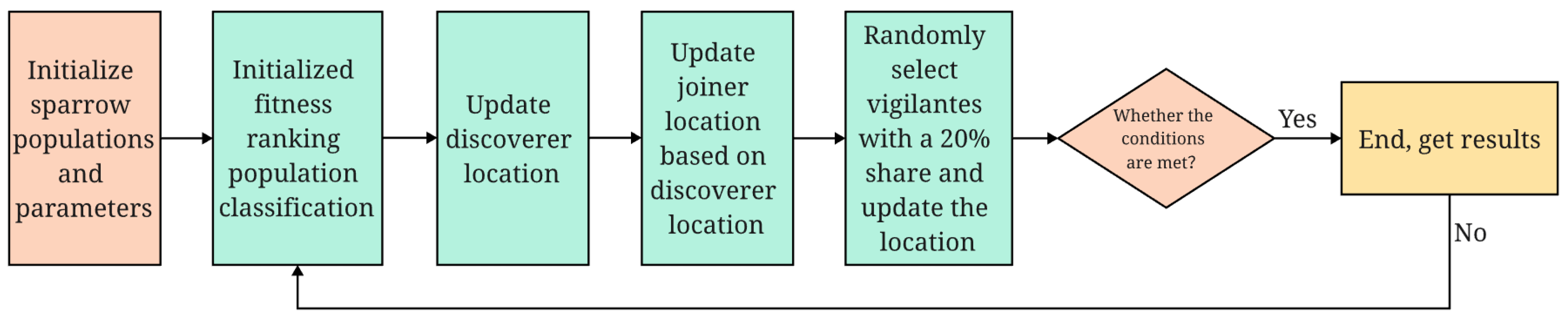
Most of the monitoring data generated during the operation of hydraulic buildings are structured time series data. The LSTM model is an improved recurrent neural network (RNN) model with special units (i.e., memory modules) added to the RNN, which is compatible with processing time series data of dams [20,21,22]. While learning the current information, the LSTM model also extracts the correlation of data with large span on the time series, so as to reduce the rate of information loss and achieve lasting memory. Its effective use in dam safety monitoring and good performance in longer time series data prediction has been verified through long-term research. As shown in Figure 1, the LSTM model structure consists of a forget gate ($f_t^l$), input gate ($i_t^l$), and output gate ($o_t^l$), and the decision to update or discard data is made through these three components. First, the forgetting gate decides with a certain probability whether to retain the state of the cell at the previous moment and selects the proportion of the information to be retained by utilizing the output ($h_t-1$) of the hidden layer from the previous time step and the input ($x_t$) at the current time step, and the two parameters are fed into the sigmoid activation function ($\sigma$) to obtain the output of the forgetting gate ($f_t$). $f_t$ and $\sigma$ are calculated as:

$$f_t=\sigma \left(W_f·\left(h_{t-1},x_i\right)+b_f\right)$$

(1)

$$\sigma \left(x\right)=1/\left(1-e^{-x}\right)$$

(2)

where $W_f$ is weight matrixes of the forget gate, $b_f$ is deviation vectors, and $\sigma$ is the logistic sigmoidal function. The input vector at time t and the output vector at time $t-1$$h_{t-1}$ are represented by $x_i$ and $h_{t-1}$, respectively. The forget gate output $f_t$ regulates the extent to which the unit information from the previous time step is forgotten, and its values are bound within the range of [0, 1]. $f_t$ = 1 means complete retention and $f_t$ = 0 complete forgetting.

The role of the input gate is to filter the input at the current moment to determine which information needs to be stored as new information in the cell state. The introduction of new information is determined by both the sigmoid layer ($\sigma$) and the tanh layer (tanh), where the sigmoid layer ($\sigma$) determines the degree of new information entry it and the tanh layer (tanh) generates the amount of new information candidates ${\tilde{a}}_t$ at needed for storage. The relevant calculation formula is:

$$i_t=\sigma \left(W_i·\left(h_{t-1},x_i\right)+b_i\right)$$

(3)

$${\tilde{a}}_t=tanh\left(W_c·\left(h_{t-1},x_i\right)+b_c\right)$$

(4)

$$tanhx=\left(1-e^{-x}\right)/\left(1+e^{-x}\right)$$

(5)

where $W_i$, $W_c$ are weight matrixes of sigmoid layer and tanh layer, respectively, and $b_i$, $b_c$ are deviation vectors of sigmoid layer and tanh layer, respectively.

The cell state is updated by combining the previous time step’s cell state and the current time step’s input information through the forgetting and input gates. The new cell status update formula is:

$$C_t=f_t{C}_{t-1}+i_t{a}_t$$

(6)

The output gate selectively extracts relevant information from the current cell state to generate a new hidden layer. The output part of the current cell state is first determined by the sigmoid function ($\sigma$), then the current cell state is processed by the tanh function (tanh), and finally a new hidden layer $h_t$ is generated. The relevant calculation formula is:

$$h_t=o_{t}tanh{C}_t$$

(7)

$$o_t=\sigma \left(W_o·\left(h_{t-1},x_i\right)+b_o\right)$$

(8)

where $W_o$ is weight matrixes of the output gate, and $b_f$ is deviation vectors.

To summarize, the current hidden layer output $h_t$ and cell state $C_t$ of the LSTM model are influenced by the previous hidden layer output $h_{t-1}$ and cell state $C_{t-1}$, as well as the current input $x_t$ at the given moment. According to several references, the LSTM model containing more than two hidden layers is constructed. This model can better train the complex nonlinear relationship between dam deformation and impact factors [4,13].

2.2. SSA Principles

The simple implementation and high search efficiency of the SSA algorithm make it one of the most promising intelligent optimization algorithms currently available [19,23]. This algorithm divides the population of sparrows into finders and joiners, with finders searching for food and providing food locations for other groups and joiners foraging by following finders. Suppose a sparrow population consists of n sparrows and the dimension of the parameter to be optimized is d. The position matrix X represents the n sparrows in a d-dimensional space and can be denoted as:

$$X=\left[\begin{array}{cccc}{x}_1^1& x_1^2& \cdots & x_1^d\\ x_2^1& x_2^2& \cdots & x_2^d\\ ⋮& ⋮& ⋮& ⋮\\ x_n^1& x_n^2& \cdots & x_n^d\end{array}\right]G_x=\left[\begin{array}{cccc}g\left(\left[x_1^1\right.\right.& x_1^2& \cdots & \left.\left.x_1^d\right]\right)\\ g\left(\left[x_2^1\right.\right.& x_2^2& \cdots & \left.\left.x_2^d\right]\right)\\ ⋮& \\ g\left(\left[x_n^1\right.\right.& x_n^2& \cdots & \left.\left.x_n^d\right]\right)\end{array}\right]$$

(9)

where n represents the number of sparrows, while d represents the dimension of the variable being optimized, x is an individual sparrow, and the value of each row in $G_x$ represents the fitness value of the individual.

The joiner needs a large predation range to find better food, so in each iteration, the joiners position is updated as:

$$X_{i,j}^{\mathrm{iter}+1}=\left\{\begin{array}{cc}\hfill X_{i,j}·exp\left(-\frac{i}{\alpha ·ite{r}_{max}}\right)\hfill & \hfill R_2<ST\hfill \\ \hfill X_{i,j}+QL\hfill & \hfill R_2\ge ST\hfill \end{array}\right.$$

(10)

where $iter$ represents the current iteration, and $ite{r}_{max}$ is a constant representing the maximum number of iterations. $X_{i,j}$ denotes the value of the jth dimension of the ith sparrow at iteration t. $\alpha$ is a random number within the range [0, 1]. $R_2$ and $ST$ denote the alarm value and safety threshold, respectively. L represents a matrix of size 1 × d, where each element is set to 1. When $R_2<ST$, the surroundings are safe and the finder searches; when $R_2\ge ST$, there is danger, and the population abandons food and flies to other safe areas.

Joiners find food by monitoring and following the most adapted finder, and when the less adapted joiner does not get food, it makes a location change to get more food. The location change formula is:

$$X_{i,j}^{iter+1}=\left\{\begin{array}{cc}Q·exp\left(\frac{X_{\mathrm{worst}}-X_{i,j}^{iter}}{i^2}\right)& i>\frac{n}{2}\\ X_p^{iter+1}+\left|X_{i,j}-X_p^{iter+1}\right|A^{+}L& \mathrm{otherwise}\end{array}\right.$$

(11)

where $X_p$ represents the best position currently occupied by the producer, while $X_{worst}$ represents the worst position. A is a matrix of size 1 ×d, where the elements are randomly assigned either 1 or −1, and $A^{+}=A^T{\left(A{A}^T\right)}^{-1}$. $i>n/2$ indicates that the i-th accession with a lower fitness value is hungry and unable to forage.

Once the proportion of sparrows capable of recognizing danger reaches 10% to 20% of the total population, their initial positions are randomly generated. Afterwards, the initialized finders and joiners engage in competition for food and update their positions until the maximum number of iterations is reached. Finally, the sparrow with the highest global fitness value is identified as the global optimal solution. The specific algorithm flow chart is shown in Figure 2. The equation for updating the position of this class of sparrows is:

$$X_{i,j}^{\mathrm{iter}+1}=\left\{\begin{array}{cc}\hfill X_{\mathrm{best}}^{\mathrm{iter}}+\beta \left|X_{i,j}^{\mathrm{iter}}-X_{\mathrm{best}}^{\mathrm{iter}}\right|\hfill & \hfill f_i<f_g\hfill \\ \hfill X_{i,j}^{\mathrm{iter}}+K\left|\frac{X_{i,j}^{\mathrm{iter}}-X_{\mathrm{worst}}^{\mathrm{iter}}}{\left(f_i-f_w\right)+\epsilon }\right|\hfill & \hfill f_i=f_g\hfill \end{array}\right.$$

(12)

where $X_{best}$ represents the current best position. The parameter $\beta$ is a step control parameter, which is a random number with a normal distribution having a mean of 0 and a variance of 1. K takes values in the range [−1, 1] as a random number. $f_g$ and $f_w$ denote the current global best and worst fitness values, respectively. Additionally, $\epsilon$ is a small constant used to prevent zero-division errors.

3. SSA–LSTM Based Dam Deformation Prediction Model

3.1. Selection of Feature Factors and Model Parameters

According to the dam engineering principle, the displacement $\delta$ generated at any point of the dam under the effect of water pressure and temperature can be divided into three components according to the cause [24,25], which are the water pressure component $\left({\delta }_H\right)$, the temperature component $\left({\delta }_T\right)$, and the aging component $\left({\delta }_{\theta }\right)$, with the formula:

$$\delta ={\delta }_H+{\delta }_T+{\delta }_{\theta }$$

(13)

Depending on the type of dam, the components of Formula (13) are slightly different, and this paper focuses on the deformation of any point on the gravity dam. According to the structural characteristics of the gravity dam and the actual condition of the project, under the effect of the upstream reservoir, the horizontal displacement on the gravity dam is linearly related to the water depth H, $H^2$, $H^3$, which can be expressed by Equation (14). The temperature at any point within the concrete of the dam can be approximated by a periodic function, assuming that the temperature displacement is linearly related to the concrete temperature, and the harmonic sine function can be chosen as a factor, i.e., the displacement caused by the temperature effect for a gravity dam can be expressed by Equation (15). The aging component of the dam reflects the creep, plastic deformation of the concrete and bedrock, as well as the compression deformation of the bedrock geological structure. During normal operation, the time-dependent displacement of the dam typically exhibits a sharp change at the beginning and gradually stabilizes towards the end. For concrete gravity dams, the aging component can be expressed by Equation (16). In summary, there are nine initial input variables to the model, namely H, $H^2$, $H^3$, $sin2\pi it/365$, $cos2\pi it/365$, $sin4\pi it/365$, $cos4\pi it/365$, $\theta$, and $ln\theta$. The specific calculation formula is:

$$\begin{array}{c}{\delta }_H=\sum _{i=1}^3{a}_i{H}^i\end{array}$$

(14)

$$\begin{array}{c}{\delta }_T=\sum _{i=1}^2\left(b_{i}sin\frac{2\pi it}{365}+c_{i}cos\frac{2\pi it}{365}\right)\end{array}$$

(15)

$$\begin{array}{c}{\delta }_{\theta }=d_1(\theta -{\theta }_0)+d_2(ln\theta -ln{\theta }_0)\end{array}$$

(16)

where H represents the upstream reservoir level; $a_i$, $b_i$, $c_i$, $d_1$, and $d_2$ represent the corresponding linear coefficients; t is the number of days from the initial date of dam observation to the current observation date; $t_0$ is the number of days from the initial date of the dam observation to the initial date of the modeling; $\theta$ is $t/100$; and ${\theta }_0$ is $t_0/100$.

In LSTM networks, parameters such as training rate, number of training epochs (Epoch), batch size, number of neurons in the first layer1 (units1) and number of neurons in the first layer2 (units2) are the key indicators affecting the prediction accuracy, and these parameters directly determine the network structure of the LSTM model. Therefore, the SSA optimization algorithm is used to automatically optimize the five parameters of the LSTM model. The training rate refers to the step size of the parameter update in each iteration of the model. The size of the training rate affects the convergence speed and stability of the model, usually by back propagation, which calculates the gradient of each parameter against the loss function and then updates the model parameters based on the gradient and the training rate. The number of training epochs is the number of iterations of the model over the entire training dataset. The size of the training epochs affects the model’s ability to fit and generalize. In each iteration, the model performs a forward and backward propagation using all the samples in the training dataset and then updates the model parameters. Batch size is the number of samples processed simultaneously in a training session. The size of the batch size also affects the training speed and performance of the model, and it is usually appropriate to adjust the size of the batch size depending on the test. The number of neurons is usually determined by the complexity of the model and the complexity of the task, so it also needs to be sized depending on the different tests.

3.2. Prediction Accuracy Evaluation Index

To assess the accuracy of the predictions, this model employs three evaluation metrics: mean absolute error (MAE), mean absolute percentage error (MAPE), and root mean square error (RMSE). These metrics are used comprehensively to provide a comprehensive assessment of the model’s performance. The specific calculation formula is shown in Equations (17)–(19).

$$\begin{array}{c}MAE\left(y_i,\widehat{y}\right)=\frac{1}{m}\sum _1^m\left|y_{i-}\widehat{y}\right|\hfill \end{array}$$

(17)

$$\begin{array}{c}MAPE\left(y_i,\widehat{y}\right)=\frac{1}{m}\sum _1^m\frac{\left|y_{i-}\widehat{y}\right|}{\left|y_i\right|}\hfill \end{array}$$

(18)

$$\begin{array}{c}RMSE\left(y_i,\widehat{y}\right)=\sqrt{\frac{1}{m}{\sum }_1^m{\left(y_{i-}\widehat{y}\right)}^2}\hfill \end{array}$$

(19)

where $\widehat{y}$ represents the predicted value of the i-th sample, $y_i$ represents the corresponding true value, and m represents the total number of data to be predicted.

MAE reflects the actual situation of prediction error, MAPE evaluates the model accuracy, and RMSE is used to evaluate the prediction accuracy. For example, smaller values of the three parameters indicate higher accuracy of the prediction model and a better prediction effect.

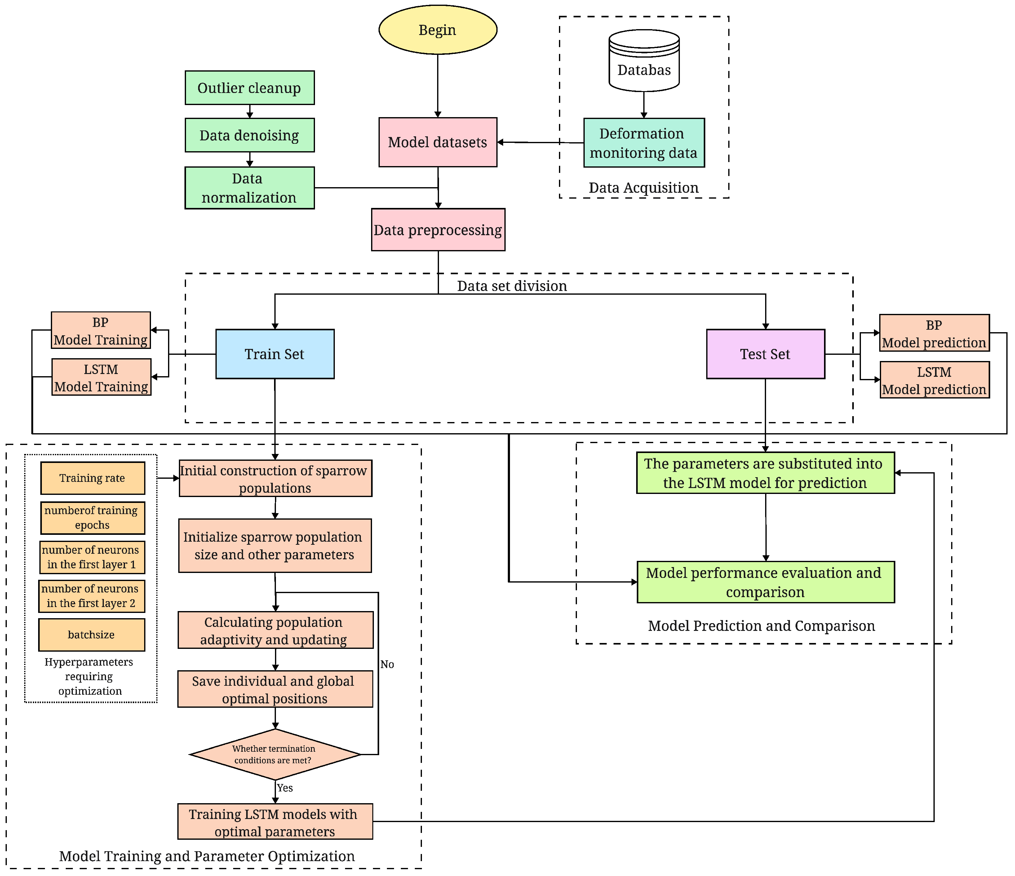
3.3. Implementation Framework

The SSA algorithm is used to determine the hyperparameters of the LSTM model, after which the optimized hyperparameters are used for model training and prediction by means of parameter transfer to optimize the performance of the model. This combination can improve the prediction accuracy and stability and effectively handle the complex temporal relationships in dam monitoring data. The implementation framework of the SSA–LSTM-based dam deformation prediction model proposed in this paper is shown in Figure 3. The specific process is as follows:

(1)

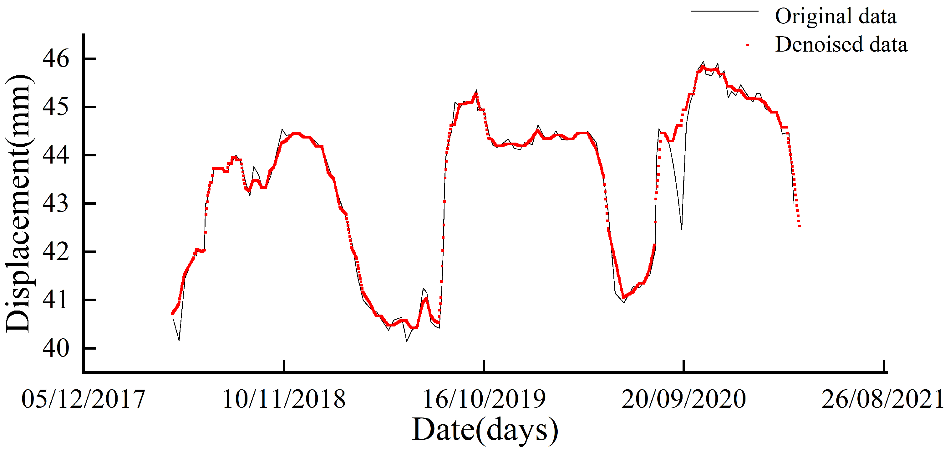
Data preprocessing. To improve the predictive capability of the dam monitoring model, it is necessary to clean and transform the prototype observation data in advance. The first step is to clean up outliers and attempt to eliminate or reduce noise interference in the data. If the cleaning effect does not meet the requirements, various data denoising methods can be tested by considering the data structure. It may even be necessary to combine multiple denoising methods to achieve the desired cleaning effect. Commonly used data denoising methods include mean filtering, Gaussian filtering, and wavelet denoising. The Symlet wavelet filtering denoising method is based on the principle of wavelet analysis and threshold processing. It involves wavelet decomposition and reconstruction of data to achieve noise removal. Gaussian filtering, on the other hand, uses the shape of a Gaussian function to smooth the data and reduce the effect of noise through weighted averaging of the neighborhood around each data point. After clearing outliers, any missing parts of the data can be interpolated. Additionally, normalizing the data is necessary to standardize the baseline values and dispersion of different features in the sample matrix. By following these preprocessing steps, a more accurate and reliable database can be provided for the dam monitoring model.

(2)

Parameter optimization. Using the four equations mentioned in Section 2.2, the discoverer, joiner, and vigilant positions are updated in the iterations, and the fitness values are calculated. At the end of the final iteration, the global optimal sparrow position is output, and the optimal parameters of the LSTM model are obtained.

(3)

Model training and prediction. The training and prediction datasets are used to train and predict the LSTM model, with hyperparameters determined by SSA. The accuracy of the model’s predictions is assessed by comparison with the true values from the test set. Additionally, the optimal hyperparameters are applied to different models for visual comparison to further evaluate the model’s performance. Detailed descriptions of each model’s prediction, along with model evaluation metrics, are considered to identify the optimal model.

4. Case Study

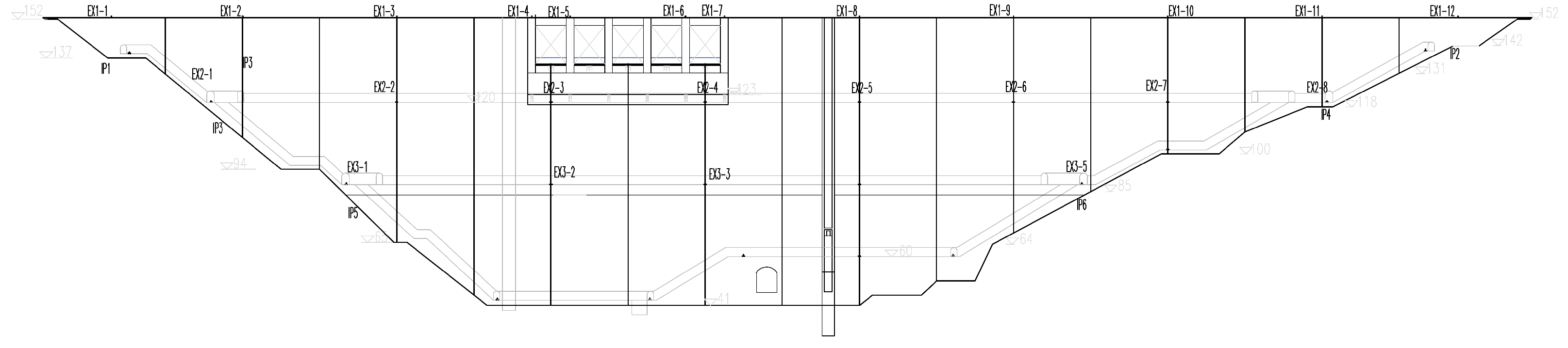
4.1. Project Overview

The object of this study is a 112 m high crushed concrete gravity dam with a crest elevation of 153.00 m, a crest width of 6 m, and a total installed capacity of 193.2 MW. The reservoir has a certified flood level of 151.88 m, a normal storage level of 150.00 m, and a dead water level of 130.00 m. It has a total storage capacity of 717.3 million m${}^3$ and consists of 10 dam sections. The main project started in September 2007 and was completed in November 2011. The dam is equipped with tension lines for monitoring downstream deformation at elevations of 153 m, 120 m, and 88 m in the corridor. Additionally, eight inverted plumb line measurement points were installed at elevations of 153 m, 120 m, 88 m, 60 m, and 43 m on both the left and right banks of the dam. Tie lines were placed in the corridor at 153 m, 120 m, and 88 m for monitoring downstream deformation as well. The tie line measurement points were numbered EX3-1a to EX3-5a in the corridor at 88 m and EX2-1a to EX2-8a in the corridor at 120 m, as shown in Figure 4. Based on preliminary observation of the monitoring data, it was noted that most of the instruments exhibited larger displacements in the downstream direction. Therefore, the training and prediction of the monitoring model focused mainly on downstream displacement deformation. For this study, data from 5 May 2018 to 6 January 2022 were selected. Four measurement points, namely EX3-4a, EX3-3a, EX2-7a, and EX2-6a, were chosen, each with approximately 180 actual raw data points. Data were measured approximately four times per month. The training set comprised the first 80% of the data, while the remaining 20% was used as the test set. The water level change process line during the selected time period and the actual measured deformation change process line of the EX3-4 measurement point are presented in Figure 5.

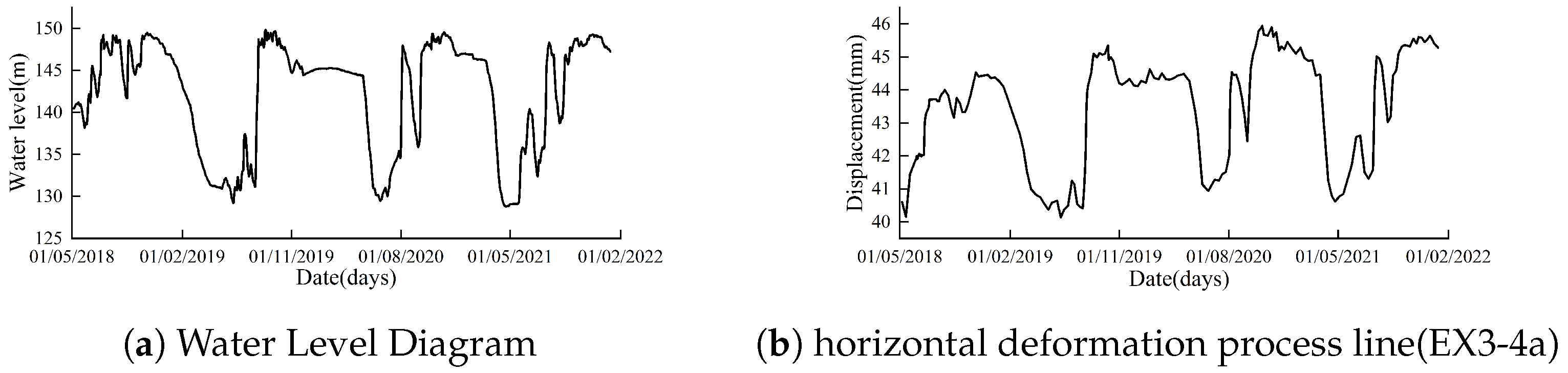
4.2. Data Preprocessing Results

The deformation data of the four measurement points fluctuate greatly during the selected time period, and there are some particularly obvious outliers, which are not obvious with the use of a single denoising algorithm. Since each denoising algorithm has its unique advantages and applicability range, two algorithms, Gaussian filtering and Symlet wavelet filtering, were selected for overlapping denoising of the original data through the comparison of multiple denoising algorithms in order to better reflect the nature and characteristics of the monitoring data, which complement each other in terms of data characteristics and noise types and obtain obvious denoising effects. Afterwards, the missing data were interpolated using the “interpolate” linear function to further improve the quality and accuracy of the data. The results of preprocessing the data of EX3-4 measurement points training part were compared with the original data curve as shown in Figure 6. While denoising, the data were finally normalized in order to improve the convergence rate of the algorithm.

4.3. SSA Algorithm Optimization Search Results

In this study, five parameters, namely training rate, number of training epochs (Epoch), number of neurons in the first layer (units1), number of neurons in the second layer (units2), and batch size, were used as hyperparameters for the optimization search. Combined with the model framework established in the previous paper, the SSA algorithm was initialized, while several experiments and optimization searches were conducted in the range of parameter values. After several observations and experiments, the five parameters were defined as [0.001, 0.01], [50, 200], [1, 80], [20, 200], and [20, 200], and the sparrow population size was set to 20, of which 10% were alerters and 20% were finders, with an alert threshold of 0.8 and 10 iterations. Due to the inconsistent data characteristics and data structure of each measurement point, and even the different intrinsic components of the data, the LSTM parameters are different in the optimization search. The results of the LSTM model parameter ranges obtained after multiple search for the four measurement points are shown in

Table 1. Hyperparameter optimization results.

Parameters	Range	Averaging
Training rate (lr)	0.001	0.001
Number of training epochs (Epoch)	100–112	106
Number of neurons in the first layer (units1)	104–130	169
Number of neurons in the first layer (units2)	244–256	250
batch_size	12–18	15

. Furthermore, considering the overall prediction effect of the model, the result of the search was averaged by running the search process several times. The analysis and comparison of the prediction effects of the averaged model found that it met the prediction requirements of most measurement points and could obtain better prediction results, which ensured the stability and reliability of the model. Therefore, the averaging of the search parameters with a comprehensive optimization strategy is able to obtain reliable search parameters. In this study, the model parameters obtained after averaging were applied in the later prediction analysis. The results of the averaging of the taken parameters are shown in Table 1.

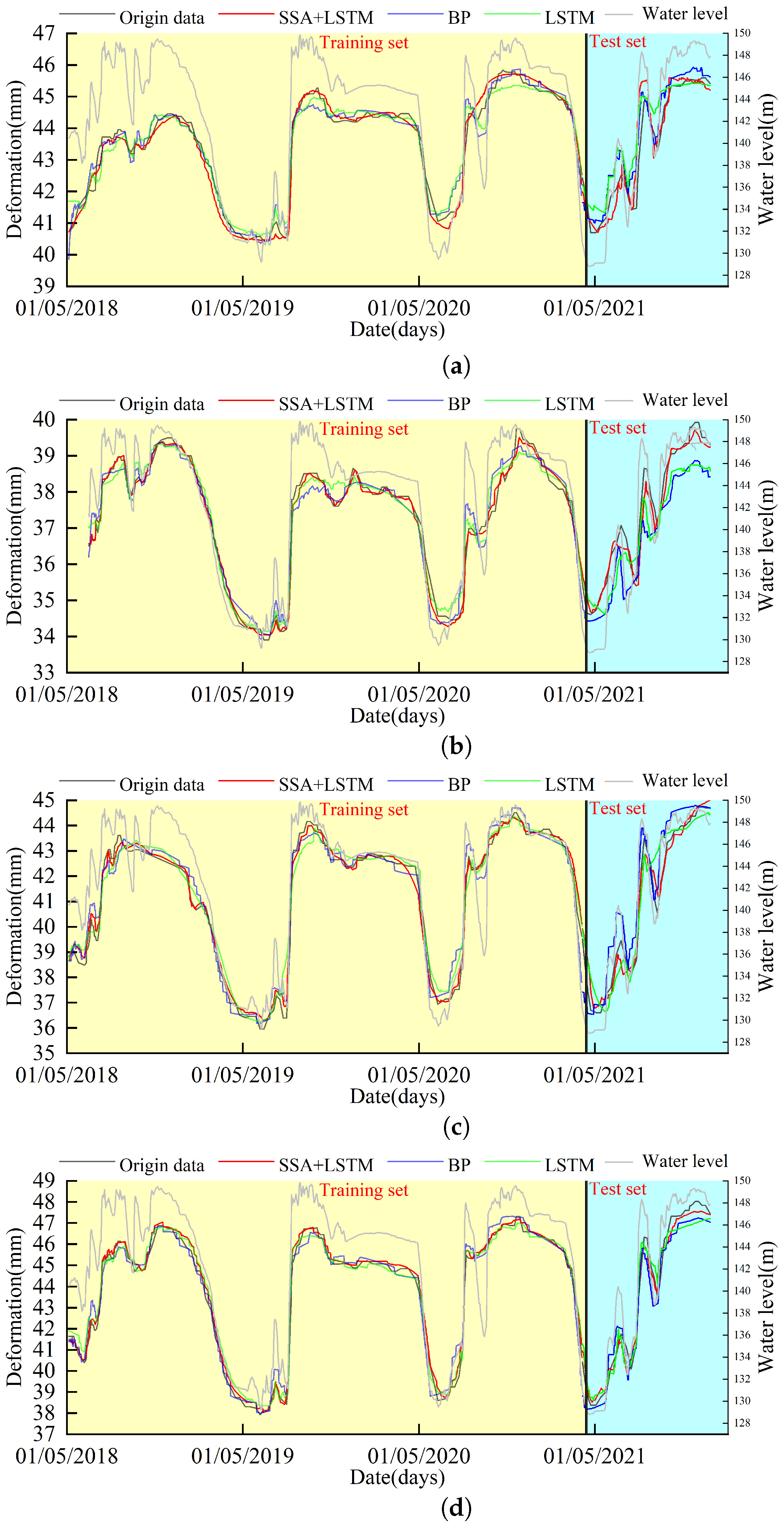
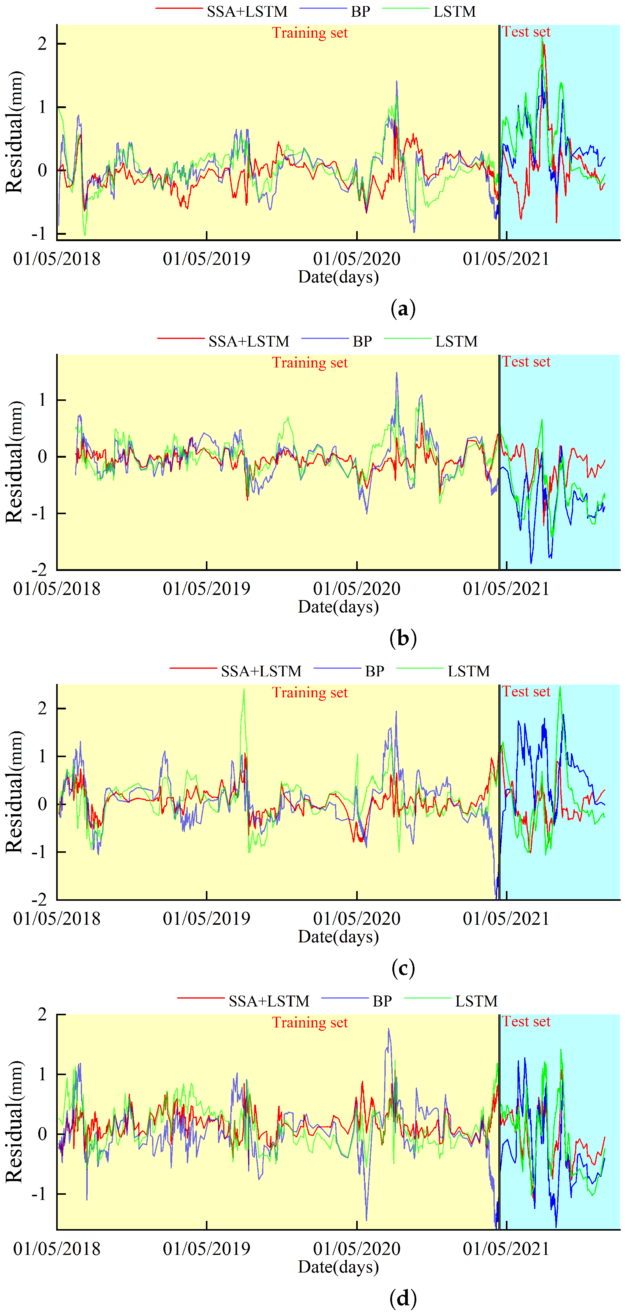
4.4. Contrast Analysis

The LSTM model was retrained, and predictions were made after its optimization using the SSA algorithm to obtain the averaged optimal parameters. For comparison, the default LSTM model was initially set with 100 neurons in the first layer1, 200 neurons in the second layer2, 20 training epochs, a batch size of 10, and a learning rate of 0.005. The non-optimized LSTM model may suffer from issues such as gradient vanishing or exploding, but through multiple tests, basic hyperparameters were determined, allowing for a visual comparison of the optimized and non-optimized model’s predictions. Additionally, to provide further comparability, an arbitrary neural network model was selected with 10 neurons in the first layer1, 20 neurons in the second layer2, a maximum iteration of 300, a batch size of 20, and a learning rate of 0.005, and it was compared with the optimized LSTM model and the non-optimized LSTM model. Although the BP model’s sensitivity to time series data may not be ideal, it is one of the most common classical neural network models, and comparing it with the optimized model can further demonstrate the performance improvements. The three models were trained and tested on four selected data points, and all three models use the same “Adam” optimizer.

Table 2. Comparison of performance indicators of different measurement points.

Monitoring Point	Model	MAE (mm)	RMSE (mm)	MAPE (%)
EX3-4a	LSTM-SSA	5 × 10${}^{-5}$	0.027	0.152
	BP	6.5 × 10${}^{-4}$	0.233	0.939
	LSTM	7.3 × 10${}^{-4}$	0.932	2.130
EX3-3a	LSTM-SSA	4.1 × 10${}^{-5}$	0.05	0.402
	BP	2.4 × 10${}^{-4}$	0.11	1.791
	LSTM	4.0 × 10${}^{-4}$	0.496	1.173
EX2-7a	LSTM-SSA	1.3 × 10${}^{-4}$	0.207	0.097
	BP	1.3 × 10${}^{-4}$	0.196	0.278
	LSTM	1.4 × 10${}^{-4}$	0.011	0.670
EX2-6a	LSTM-SSA	1.2 × 10${}^{-4}$	0.191	0.376
	BP	1.7 × 10${}^{-4}$	0.247	0.481
	LSTM	1.9 × 10${}^{-4}$	0.250	0.502

presents a comparative performance analysis of the models based on various performance metrics. It is evident that the SSA–LSTM model outperforms the LSTM and BP models, as indicated by the decreased EMAE, RMSE, and MAPE values. The MAPE of the SSA–LSTM model ranges from 0.097% to 0.402%, while the MAPE of the BP model ranges from 0.278% to 1.791%. By comparing these values, the error reduction in prediction accuracy ranges from 0.181% to 1.389% when comparing with the BP model and from 0.405% to 1.728% when comparing with the LSTM model. Specifically, for the best overall fitting data point, EX3-4a, the SSA–LSTM model shows an improvement of 0.787% in MAPE compared to the BP model and an improvement of 1.978% compared to the LSTM model, demonstrating a better predictive performance. Furthermore, the MAE of the EX3-4a data point is reduced by 6 × 10${}^{-3}$ mm and 6.8 × 10${}^{-3}$ mm when compared to the other two models, effectively reducing prediction errors. The RMSE of the EX3-4a data point is reduced by 0.206 mm and 0.905 mm when compared to the other two models, indicating significant improvements in prediction accuracy by the proposed SSA–LSTM model, with all performance indicators surpassing the other two models. The comparative analysis of the three metrics shows that the overall model performance is stable without significant deviations. It can be concluded that the SSA-optimized LSTM model enhances the model’s global optimization capability, resulting in more reliable prediction results.

To further verify the model accuracy, the training and prediction results were demonstrated for four measurement points using three models. Figure 7 shows the fitting results of the training and prediction models, and Figure 8 shows the residuals. The SSA–LSTM model fits better than the other models, the horizontal displacement residuals are significantly smaller than the other models, and the SSA–LSTM model almost completely overlaps with the real curve in the prediction curve of EX3-4a measurement points, effectively predicting the complex nonlinear variation trend between the dam deformation and impact factors in the short term. The SSA–LSTM model is almost completely consistent with the real curve, which effectively predicts the complex nonlinear variation trend between dam deformation and impact factors in the short term and accurately grasps the variation pattern, further illustrating the high efficiency of the model prediction performance of the SSA algorithm for optimization. This validation shows that the dam monitoring data analysis based on the artificial intelligence algorithm has a good prediction effect and can be used in the later work of dam monitoring data analysis.

5. Conclusions

In this study, three models, namely SSA–LSTM, BP, and LSTM, were used to construct a deformation prediction model for four measurement points of a concrete gravity dam, and the following conclusions were drawn by comparing and analyzing the prediction and residual effects:

(1)

For the random outliers in the dam deformation monitoring data, multiple denoising algorithm weights are used to complement each other in terms of data characteristics and noise types, which can obtain a better denoising effect on the measured data and obtain real data that can reflect the working state of the dam, effectively eliminating the influence of coarse differences on the prediction accuracy of the model.

(2)

Due to the different characteristics and intrinsic components of each measurement point, the SSA optimization algorithm proposed the optimal range of parameters and averaged parameter values, which can better obtain the characteristics of the dam deformation sequence in time sequence and take into account the backward and forward correlation of the input information, thus improving the prediction accuracy of the LSTM model.

(3)

The SSA–LSTM model established in this paper has higher prediction accuracy and stability than the BP and LSTM models, and the modeling results are consistent with the actual engineering situation, providing a new technique for predicting dam deformation with high accuracy. The method is simple and efficient and can be applied to the prediction analysis of other monitoring effects of dams with modification.

In the later stage, further improvements can be made to the optimization strategies and solving methods of the SSA optimization algorithm itself to enhance the extraction of features and temporal correlations in dam deformation sequences. Additionally, the LSTM model can be combined with other neural network models to improve overall predictive performance. Depending on the data structure and specific problem, leveraging the strengths of different models can effectively address challenges in practical applications.

References

1. Lin, C.; Wang, X.; Su, Y.; Zhang, T.; Lin, C. Deformation Forecasting of Pulp-Masonry Arch Dams via a Hybrid Model Based on CEEMDAN Considering the Lag of Influencing Factors. J. Struct. Eng. 2022, 148, 04022078. [Google Scholar] [CrossRef]
2. Wang, S.; Yang, B.; Chen, H.; Fang, W.; Yu, T. LSTM-Based Deformation Prediction Model of the Embankment Dam of the Danjiangkou Hydropower Station. Water 2022, 14, 2464. [Google Scholar] [CrossRef]
3. Lin, C.; Weng, K.; Lin, Y.; Zhang, T.; He, Q.; Su, Y. Time Series Prediction of Dam Deformation Using a Hybrid STL-CNN-GRU Model Based on Sparrow Search Algorithm Optimization. Appl. Sci. 2022, 12, 11951. [Google Scholar] [CrossRef]
4. Qu, X.; Yang, J.; Chang, M. A Deep Learning Model for Concrete Dam Deformation Prediction Based on RS-LSTM. J. Sens. 2019, 2019, 4581672. [Google Scholar] [CrossRef]
5. Bui, K.T.T.; Torres, J.F.; Gutierrez-Aviles, D.; Nhu, V.H.; Bui, D.T.; Martinez-Alvarez, F. Deformation forecasting of a hydropower dam by hybridizing a long short-term memory deep learning network with the coronavirus optimization algorithm. Comput.-Aided Civ. Infrastruct. Eng. 2022, 37, 1368–1386. [Google Scholar] [CrossRef]
6. Li, M.; Li, M.; Ren, Q.; Li, H.; Song, L. DRLSTM: A dual-stage deep learning approach driven by raw monitoring data for dam displacement prediction. Adv. Eng. Inform. 2022, 51, 101510. [Google Scholar] [CrossRef]
7. Yang, S.; Han, X.; Kuang, C.; Fang, W.; Zhang, J.; Yu, T. Comparative Study on Deformation Prediction Models of Wuqiangxi Concrete Gravity Dam Based on Monitoring Data. CMES—Comput. Model. Eng. Sci. 2022, 131, 49–72. [Google Scholar] [CrossRef]
8. Vapnik, V.; Vashist, A. A new learning paradigm: Learning using privileged information. Neural Netw. 2009, 22, 544–557. [Google Scholar] [CrossRef]
9. Su, H.; Chen, Z.; Wen, Z. Performance improvement method of support vector machine-based model monitoring dam safety. Struct. Control Health Monit. 2016, 23, 252–266. [Google Scholar] [CrossRef]
10. Zhu, S.; Wu, S. Application of Gaussian process regression models in river water temperature modelling. J. Huazhong Univ. Sci. Technol. Nat. Sci. 2019, 46, 122–126. [Google Scholar]
11. Hochreiter, S.; Schmidhuber, J. Long short-term memory. Neural Comput. 1997, 9, 1735–1780. [Google Scholar] [CrossRef] [PubMed]
12. Dai, B.; Chen, B. Chaos-based dam monitoring sequence wavelet RBF neural network prediction model. Water Resour. Hydropower Eng. 2016, 47, 80–85. [Google Scholar]
13. Liu, W.; Pan, J.; Ren, Y.; Wu, Z.; Wang, J. Coupling prediction model for long-term displacements of arch dams based on long short-term memory network. Struct. Control Health Monit. 2020, 27, e2548. [Google Scholar] [CrossRef]
14. Li, X.; Zhou, H.; Su, R.; Kang, J.; Sun, Y.; Yuan, Y.; Han, Y.; Chen, X.; Xie, P.; Wang, Y.; et al. A mild cognitive impairment diagnostic model based on IAAFT and BiLSTM. Biomed. Signal Process. Control 2023, 80, 104349. [Google Scholar] [CrossRef]
15. Manna, T.; Anitha, A. Precipitation prediction by integrating Rough Set on Fuzzy Approximation Space with Deep Learning techniques. Appl. Soft Comput. 2023, 139, 110253. [Google Scholar] [CrossRef]
16. Tang, Y.; Chen, Z.; Huang, Z.; Nong, Y.; Li, L. Visual Measurement of dam concrete cracks based on U-net and improved thinning algorithm. J. Exp. Mech. 2022, 37, 209–220. [Google Scholar]
17. Xue, J.; Shen, B. A novel swarm intelligence optimization approach: Sparrow search algorithm. Syst. Sci. Control Eng. 2020, 8, 22–34. [Google Scholar] [CrossRef]
18. Hinchey, M.G.; Sterritt, R.; Rouff, C. Swarms and swarm intelligence. Computer 2007, 40, 111–113. [Google Scholar] [CrossRef]
19. Bonabeau, E.; Meyer, C. Swarm intelligence. A whole new way to think about business. Harv. Bus. Rev. 2001, 79, 106–114. [Google Scholar] [PubMed]
20. Sherstinsky, A. Fundamentals of Recurrent Neural Network (RNN) and Long Short-Term Memory (LSTM) network. Phys. D-Nonlinear Phenom. 2020, 404, 132306. [Google Scholar] [CrossRef] [Green Version]
21. Greff, K.; Srivastava, R.K.; Koutnik, J.; Steunebrink, B.R.; Schmidhuber, J. LSTM: A Search Space Odyssey. IEEE Trans. Neural Netw. Learn. Syst. 2017, 28, 2222–2232. [Google Scholar] [CrossRef] [PubMed] [Green Version]
22. Yang, H.; Yue, J.; Xing, Y.; Zhou, Q. Research on Dam Deformation Prediction Based on Deep Fully Connected Neural Network. J. Geod. Geodyn. 2021, 41, 162–166. [Google Scholar]
23. Liu, X.; Guo, H. Air quality indicators and AQI prediction coupling long-short term memory (LSTM) and sparrow search algorithm (SSA): A case study of Shanghai. Atmos. Pollut. Res. 2022, 13, 101551. [Google Scholar] [CrossRef]
24. Wu, Z.R.; Gu, C.S.; Su, H.Z.; Chen, B. Review and prospect of calculation analysis methods in hydro-structure engineering. J. Hohai Univ. Nat. Sci. 2015, 43, 395–405. [Google Scholar]
25. Yang, D.; Gu, C.; Zhu, Y.; Dai, B.; Zhang, K.; Zhang, Z.; Li, B. A Concrete Dam Deformation Prediction Method Based on LSTM with Attention Mechanism. IEEE Access 2020, 8, 185177–185186. [Google Scholar] [CrossRef]
Figure 1. Structure diagram of LSTM.
Applsci 13 07375 g001
Figure 2. SSA algorithm flowchart.
Applsci 13 07375 g002
Figure 3. SSA–LSTM model prediction process.
Applsci 13 07375 g003
Figure 4. Dam deformation monitoring point layout program.
Applsci 13 07375 g004
Figure 5. Reservoir water level and horizontal deformation process line.
Applsci 13 07375 g005
Figure 6. Denoising comparison chart.
Applsci 13 07375 g006
Figure 7. Training and prediction results chart of different model. (a) EX3-4a. (b) EX3-3a. (c) EX2-7a. (d) EX2-6a.
Applsci 13 07375 g007
Figure 8. Residual plots of different model. (a) EX3-4a. (b) EX3-3a. (c) EX2-7a. (d) EX2-6a.
Applsci 13 07375 g008