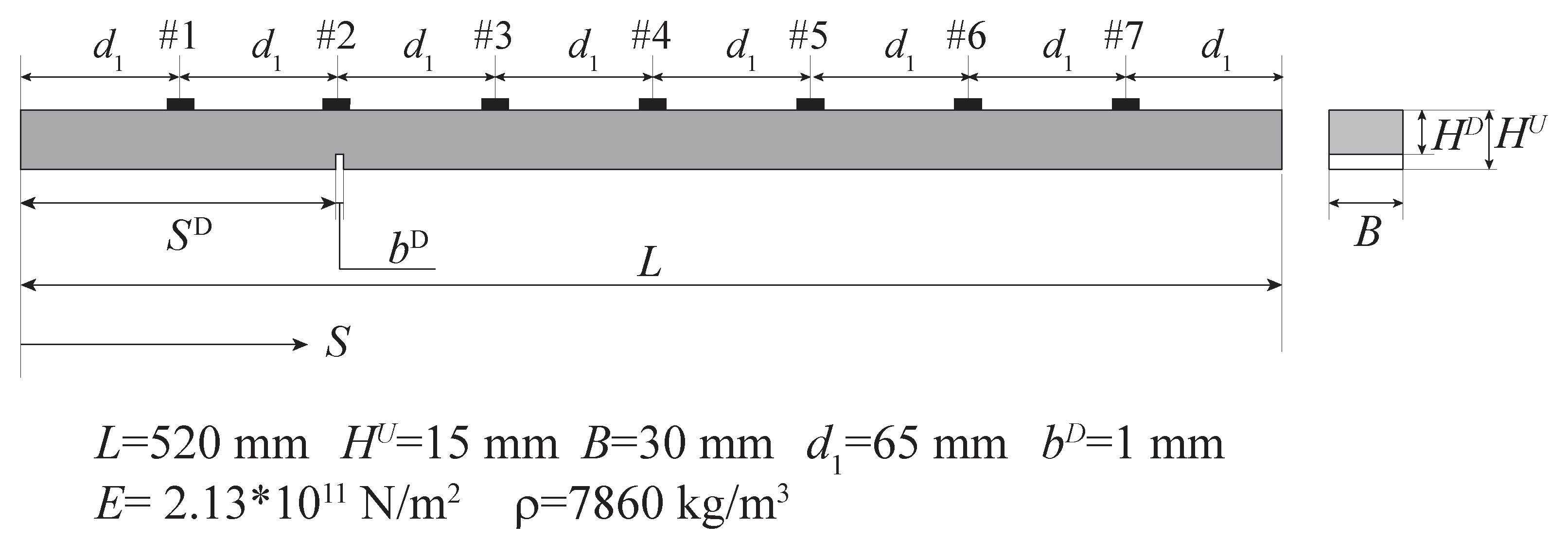
Figure 1.
Schematic representation of the beam longitudinal view (left) and of its cross section (right).
Figure 1.
Schematic representation of the beam longitudinal view (left) and of its cross section (right).
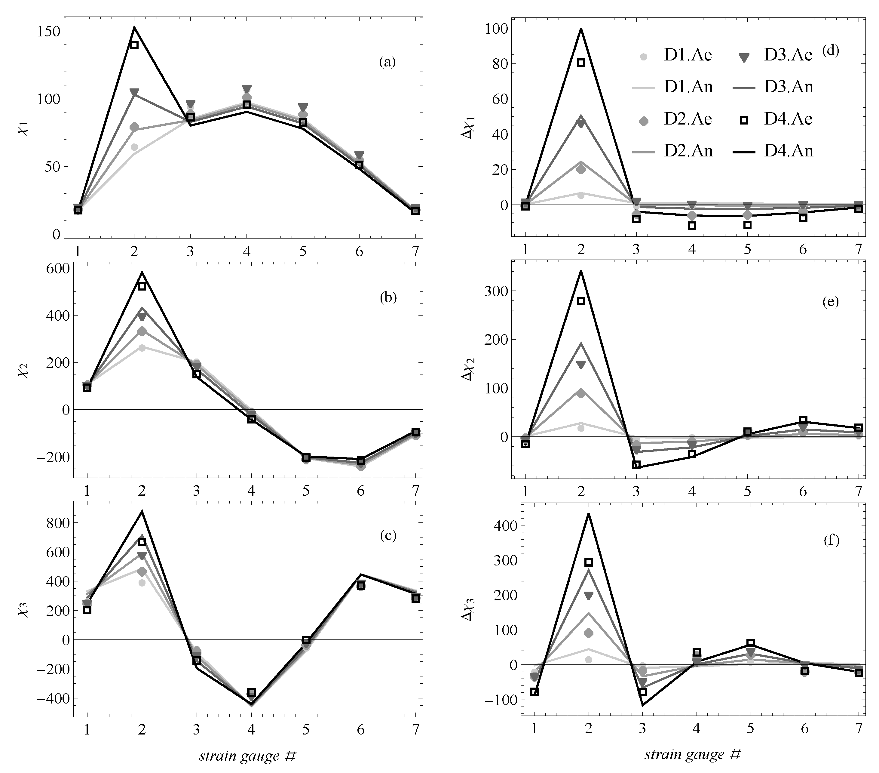
Figure 2.
Variation of modal displacements (a–c) and modal curvatures (d–f) in the four damage scenarios of location A, for the first (a,d), second (b,e) and third (c,f) mode.
Figure 2.
Variation of modal displacements (a–c) and modal curvatures (d–f) in the four damage scenarios of location A, for the first (a,d), second (b,e) and third (c,f) mode.
Figure 3.
Schematic representation of the experimental setup (a) and image of the beam in laboratory conditions (b).
Figure 3.
Schematic representation of the experimental setup (a) and image of the beam in laboratory conditions (b).
Figure 4.
Case A: experimental (e) and numerical (n) modal curvatures (first (a), second (b) and third (c) mode) and their variations due to damage (first (d), second (e) and third (f) mode).
Figure 4.
Case A: experimental (e) and numerical (n) modal curvatures (first (a), second (b) and third (c) mode) and their variations due to damage (first (d), second (e) and third (f) mode).
Figure 5.
Case B: experimental (e) and numerical (n) modal curvatures (first (a), second (b) and third (c) mode) and their variations (first (d), second (e) and third (f) mode) due to damage.
Figure 5.
Case B: experimental (e) and numerical (n) modal curvatures (first (a), second (b) and third (c) mode) and their variations (first (d), second (e) and third (f) mode) due to damage.
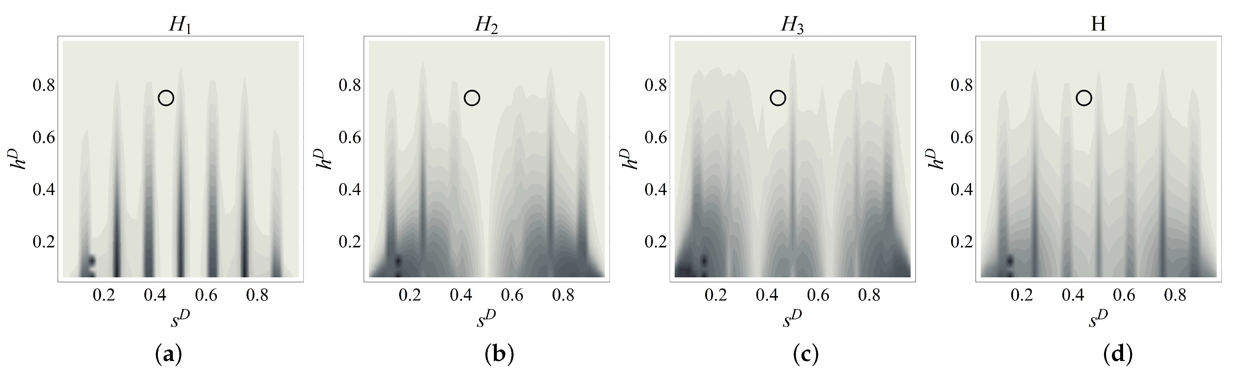
Figure 6.
Contour plots of the objective function including one ((a) i = 1, (b) i = 2, (c) i = 3) and three numerical modal curvatures ((d) i = 1, 2, 3) (coordinates of the circle are and for D2.A).
Figure 6.
Contour plots of the objective function including one ((a) i = 1, (b) i = 2, (c) i = 3) and three numerical modal curvatures ((d) i = 1, 2, 3) (coordinates of the circle are and for D2.A).
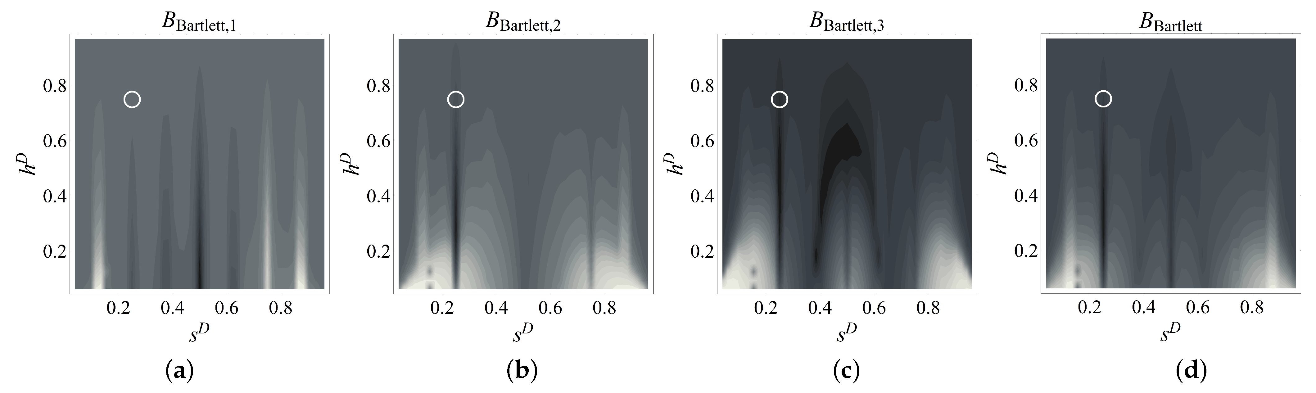
Figure 7.
Contour plots of the Bartlett beamformer including one ((a) i = 1, (b) i = 2, (c) i = 3) and three numerical modal curvatures ((d) i = 1, 2, 3) (coordinates of the circle are and for D2.A).
Figure 7.
Contour plots of the Bartlett beamformer including one ((a) i = 1, (b) i = 2, (c) i = 3) and three numerical modal curvatures ((d) i = 1, 2, 3) (coordinates of the circle are and for D2.A).
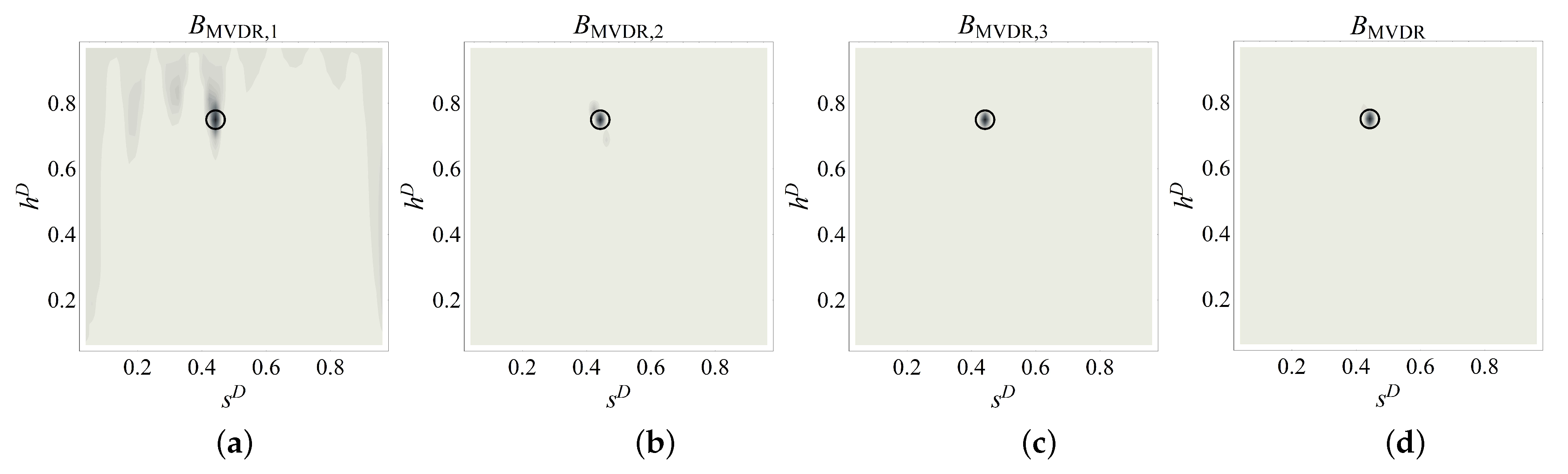
Figure 8.
Contour plots of the MVDR beamformer including one ((a) i = 1, (b) i = 2, (c) i = 3) and three numerical modal curvatures ((d) i = 1, 2, 3) (coordinates of the circle are and for D2.A).
Figure 8.
Contour plots of the MVDR beamformer including one ((a) i = 1, (b) i = 2, (c) i = 3) and three numerical modal curvatures ((d) i = 1, 2, 3) (coordinates of the circle are and for D2.A).
Figure 9.
Contour plots of the objective function including one ((a) i = 1, (b) i = 2, (c) i = 3) and three numerical modal curvatures ((d) i = 1, 2, 3) (Circle: Correct damage parameters).
Figure 9.
Contour plots of the objective function including one ((a) i = 1, (b) i = 2, (c) i = 3) and three numerical modal curvatures ((d) i = 1, 2, 3) (Circle: Correct damage parameters).
Figure 10.
Contour plots of the Bartlett beamformer including one ((a) i = 1, (b) i = 2, (c) i = 3) and three numerical modal curvatures ((d) i = 1, 2, 3) (circle: correct damage parameters).
Figure 10.
Contour plots of the Bartlett beamformer including one ((a) i = 1, (b) i = 2, (c) i = 3) and three numerical modal curvatures ((d) i = 1, 2, 3) (circle: correct damage parameters).
Figure 11.
Contour plots of the MVDR beamformer including one ((a) i = 1, (b) i = 2, (c) i = 3) and three numerical modal curvatures ((d) i = 1, 2, 3) (circle: correct damage parameters).
Figure 11.
Contour plots of the MVDR beamformer including one ((a) i = 1, (b) i = 2, (c) i = 3) and three numerical modal curvatures ((d) i = 1, 2, 3) (circle: correct damage parameters).
Figure 12.
Contour plots of the estimators for damage scenario D1.A ((a) objective function, (b) Bartlett, (c) MVDR) (circle: correct damage parameters; cross: identified parameters).
Figure 12.
Contour plots of the estimators for damage scenario D1.A ((a) objective function, (b) Bartlett, (c) MVDR) (circle: correct damage parameters; cross: identified parameters).
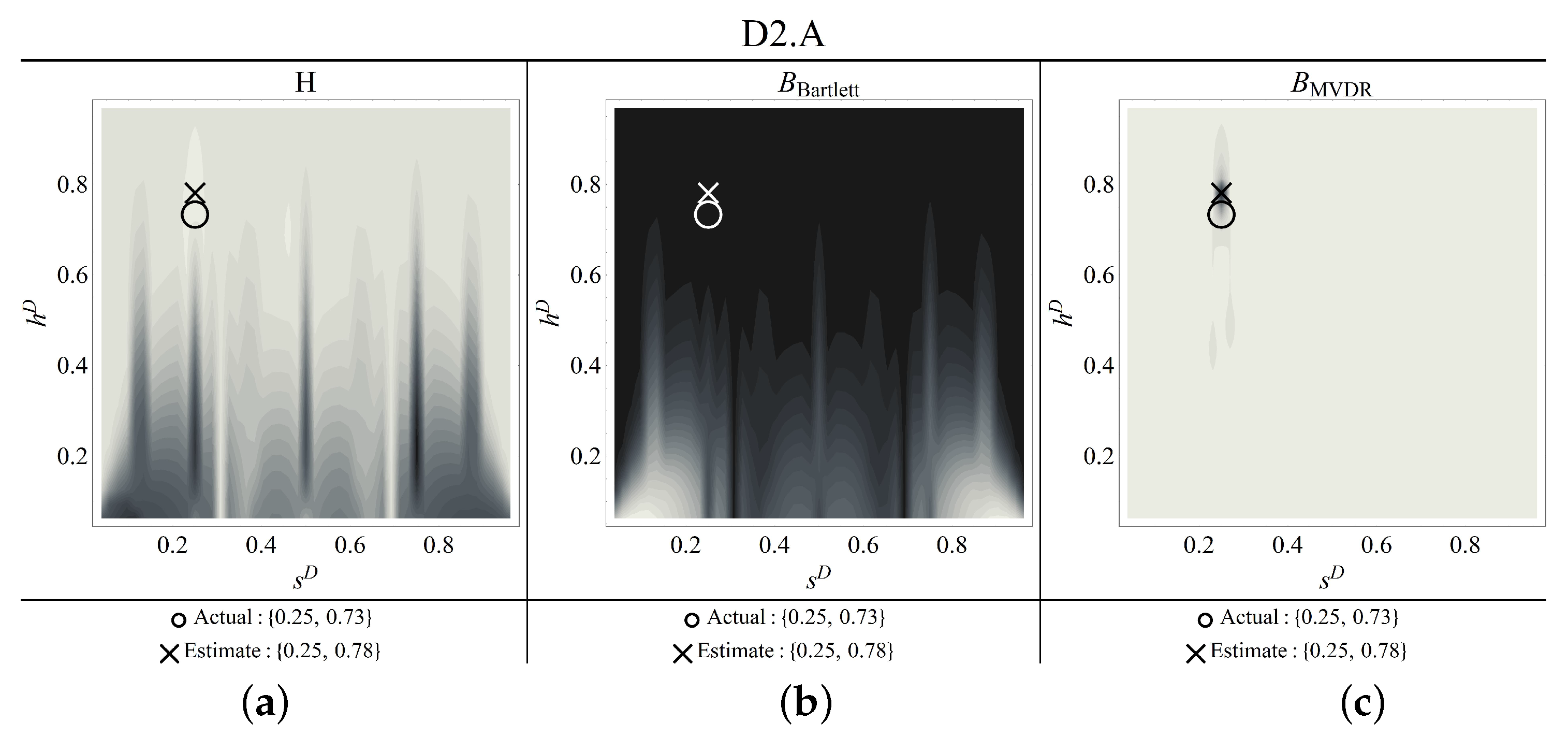
Figure 13.
Contour plots of the estimators for damage scenario D2.A ((a) objective function, (b) Bartlett, (c) MVDR) (circle: correct damage parameters; cross: identified parameters).
Figure 13.
Contour plots of the estimators for damage scenario D2.A ((a) objective function, (b) Bartlett, (c) MVDR) (circle: correct damage parameters; cross: identified parameters).
Figure 14.
Contour plots of the estimators for damage scenario D3.A ((a) objective function, (b) Bartlett, (c) MVDR) (circle: correct damage parameters; cross: identified parameters).
Figure 14.
Contour plots of the estimators for damage scenario D3.A ((a) objective function, (b) Bartlett, (c) MVDR) (circle: correct damage parameters; cross: identified parameters).
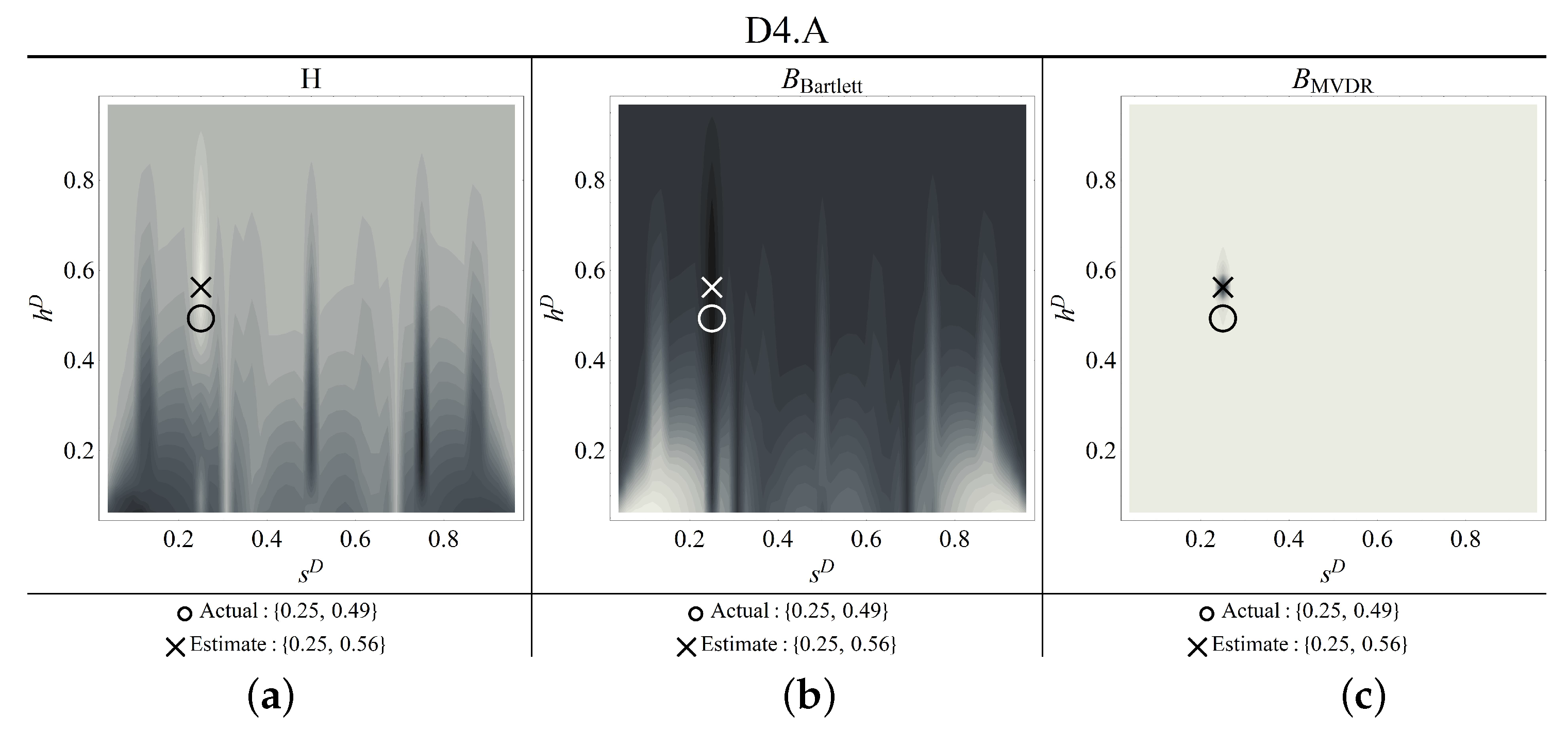
Figure 15.
Contour plots of the estimators for damage scenario D4.A ((a) objective function, (b) Bartlett, (c) MVDR) (circle: correct damage parameters; cross: identified parameters).
Figure 15.
Contour plots of the estimators for damage scenario D4.A ((a) objective function, (b) Bartlett, (c) MVDR) (circle: correct damage parameters; cross: identified parameters).
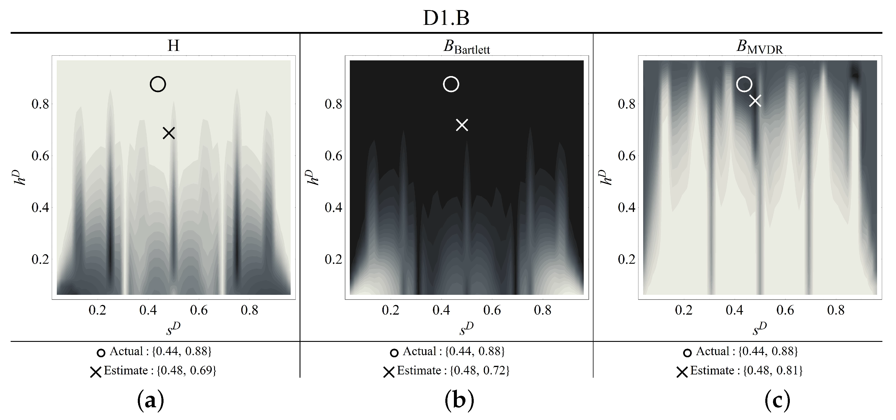
Figure 16.
Contour plots of the estimators for damage scenario D1.B ((a) objective function, (b) Bartlett, (c) MVDR) (thick circle: correct damage parameters; cross: identified parameters).
Figure 16.
Contour plots of the estimators for damage scenario D1.B ((a) objective function, (b) Bartlett, (c) MVDR) (thick circle: correct damage parameters; cross: identified parameters).
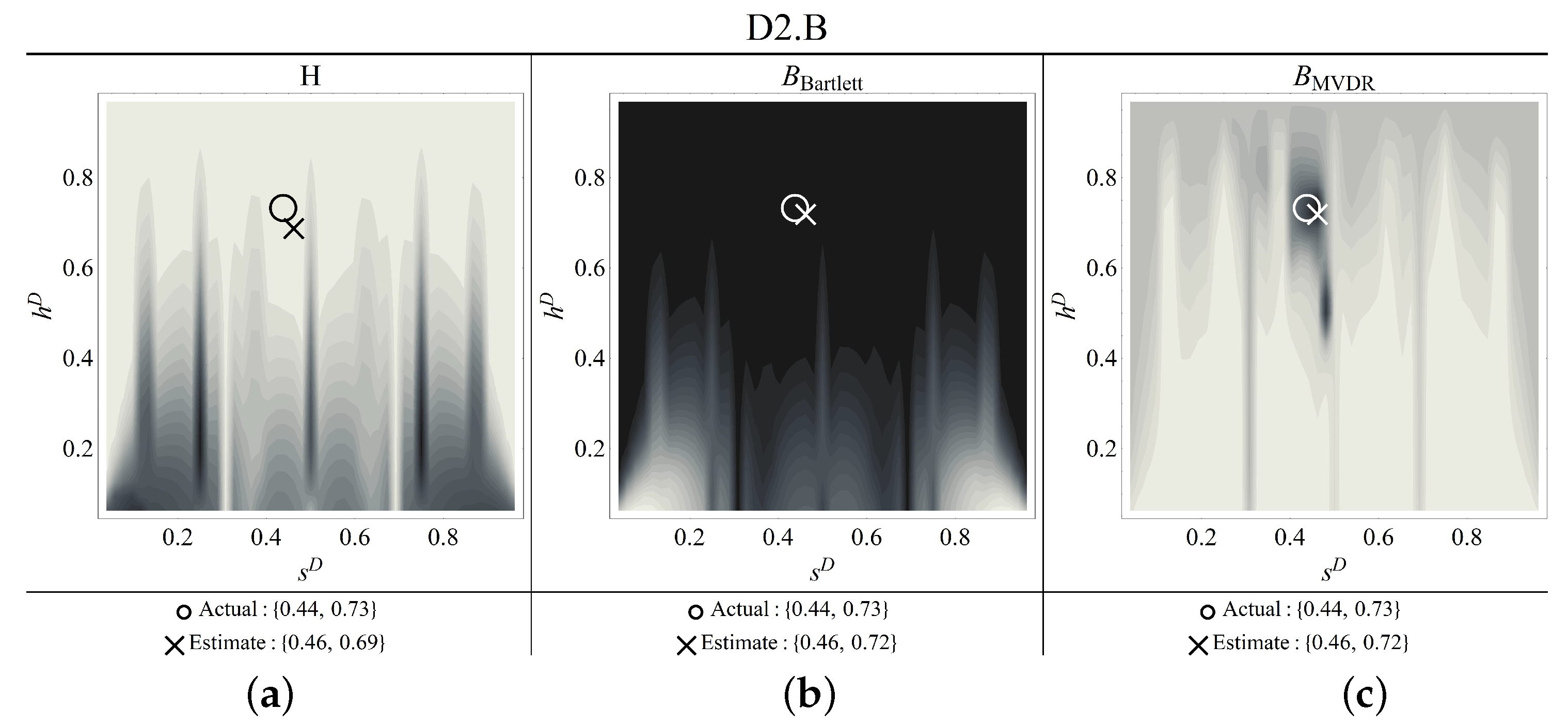
Figure 17.
Contour plots of the estimators for damage scenario D2.B ((a) objective function, (b) Bartlett, (c) MVDR) (thick circle: correct damage parameters; thin concentric circles: identified parameters).
Figure 17.
Contour plots of the estimators for damage scenario D2.B ((a) objective function, (b) Bartlett, (c) MVDR) (thick circle: correct damage parameters; thin concentric circles: identified parameters).
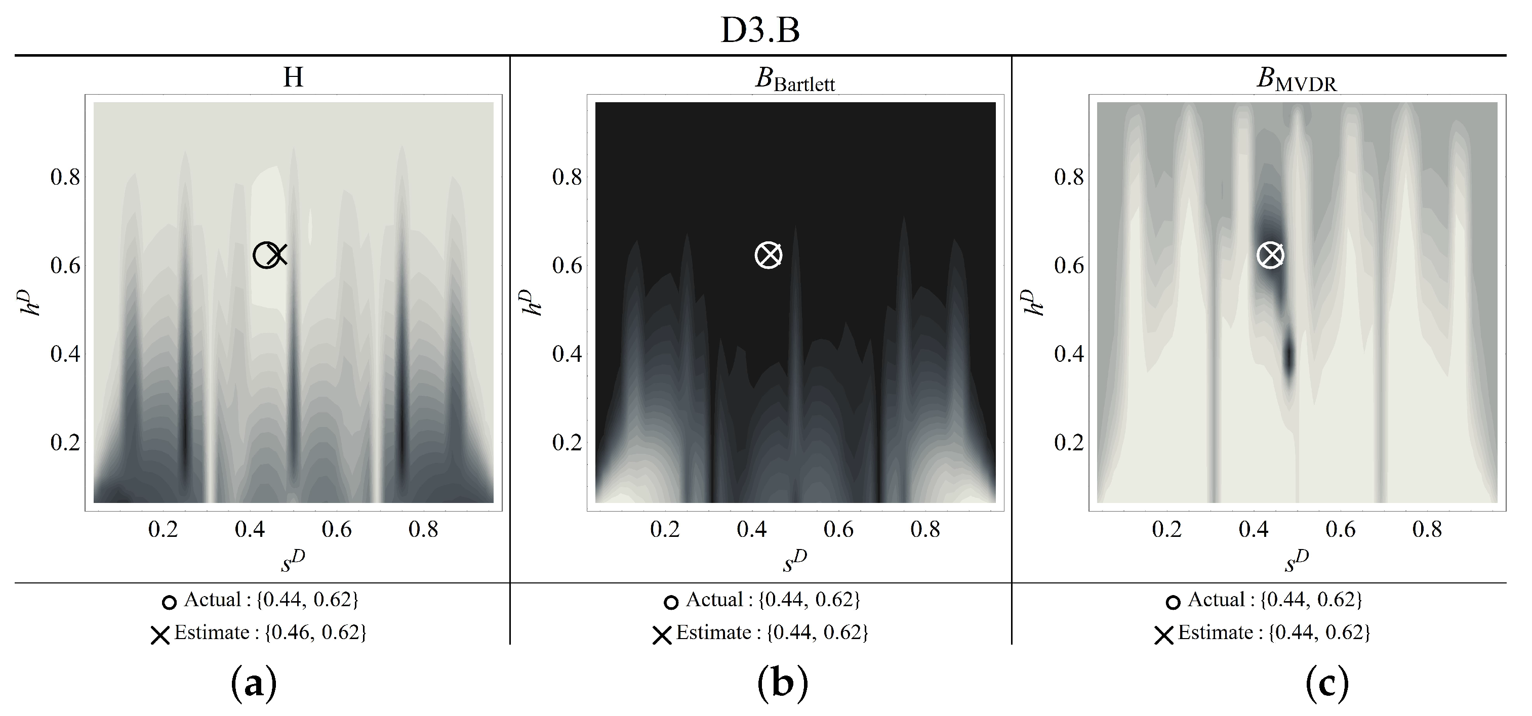
Figure 18.
Contour plots of the estimators for damage scenario D3.B ((a) objective function, (b) Bartlett, (c) MVDR) (thick circle: correct damage parameters; thin concentric circles: identified parameters).
Figure 18.
Contour plots of the estimators for damage scenario D3.B ((a) objective function, (b) Bartlett, (c) MVDR) (thick circle: correct damage parameters; thin concentric circles: identified parameters).
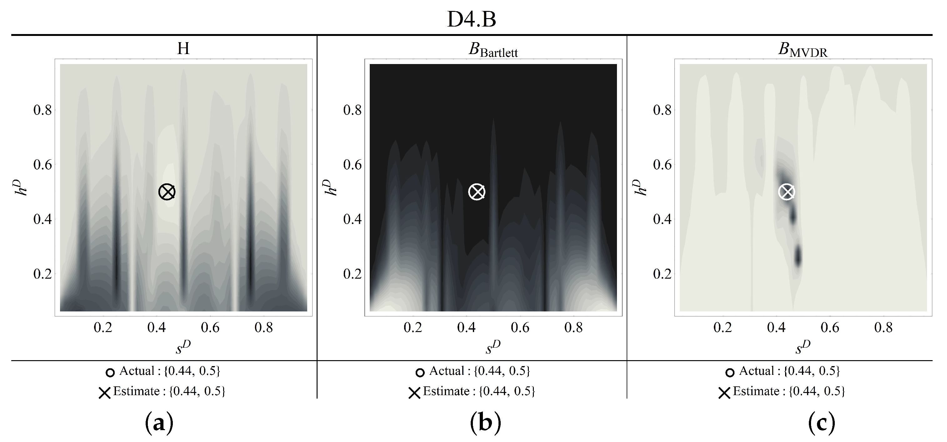
Figure 19.
Contour plots of the estimators for damage scenario D4.B ((a) objective function, (b) Bartlett, (c) MVDR) (circle: correct damage parameters; cross: identified parameters).
Figure 19.
Contour plots of the estimators for damage scenario D4.B ((a) objective function, (b) Bartlett, (c) MVDR) (circle: correct damage parameters; cross: identified parameters).
Table 1.
Labels of the damage scenarios with location (), nominal height of the damaged cross-section (), and percent stiffness reduction ().
Table 1.
Labels of the damage scenarios with location (), nominal height of the damaged cross-section (), and percent stiffness reduction ().
| | D1.A | D2.A | D3.A | D4.A | D1.B | D2.B | D3.B | D4.B |
|---|
| 0.25 | 0.25 | 0.25 | 0.25 | 0.4375 | 0.4375 | 0.4375 | 0.4375 |
| | | | | | | | |
| 33.0 | 57.8 | 75.6 | 87.5 | 33.0 | 57.8 | 75.6 | 87.5 |
Table 2.
Numerical natural frequencies () [Hz] of the first three modes () and their percent variation () due to damage.
Table 2.
Numerical natural frequencies () [Hz] of the first three modes () and their percent variation () due to damage.
| | U | D1.A | D2.A | D3.A | D4.A |
|---|
| 298.96 | 298.23 | 296.12 | 292.06 284.09 | |
| | 0.25 | 0.95 | 2.31 | 4.98 |
| 817.12 | 811.67 | 796.67 | 769.99 | 725.52 |
| | 0.67 | 2.50 | 5.77 | 11.21 |
| 1582.02 | 1572.86 | 1549.21 | 1512.15 | 1546.32 |
| | 0.58 | 2.07 | 4.23 | 7.39 |
| | U | D1.B | D2.B | D3.B | D4.B |
| 298.96 | 295.28 | 290.78 | 279.95 | 261.29 |
| | 1.23 | 2.73 | 6.36 | 12.60 |
| 817.12 | 810.97 | 809.69 | 800.44 | 785.54 |
| | 0.75 | 0.91 | 2.04 | 3.87 |
| 1582.02 | 1570.62 | 1568.89 | 1552.45 | 1525.23 |
| | 0.72 | 0.83 | 1.87 | 3.59 |
Table 3.
Damage scenarios with measured heights of the damaged cross section ( [mm]), and percent stiffness reduction ().
Table 3.
Damage scenarios with measured heights of the damaged cross section ( [mm]), and percent stiffness reduction ().
| | D1.A | D2.A | D3.A | D4.A | D1.B | D2.B | D3.B | D4.B |
|---|
| 13.3 | 11.3 | 9.6 | 7.6 | 13.2 | 11.0 | 9.4 | 7.5 |
| 30.3 | 57.2 | 73.8 | 87.0 | 31.9 | 60.6 | 75.4 | 87.5 |
Table 4.
Geometrical and mechanical properties of the beams used in cases A and B.
Table 4.
Geometrical and mechanical properties of the beams used in cases A and B.
| | H [mm] | B [mm] | [mm] | E [GPa] | [kg/m] |
|---|
| A | 15.40 | 30.12 | 130.0 | 206.5 | 7504.5 |
| B | 15.40 | 30.20 | 227.5 | 209.0 | 7656.8 |
Table 5.
Case A: experimental () and numerical () natural frequencies [Hz] of the first three modes (), and their percent variation (, ) due to damage.
Table 5.
Case A: experimental () and numerical () natural frequencies [Hz] of the first three modes (), and their percent variation (, ) due to damage.
| | | | | | | |
| U | 298.8 | | 813.52 | | 1589.8 | |
| D1.A | 298.2 | 0.21 | 810.5 | 0.38 | 1584.6 | 0.32 |
| D2.A | 296.8 | 0.68 | 797.8 | 1.98 | 1561.3 | 1.79 |
| D3.A | 294.1 | 1.58 | 784.5 | 3.57 | 1540.3 | 3.11 |
| D4.A | 288.7 | 3.40 | 753.2 | 7.41 | 1497.6 | 5.80 |
| | | | | | | |
| U | 298.8 | | 814.5 | | 1588.3 | |
| D1.A | 298.2 | 0.17 | 810.6 | 0.47 | 1581.8 | 0.41 |
| D2.A | 296.5 | 0.75 | 798.1 | 2.00 | 1561.6 | 1.68 |
| D3.A | 293.7 | 1.69 | 779.1 | 4.34 | 1533.5 | 3.45 |
| D4.A | 288.0 | 3.61 | 744.3 | 8.62 | 1489.4 | 6.23 |
Table 6.
Case B: experimental () and numerical () natural frequencies [Hz] of the first three modes (), and their percent variation (, ) due to damage.
Table 6.
Case B: experimental () and numerical () natural frequencies [Hz] of the first three modes (), and their percent variation (, ) due to damage.
| | | | | | | |
| U | 297.7 | | 809.8 | | 1584.5 | |
| D1.B | 295.5 | 0.73 | 808.3 | 0.19 | 1579.0 | 0.35 |
| D2.B | 287.8 | 3.33 | 803.5 | 0.78 | 1564.1 | 1.29 |
| D3.B | 282.1 | 5.23 | 799.0 | 1.34 | 1549.6 | 2.20 |
| D4.B | 267.6 | 10.12 | 790.0 | 2.45 | 1521.5 | 3.97 |
| | | | | | | |
| U | 297.5 | | 811.2 | | 1582.6 | |
| D1.B | 295.1 | 0.83 | 808.9 | 0.28 | 1578.7 | 0.26 |
| D2.B | 288.1 | 3.16 | 802.6 | 1.06 | 1567.5 | 0.96 |
| D3.B | 279.1 | 6.19 | 794.9 | 2.01 | 1553.5 | 1.85 |
| D4.B | 265.7 | 10.68 | 784.3 | 3.32 | 1534.2 | 3.06 |
Table 7.
Error % on the identified damage parameters for damage case A.
Table 7.
Error % on the identified damage parameters for damage case A.
| | D1.A | D2.A | D3.A | D4.A |
|---|
| | | | | | | | | |
| H | 100 | −12.7 | 0.0 | 6.9 | 0.0 | 11.3 | 0.0 | 14.3 |
| Bartlett | 0.0 | 5.8 | 0.0 | 6.9 | 0.0 | 11.3 | 0.0 | 14.3 |
| MVDR | 0.0 | 5.8 | 0.0 | 6.9 | 0.0 | 11.3 | 0.0 | 14.3 |
Table 8.
Error % on the identified damage parameters for damage case B.
Table 8.
Error % on the identified damage parameters for damage case B.
| | D1.B | D2.B | D3.B | D4.B |
|---|
| | | | | | | | | |
| H | 9.1 | −21.6 | 4.6 | −5.5 | 4.6 | 0.0 | 0.0 | 0.0 |
| Bartlett | 9.1 | −18.2 | 4.6 | −1.4 | 0.0 | 0.0 | 0.0 | 0.0 |
| MVDR | 9.1 | −8.0 | 4.6 | −1.4 | 0.0 | 0.0 | 0.0 | 0.0 |


