Multi-Scale Concurrent Topology Optimization Based on BESO, Implemented in MATLAB

Abstract

In multi-scale topology optimization methods, the analysis encompasses two distinct scales: the macro-scale and the micro-scale. The macro-scale refers to the overall size and dimensions of the structural domain being studied, while the micro-scale pertains to the periodic unit cell that constitutes the macro-scale. This unit cell represents the entire structure or component targeted for optimization. The primary objective of this research is to present a simplified MATLAB code that addresses the multi-scale concurrent topology optimization challenge. This involves simultaneously optimizing both the macro-scale and micro-scale aspects, taking into account their interactions and interdependencies. To achieve this goal, the proposed approach leverages the Bi-directional Evolutionary Structural Optimization (BESO) method. The formulation introduced in this study accommodates both cellular and composite materials, dealing with both separate volume constraints and the utilization of a single volume constraint. By offering this simplified formulation and harnessing the capabilities of the multi-scale approach, the research aims to provide valuable insights into the concurrent optimization of macro- and micro-scales. This advancement contributes to the field of topology optimization and enhances its applications across various engineering disciplines.

1. Introduction

A topology optimization problem formulation can be adopted to determine the optimal geometry for either the structural domain, the material, or both, with the objective of minimizing, e.g., structural compliance while considering a specific volume fraction. The structural domain involved in such a problem consists of a periodically repeated cellular material, which is represented by a unit cell. To solve these types of Topology Optimization (TO) problems, two approaches are commonly employed: the mono-scale approach and the multi-scale approach. In the multi-scale approach, establishing a connection between the different scales can be achieved through various methodologies. One popular method is the utilization of the Homogenization method. This technique enables the translation of the periodic unit cell geometry into a homogenized elasticity tensor, which can then be employed in the finite element analysis of the structural domain. The theoretical foundations of the homogenization methodology were initially presented by Bensoussan and Lions in [1] and Sanchez-Palencia in [2]. The process of numerical homogenization involves implementing the homogenization theory using finite elements and the finite element analysis method to compute the homogenized elasticity tensor. Further insights into numerical homogenization can be found in the works of Guedes and Kikuchi in [3] as well as Hassani and Hinton in [4,5,6]. The homogenization theory has been effectively employed to solve the TO formulation in the context of homogenization-based TO problems, as demonstrated by Bendsøe and Kikuchi in [7]. Moreover, Arabnejad and Pasini in [8] utilized homogenization to compute the mechanical properties of various periodic unit cells with different relative densities. Notably, numerical implementations of the homogenization method in the form of MATLAB codes have been provided by Andreassen and Andreasen in [9] for 2D spaces and by Dong et al. in [10] for 3D spaces. These resources offer practical tools for applying the homogenization method in topology optimization.

The optimization procedure of the multi-scale TO problem formulation can be implemented in either hierarchical or concurrent form. In the case of the hierarchical implementation, introduced by Rodrigues et al. in [11] the optimization procedure consists of two separate problems, the inner and outer problem. In the inner problem, the geometry of the unit cell is optimized for a fixed structural domain. In the outer problem, the geometry of the structural domain is optimized for a fixed periodic unit cell. Thus, at every optimization step, the inner and outer problems are solved hierarchically, providing each other with new geometries. In the concurrent optimization procedure, the geometries of the micro and macro-scales are updated simultaneously, like the procedure presented by Liu et al. in [12]. This is achieved by augmenting the TO problem with the two sets of design variables representing the two different scales. The first set of design variables consists of the relative material densities of the finite elements discretizing the structural domain, whereas the second set of design variables consists of the relative material densities of the finite elements discretizing the periodic unit cell. Thus, in the presented methodology, the periodic unit cell geometry is optimized by directly changing all parts of the unit cell geometry through the assigned material densities. To gain additional insights into the multi-scale TO formulations, readers are encouraged to refer to the review published by Wu et al. in [13].

The solution of the concurrent multi-scale TO formulation is based on the BESO approach. BESO in contrast to the popular SIMP approach is based on the discrete implementation of the TO problem and is categorized as a soft-kill approach. The BESO-based TO optimization approach was based on the Evolutionary Structural Optimization (ESO) approach, which was first introduced by Xie and Steven in [14,15,16]. The focus of the ESO-based TO problem was to slowly remove elements from the structural domain during the optimization procedure. The initial main criterion for the element removal was set as the stress field. Chu et al. in [17] proposed a change in the criterion from stress to strain energy. The modified version of ESO called the BESO approach was proposed by Querin et al. in [18,19] in which new elements can be added by the algorithm. To avoid completely removing elements during the optimization procedure, a soft-BESO approach is proposed. Zhu et al. in [20] and Huang and Xie in [21] utilized material interpolation schemes similar to the Solid Isotropic Material with Penalization (SIMP) to include the soft elements during the optimization procedure. The soft-kill version of BESO combined with a modified version of SIMP is utilized in the presented implementation. Regarding multi-scale concurrent topology optimization (TO) and optimal material design, several notable studies have been conducted. Huang et al. in [22,23] introduced a formulation for optimal material design encompassing cellular and composite materials, employing the BESO approach. In a similar vein, Yan et al. in [24] proposed a concurrent multi-scale TO formulation utilizing the BESO approach for both macro and micro-scales, employing composite microstructures of two-phase materials. Furthermore, Xu et al. in [25] presented a formulation concerning multi-scale TO based on the BESO approach, utilizing dynamic compliance as the objective function for the formulation.

Regarding the TO formulation, many different code implementations have been published. The first code implementation was published by Sigmund in [26] and is referred to as top99, 99 lines of MATLAB code for the SIMP-based TO formulation in 2D. The top99 was later formatted to the top88, 88 lines of MATLAB code published by Andreassen et al. in [27]. Later, the top99 code was expanded to the 3D space by Liu and Tovar in [28] and a more optimized version for both 2D and 3D by Ferrari et al. in [29]. Based on the SIMP MATLAB implementations, Huang and Xie in [30] published a BESO-based TO MATLAB implementation for the 2D space. Based on the homogenization method and their MATLAB implementations mentioned above, Xia and Breitkopf in [31] as well as Kazakis and Lagaros in [32,33] presented MATLAB implementations for the optimal design of materials using the TO formulation. In these implementations, only the geometry of the periodic unit cell was optimized. Lastly, Gao et al. [34] presented a MATLAB implementation for the multi-scale concurrent TO formulation based on the SIMP approach.

In this optimization problem, the structural domain consists of periodically repeated cellular material in the form of a unit cell. Thus, the focus of the optimization procedure is to find the optimal geometry of both structure and material for minimizing the structural compliance for a given volume fraction. These types of Topology Optimization (TO) problem formulations can be solved using two different approaches, the mono-scale and multi-scale approach. In the mono-scale approach, only one scale is considered for the optimization procedure, whereas in the multi-scale approach, typically two different scales are considered for the optimization procedure. These scales consist of the macro-scale and micro-scale. The macro-scale refers to the scale of the structural domain, whereas the micro-scale refers to the scale of the periodically repeated unit cell representing the cellular material. The main objective of this work is to present a simple formulation for the multi-scale concurrent topology optimization problem based on the Bi-directional Evolutionary Structural Optimization (BESO) approach. In the presented formulation, the multi-scale approach will be implemented for the solution of the optimization procedure.

This study is structured into seven sections, together with the Introduction and Conclusions sections. The mathematical problem formulation for the concurrent multi-scale topology optimization (TO) is presented in Section 2. The sensitivity analysis of the objective function for the two sets of design variables is detailed in Section 3, building upon the mathematical formulation. The implementation of the BESO approach is explained in Section 4, and subsequent to that, the MATLAB implementation for both 2D and 3D design domains is provided in Section 5. Various numerical examples demonstrating the presented methodology are showcased in Section 6, and Section 7 delves into the extensions necessary for dealing with two-phase composite materials, along with additional numerical examples.

2. Multi-Scale Topology Optimization—Problem Formulation

Since the optimization problem formulation, involves both scales (structure and periodic unit cell) the design variables, i.e., relative densities are applied in both scales. Thus, similarly to the classic TO formulation, the relative material densities applied to the finite elements discretizing the macro domain (structure) are presented as x, whereas the relative densities applied to the finite elements discretizing the microdomain (periodic unit cell) are presented as y. In addition, to separate the indicators of the two sets of finite elements (of the macro and micro-scale), the indicator for the finite elements discretizing the macro domain is e whereas the indicator for the finite elements discretizing the microdomain is $el$. Hence, $x_e$ refers to the relative density of a finite element of the macro domain and $y_{el}$ refers to the relative density of a finite element of the microdomain. The mathematical formulation of the optimization problem follows the expression of Equation (1).

$$\begin{gathered} \begin{array}{cc}\hfill \underset{x,y}{min}C(x,y)& =F^T·U(x,y)\hfill \end{array} \\ s.t. \\ \begin{array}{cc}\hfill F& =K(x,y)·U\hfill \\ \hfill V\left(x\right)/V_x& =f_x\hfill \\ \hfill V\left(y\right)/V_y& =f_y\hfill \\ \hfill 0\le & x_e\le 1\hfill \\ \hfill 0\le & y_{el}\le 1\hfill \end{array} \end{gathered}$$

(1)

where the term $C(x,y)$ refers to the structural compliance that was chosen as the objective function to be optimized. The terms F and U refer to the loading vector and the resulting displacement field, respectively. The equation $F=K·U$ refers to the equilibrium equation, which is solved using the finite element method (FEM). The terms $V\left(x\right)$ and $V\left(y\right)$ refer to the volumes of the structure and periodic unit cell, respectively. Similarly, the terms $V_x$ and $V_y$ refer to the volumes of the whole structure and periodic unit cell, respectively. The volume fractions for the two scales which are the target volumes for the final optimal designs are referred to as $f_x$ and $f_y$ for the macro and micro-scale, respectively. Lastly, as mentioned at the beginning of this section, $x_e$ and $y_{el}$ refer to the relative material densities for the macro and micro-scale, respectively. Similarly to the classic TO formulation, the relative densities of both scales are bounded between the values of zero and one.

As illustrated in the equilibrium equation, the two groups of material densities have a notable impact on the global stiffness matrix values. This influence stems from the definition of the elemental stiffness matrices denoted as $k_e$ for each individual element e. These element stiffness matrices $k_e$ for each finite element e conform to the expression provided in Equation (2).

$$k_e(x,y)=E_e\left(x\right)·k_e^H\left(y\right)$$

(2)

where term $E\left(x\right)$ refers to the influence of the relative material density $x_e$ and term $k_e^H\left(y\right)$ refers to the homogenized element stiffness matrix. The influence of the material density $x_e$ is implemented using the modified SIMP approach [35]. Using the modified SIMP approach, the zero-based material densities are assigned a minimum value to avoid zero-valued stiffness matrices. The penalization term has no meaningful effect in our case but is included to keep the expression similar to the modified SIMP. Thus, the term $E\left(x\right)$ follows the expression of Equation (3).

$$E_e\left(x\right)=x_e^p·(1-x_{min})+x_{min}$$

(3)

where $x_{min}$ refers to a minimum value for the influence term to avoid zero values and the term p refers to the SIMP penalization factor. The homogenized element stiffness matrix $k_e^H$ is only a function of the material densities y through the elasticity tensor. Hence, the term $k_e^H$ follows the typical expression of a Q4 finite element stiffness matrix, i.e., the expression of Equation (4).

$$k_e^H\left(y\right)={\int }_{V_e}(B_e^T·C^H\left(y\right)·B_e)d{V}_e$$

(4)

where $B_e$ refers to the strain-displacement matrix and $C^H$ refers to the homogenized elasticity tensor. Due to the macrostructure consisting of only one type of periodic unit cell, the homogenized elasticity tensor is the same for all finite elements e. To obtain the values of the homogenized elasticity tensor, $C^H$ the theory of numerical homogenization is utilized. According to numerical homogenization, the term $C^H$ follows the expression of Equation (5).

$$C^H\left(y\right)=\frac{1}{V_y}\sum _{el=1}^{n_{el}}{\int }_{V_{el}}(u_{el}^0-u_{el})·k_{el}\left(y\right)·(u_{el}^0-u_{el})d{V}_{el}$$

(5)

where $n_{el}$ refers to the number of finite elements $el$. From the theory of homogenization, the terms $u_{el}^0$ and $u_{el}$ refer to the displacement fields resulting from the globally (in the unit cell) applied unit strains and the element application of the unit strains, respectively. Lastly, the term $k_{el}$ refers to the element stiffness matrix of the elements $el$. Similarly to the element stiffness matrix for the finite elements e, the term $k_{el}$ follows the expression of Equation (6).

$$k_{el}\left(y\right)=E_{el}\left(y\right)·k_0$$

(6)

where the term $E_{el}$ refers to the Young’s modulus of the finite element $el$ as a function of the material density y and the term $k_0$ refers to the elemental stiffness matrix for an element with a unit Young’s modulus ($E=1$). Similarly to the macro-scale, the value of the term $E_{el}$ is obtained using the modified SIMP approach [35]. Therefore, the term $E_{el}$ is obtained following the expression of Equation (7).

$$E_{el}\left(y\right)=E_{min}+y_{el}^p·(E^0-E_{min})$$

(7)

where the term $E^0$ refers to the material Young’s modulus and the term $E_{min}$ refers to a minimum value of the Young’s modulus to avoid zero Young’s modulus values. Similarly to Equation (3), in Equation (7) the penalization term can be omitted but is included to retain the modified SIMP expression.

3. Sensitivity Calculations for Concurrent Multi-Scale Expressions

In this part of the study, the sensitivity analysis of the concurrent multi-scale TO formulation is presented. Due to the two different sets of material densities, the sensitivity of the compliance is obtained through two different expressions. Hence, the sensitivity of the objective function with respect to the two sets of material densities x and y follows the expressions of Equation (8).

$$\begin{array}{cc}\hfill \frac{\partial C}{\partial x_e}& =-U_e^T·\frac{\partial k}{\partial x_e}·U_e\hfill \\ \hfill \frac{\partial C}{\partial y_{el}}& =-\sum _{e=1}^{N_e}{U}_e^T·\frac{\partial k}{\partial y_{el}}·U_e\hfill \end{array}$$

(8)

where the term $U_e$ refers to the displacement field of element e and the term $N_e$ refers to the number of elements e. For the case regarding the material densities, x the sensitivity of the objective function requires the sensitivity of the element stiffness matrix $\partial k/\partial x_e$. The sensitivity of the element stiffness matrix is obtained by differentiating the expression of Equation (2) with respect to $x_e$. Hence, the term $\partial k/\partial x_e$ follows the expression of Equation (9).

$$\frac{\partial k}{\partial x_e}=\frac{\partial E}{\partial x_e}·k_e^H$$

(9)

The term $k_e^H$ is only a function of, y and thus is not affected by the differentiation. To obtain the value of the term $\partial E/\partial x_e$, the expression of Equation (3) is differentiated as well. Thus, the term $\partial E/\partial x_e$ is obtained following the expression of Equation (10).

$$\frac{\partial E}{\partial x_e}=p·x_e^{p-1}·(1-x_{min})$$

(10)

Moving to the second set of objective function sensitivities, the sensitivity of the objective function with respect to the y set of material densities requires the sensitivity of the stiffness matrix $\partial k/\partial y_{el}$. The term $\partial k/\partial y_{el}$ can be obtained by differentiating the expression of Equation (2) with respect to $y_{el}$. Hence, the term $\partial k/\partial y_{el}$ is obtained following the expression of Equation (11).

$$\frac{\partial k_e}{\partial y_{el}}=E_e\left(x\right)·\frac{\partial k_e^H}{\partial y_{el}}$$

(11)

Here, the term $E_e\left(x\right)$ is not a function of y and thus is not affected by the differentiation. The derivative of the homogenized stiffness matrix with respect to y is obtained by differentiation of the expression of Equation (4). Therefore, the term $\partial k_e/\partial y_{el}$ is obtained following the expression of Equation (12).

$$\frac{\partial k_e^H}{\partial y_{el}}={\int }_{V_e}(B_e^T·\frac{\partial C^H}{\partial y_{el}}·B_e)d{V}_e$$

(12)

The derivative of the homogenized elasticity tensor with respect to y is obtained by differentiation of the expression of Equation (5). Consequently, the term $\partial C^H/\partial y_{el}$ is obtained following the expression of Equation (13).

$$\frac{\partial C^H}{\partial y_{el}}=\frac{1}{V_y}\sum _{i=1}^{n_{el}}{\int }_{V_{el}}(u_{el}^0-u_{el})·\frac{\partial k_{el}}{\partial y_{el}}·(u_{el}^0-u_{el})d{V}_{el}$$

(13)

The derivative of the element stiffness matrix with respect to y is obtained by differentiation of the expression of Equation (6). Hence, the term $\partial k/\partial y_{el}$ is obtained following the expression of Equation (14).

$$\frac{\partial k}{\partial y_{el}}=\frac{\partial E}{\partial y_{el}}·k_0$$

(14)

The term $k_0$ is not a function of y and thus is not affected in the differentiation. The final part of the sensitivity analysis is to obtain the derivative of the material Young’s modulus with respect to y. Thus, the term $\partial E/\partial y_{el}$ is obtained following the expression of Equation (15).

$$\frac{\partial E}{\partial y_{el}}=p·y_{el}^{p-1}·(E^0-E_{min})$$

(15)

4. BESO Implementation of Concurrent Treatment of the Multi-Scale Problem

The BESO approach is a discrete-based approach that uses a specified value for each element as an indicator of the element’s existence. This indicator is generally called sensitivity number and is based on the element’s sensitivity. In this section, the general idea of the soft-BESO approach will be presented first, and then it will be expanded for the concurrent multi-scale TO formulation. In the general representation, the indicator x will be used as an indicator for the material densities due to the classic form of the TO problem formulation. The general form of the sensitivity number of an element a of the soft version of BESO is obtained following the expression of Equation (16).

$$a_e=-\frac{1}{p}·\frac{\partial C}{\partial x_e}$$

(16)

whereas described in the previous section, the term $\partial C/\partial x_e$ refers to the sensitivity of the objective function and the term p refers to the penalty factor. Due to BESO being a discrete approach for the TO problem, material densities x are allowed to only take the values of zero or one. The mapping of the material densities is achieved using the sensitivity numbers of each finite element. A threshold value $a_x$ for the sensitivity numbers is usually used in the mapping procedure. Thus, utilizing the sensitivity numbers as well as the threshold value, $a_x$ the mapping procedure follows the expression of Equation (17).

$$x_e=\left\{\begin{array}{cc}1\hfill & for{a}_e\ge a_x\hfill \\ 0\hfill & for{a}_e<a_x\hfill \end{array}\right.$$

(17)

The specification of the value of the sensitivity number threshold $a_x$ is achieved using the expression of Equation (17) and performing a search for the threshold value that satisfies the volume constraint imposed onto the classic TO optimization problem. The elemental Young’s modulus can be obtained by combining the modified SIMP approach [35] and the expression of Equation (17). Hence, the mapping of the Young’s modulus using the threshold sensitivity number follows the expression of Equation (18).

$$E_e=\left\{\begin{array}{cc}(E^0-E_{min})\hfill & for{a}_e\ge a_x\hfill \\ E_{min}\hfill & for{a}_e<a_x\hfill \end{array}\right.$$

(18)

Thus, using the modified SIMP approach, there is no element removal during the optimization procedure. Alternatively, elements with zero-valued material densities are assigned with a very small Young’s modulus, making the optimization procedure more stable. To stabilize the optimization procedure even more in general the volume constraint is not applied at once. In contrast, the volume constraint is gradually imposed onto the optimization procedure, with the target volume usually initializing at $100\%$ and gradually decreasing at every optimization step. The rate of decrease is generally a parameter of the optimization procedure and can affect the stability of the optimization.

Moving to the presented formulation, the general idea of the soft-BESO implementation remains the same as in the classic TO formulation presented above. In this case, due to the two sets of material densities and by extension sensitivities of the objective function and constraints, the BESO implementation is basically applied separately at each set. Thus, the sensitivity numbers are obtained by applying the expression of Equation (16) to the new formulation and following the expressions of Equation (19).

$$\begin{array}{cc}\hfill a_e& =-\frac{1}{p}·\frac{\partial C}{\partial x_e}\hfill \\ \hfill a_{el}& =-\frac{1}{p}·\frac{\partial C}{\partial y_{el}}\hfill \end{array}$$

(19)

Due to the two different volume constraints (one for each scale), the threshold for the sensitivity numbers is two $a_x$ for the macro-scale and $a_y$ for the micro-scale. As described in the general implementation of the soft-BESO approach, the values of the two threshold numbers are obtained using the two different volume constraints and the expression of Equation (17) implemented for the material densities x and y. Hence, to obtain the elemental Young’s modulus for the micro-scale as well as the term $E_x$ for the macro-scale, the expression of Equation (18) is modified following the expressions of Equations (3) and (7). Therefore, the term $E_x$ is obtained following the expression of Equation (20).

$$E_e=\left\{\begin{array}{cc}(1-x_{min})\hfill & for{a}_e\ge a_x\hfill \\ x_{min}\hfill & for{a}_e<a_x\hfill \end{array}\right.$$

(20)

and the Young’s modulus of each finite element $el$ is obtained following the expression of Equation (21).

$$E_{el}=\left\{\begin{array}{cc}(E^0-E_{min})\hfill & for{a}_{el}\ge a_y\hfill \\ E_{min}\hfill & for{a}_{el}<a_y\hfill \end{array}\right.$$

(21)

5. MATLAB Implementation

In this section, a MATLAB implementation of the multi-scale concurrent formulation is presented for both 2D and 3D design spaces. The MATLAB code for the 2D implementation is based on the optimal material design MATLAB codes presented by Kazakis and Lagaros in [32] as well as the $top88$ MATLAB code presented by Andreassen et al. in [27] and the MATLAB implementation of the soft-BESO approach presented by Huang and Xie in [30]. For the 3D MATLAB implementation, the code is based on the optimal material design using TO in 3D presented by Kazakis and Lagaros in [33] as well as the top3D MATLAB code presented by Liu and Tovar in [28] and the soft-BESO implementation mentioned above. For the homogenization method, modified implementations of the MATLAB codes presented by Andreassen and Andreasen in [9] and Dong et al. in [10] for 2D and 3D space, respectively.

5.1. MATLAB Implementation for 2D Design Space

The UCOpt MATLAB function developed for the optimal material design using TO [32] was used as the basis for the multi-scale concurrent MATLAB code presented in the current section. Thus, only the parts of the MATLAB code modified will be highlighted. The name of the new MATLAB function for solving the multi-scale concurrent TO problem formulation is set as ConcTopOptBESO.

The first set of modifications is focused on the input and output parameters. The volume target variable $volfrac$ of the original UCOpt function is changed to take into account the two different volume constraints applied to the optimization problem. Thus, $volfrac$ is modified into $volfx$ and $volfy$ as the target volume fractions of the macro and micro-scales, respectively. Similarly, the filtering radius variable $rmin$ is modified into two different variables named $rxmin$ and $rymin$. The first variable is utilized for the filtering of the sensitivities of the macro-scale whereas the second variable is utilized for the filtering of the sensitivities of the micro-scale. Parameter $ft$ is due to the filtering application on only the sensitivity number, with no density filtering available. An additional variable is added to the input parameters of the ConcTopOptBESO MATLAB function called $er$. As described in [30], the $er$ variable is the evolutionary rate of the two target volumes. Regarding the output parameters, the final geometries of the macro and micro-scales as well as the homogenized elasticity matrix are added in the form of the variables $x,y$ and $CH$, respectively. Hence, the final form of the input function is formulated following Listing 1.

Listing 1 Input and output parameters of the main function for the 2D problem

At the beginning of the new function, in addition to the initialization of the variables $E0,Emin$ and $nu$, an extra variable $xmin$ is initialized for the later implementation of the expression of Equation (3). The value of $xmin$ is set as a small number, in this case $1e-8$. In the case of the multi-scale concurrent TO, the topology optimization is performed in both the macro and micro-scales. Thus, two different sets of material densities are implemented, one for the macro and one for the micro-scale. To distinguish between the two sets, a different variable is assigned to each set. The variable x is set for the macro-scale material densities and the variable y is set for micro-scale material densities. The MATLAB function UCOpt was formulated to perform the optimal material design using TO in the micro-scale. Hence, to formulate the two different sets of material densities, all instances of the variable x in the original UCOpt function are modified to y.

Moving to the preparation of the filtering matrices and the initialization sections, two different filtering matrices in the form of $Hx,Hsx$ and $Hy,Hsy$ are computed for the macro and micro-scale, respectively. The procedure for computing both sets is identical, with the only difference in the filtering radius considered for each scale ($rxmin$ for the macro and $rymin$ for the micro-scale, respectively). In the initialization section, in addition to the initialization of the y variable, the x variable is initialized following Listing 2.

Listing 2 Initialization of x variable

For the initialization of matrix y, in the original UCOpt function and rectangle mesh was set with a hole at its center. An Additional, initialization can include the set of ones to all y values. Furthermore, two new variables are implemented called $volx$ and $voly$, and initialized at one. Similarly to the code provided in [30], variables $volx$ and $voly$ represent the current volume fraction target of each iteration for the macro and micro-scale, respectively.

Moving inside the optimization procedure, an extra step is added at the beginning of the optimization iteration. In this step, the iterations target volume fractions for each scale are computed utilizing the evolutionary rate parameter. Hence, the final form of the optimization step is formulated following Listing 3.

Listing 3 Update scheme for the two target volumes

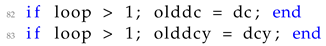
After the volume update step and following the sensitivity filtering implementation presented in [30], each iteration’s sensitivity values are stored for both scales using the following $Lines$ presented in Listing 4.

Listing 4 Saving of sensitivities of previous optimization iteration

In the finite element analysis step, $Line$ 90 is modified according to the expression of Equation (3). Hence, $Line$ 90 is formulated following Listing 5.

Listing 5 Computation of element stiffnesses into the sK variable

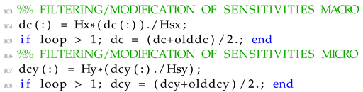
The sensitivity analysis step of the optimization procedure is modified; thus, both sets of sensitivities are computed. For the macro set of sensitivities, the code implementation follows the top88 implementation presented in [27]. For the micro set of sensitivities, the code implementation follows the original UCOpt function, utilizing the cellfun MATLAB function to eliminate the need for the double loop implemented in UCOpt. The filtering of sensitivities step of the optimization procedure is modified, performing only the option 2 of the original UCOpt function for both scales. In addition, as suggested in [30] the sensitivities are averaged between the two last iterations. The whole filtering step of the optimization procedure is implemented following Listing 6.

Listing 6 Filtering of sensitivities for the micro and macro scales

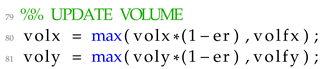
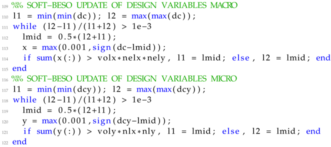
The last step of the optimization procedure is the BESO update scheme. As presented in [30], the BESO update scheme utilizes the sensitivities and the iteration target volumes calculated in the previous steps to produce the new set of material densities. The update scheme is implemented separately for the macro and micro-scales following Listing 7.

Listing 7 Update of design variables for the micro and macro scales

Lastly, due to the discrete nature of the material densities, the convergence criterion is modified from the maximum change in the material density values to the change in the objective function values.

5.2. MATLAB Implementation for 3D Design Space

The MATLAB implementation of the 3D multi-scale concurrent TO formulation was based on the UCOpt3D MATLAB function published by Kazakis and Lagaros in [33]. Hence, similarly to the 2D implementation presented in the previous subsection, only the parts modified to formulate the new optimization problem will be presented in the current subsection. In addition, the name of the new MATLAB function is set as ConcTopBeso3D.

The first set of modifications is on the input and output parameters of the original UCOpt3D function. The modifications are similar to the ones presented in the 2D version. Thus, due to the two different scales present in the multi-scale optimization procedure, variables $volfrac$ as well as $rmin$ are replaced with $volfx,volfy$ and $rxmin,rymin$, respectively. Variables $volfx$ and $volfy$ refer to the target volume fractions of the macro and micro-scale, respectively. Likewise, variables $rxmin$ and $rymin$ refer to the filter radius of the macro and micro-scale, respectively. Additionally, the BESO evolutionary rate is added in the form of the variable $er$ and in this case the second Model Order Reduction Model (MOR) is removed with the MOR applied only in the finite element analysis of the macro-scale. Furthermore, four different output variables are set as $c,CH,x$ and y referring to the compliance, homogenized elasticity tensor, and material densities of the macro and micro domain, respectively. Hence, the final form of the input function is formulated following Listing 8.

Listing 8 Input and output parameters of the main function for the 3D problem

Due to the UCOpt3D MATLAB function implementing the optimal material design using TO, the x variable refers to the material densities of the micro-scale. Thus, in the ConcTopBeso3D implementation, all references to x are modified as y. In addition to the initialization of the material parameters, an extra variable is added, set as $xmin$, which represents the minimum value presented in the expression of Equation (3). Moving to the filtering and initialization sections, matrices $H,Hs$ are initialized for both the macro and micro-scale using the same procedure utilized in the UCOpt3D MATLAB function. In the initialization section, in addition to the initialization of the material densities of the micro-scale, the material densities of the macro-scale are set to have a value of one. Furthermore, the variables $volx,voly$ representing the target volume fraction for each iteration for the macro and micro-scale, respectively, are also initialized to one.

Inside the optimization procedure, the modifications mirror the ones made in the 2D implementation. Thus, an extra step for the update of the target volume fractions is added at the start of the optimization procedure. Furthermore, the creation of the vector $sK$ used in the construction of the global stiffness matrix is modified according to the expression of Equation (3) and thus formulated following Listing 9.

Listing 9 Computation of element stiffnesses into the sK variable

In the sensitivity analysis step, the sensitivity of the macro-scale is computed following the implementation of the top3d presented in [28] whereas the sensitivity of the micro-scale is computed following the existing implementation of the original UCOpt3D function. In the filtering of the sensitivities, the filtering procedure follows the second option of the original UCOpt3D function and similarly to the 2D implementation, an average of the two last iterations is considered for the sensitivities. Regarding the BESO update scheme implementation, similarly to the 2D version, the new sets of material densities are computed separately. The code of the implementation of the BESO update scheme remains the same as the one implemented in the 2D version, due to the use of the MATLAB matrices.

6. Numerical Results

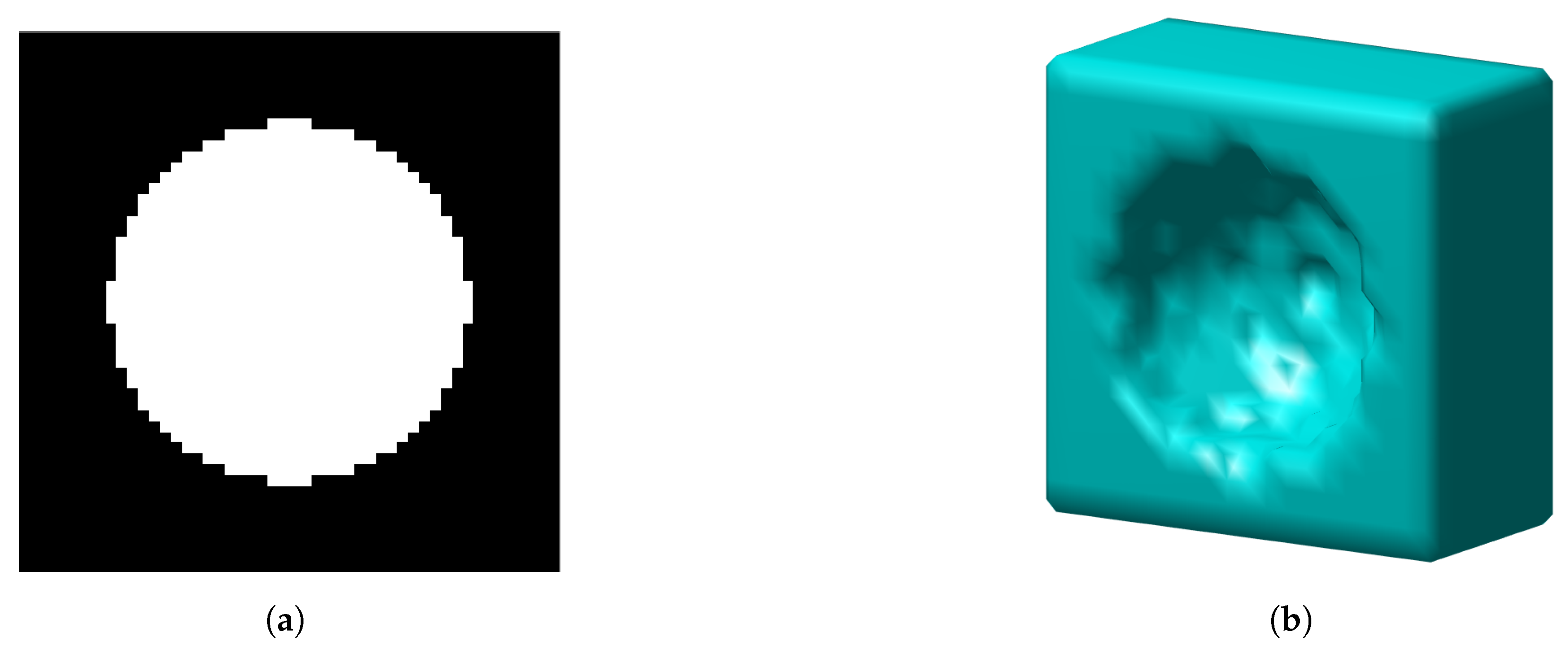
In this section, different test cases regarding the presented formulation are illustrated in both 2D and 3D space. All test cases are taken from the literature and illustrate different applications of the presented formulation. In all test cases, the final geometry of both the macro and micro-scales is presented. The starting material densities for all test cases regarding the macro-scale were set equal to the volume fraction target value. In the micro-scale, the starting geometry was set as a solid domain with a hole at the center of the unit cell and a radius of $1/3$ the dimensions of the periodic unit cell. A graphical representation of the unit cell geometry for both 2D and 3D is presented in Figure 1.

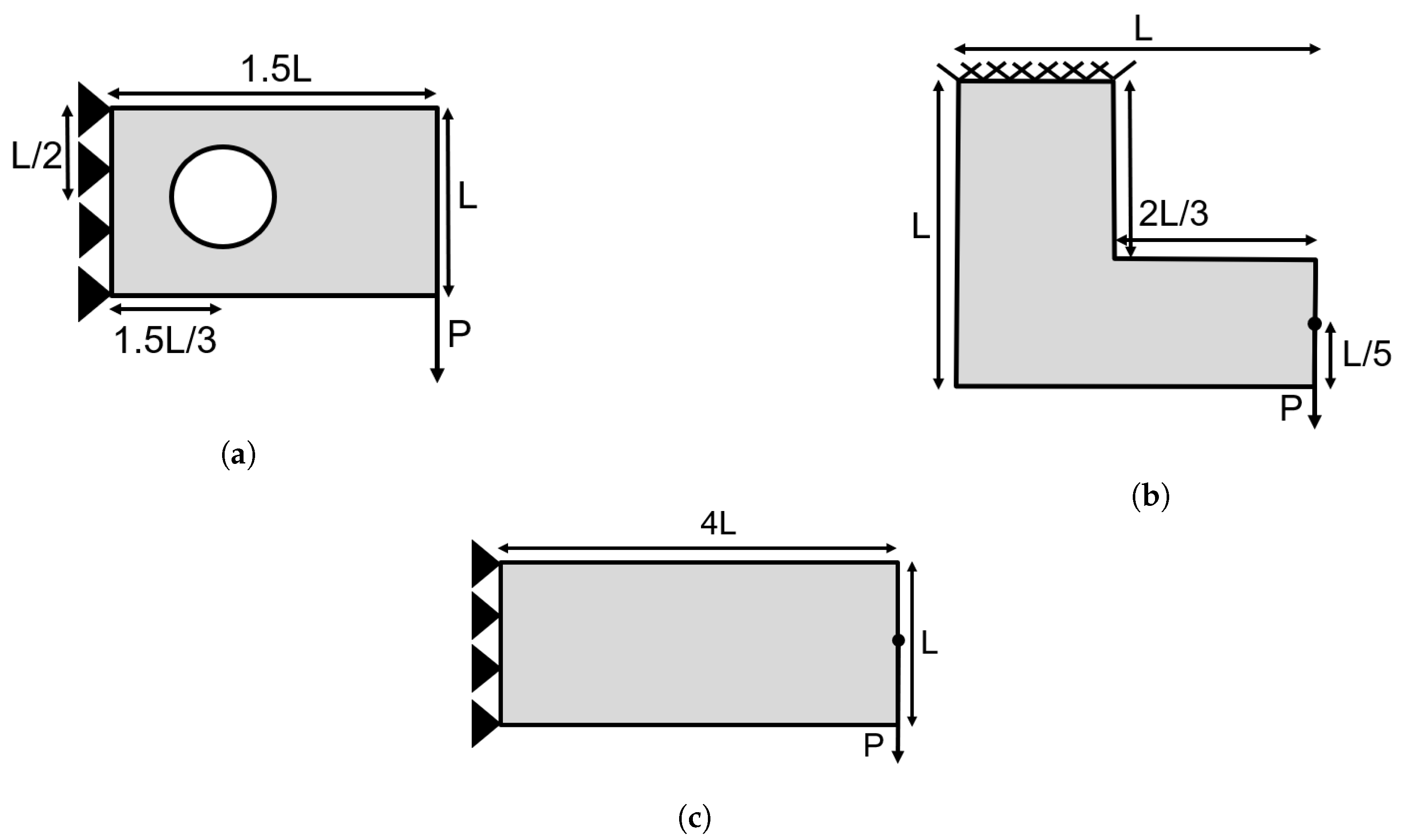
To display the hole at the center of the 3D unit cell, the geometry presented in Figure 1b illustrates only half of the periodic unit cell geometry. Regarding the 2D test cases, three different examples were selected to be optimized. Each of these examples was chosen to illustrate a different application of the methodology. In Figure 2, the design domains along with the loading and boundary conditions for the three test examples are presented.

The first test case presented in Figure 2a refers to a cantilever beam with a hole applied at one-third of its horizontal length and the middle of its vertical length. The second test case presented in Figure 2b refers to the “L shape” geometry with a load applied at its right edge, one-fifth from the bottom. The third test case presented in Figure 2c refers to a long cantilever beam with the load applied at the middle of its left side. In all test cases, the proportions of the horizontal and vertical dimensions are presented in their Figures. For the optimization procedure, the L value was considered equal to 1.

There are two sets of parameters considered for the concurrent multi-scale TO formulation. The first set consists of the geometry parameters, whereas the second set consists of the optimization parameters. In all cases, the periodic unit cell was considered to have square geometry, with a difference in scale of ${10}^{-5}$. The periodic unit cell geometry was discretized with a grid of $50\times 50$ finite elements in the directions of the abscissa and ordinate. Additionally, the loading applied in all test cases denoted as P was equal to 1 and the material was set as an isotropic material with a Young’s modulus E equal to 1 and Poisson’s ratio equal to $0.25$. The applied grid discretizing of each test case was different between them. Hence, the cantilever with a fixed hole test case was discretized with a grid of $150\times 100$ finite elements in the directions of the abscissa and ordinate whereas, the L shape test case was discretized with a grid of $80\times 80$ finite elements in the directions of the abscissa and ordinate. Lastly, the long cantilever test case was discretized with a gird of $160\times 40$ finite elements in the directions of the abscissa and ordinate.

Moving to the second set of parameters, i.e., the optimization parameters, in all test cases a maximum number of optimization iterations was set equal to 200 and an optimization tolerance of $1\%$. Additionally, the penalization factor for the SIMP interpolation scheme was set equal to 3 and the reduction rate for the target volume for the BESO approach was set equal to $5\%$. Regarding the periodic unit cell, a target volume fraction of $50\%$ was considered for all test cases and a sensitivity filtering technique for the BESO-based approach. The filtering radius for the sensitivity filtering was set equal to $1.5$ elements. Regarding the macro domains, different target volume fractions were considered between the test cases, and a sensitivity filtering technique was applied with different filtering radii for each test case. For the cantilever beam with a fixed hole test case, a target volume fraction of $50\%$ and a filter radius of 6 elements were considered. In addition, the long cantilever beam had a target volume fraction of $50\%$ and a filter radius of 3 was considered. 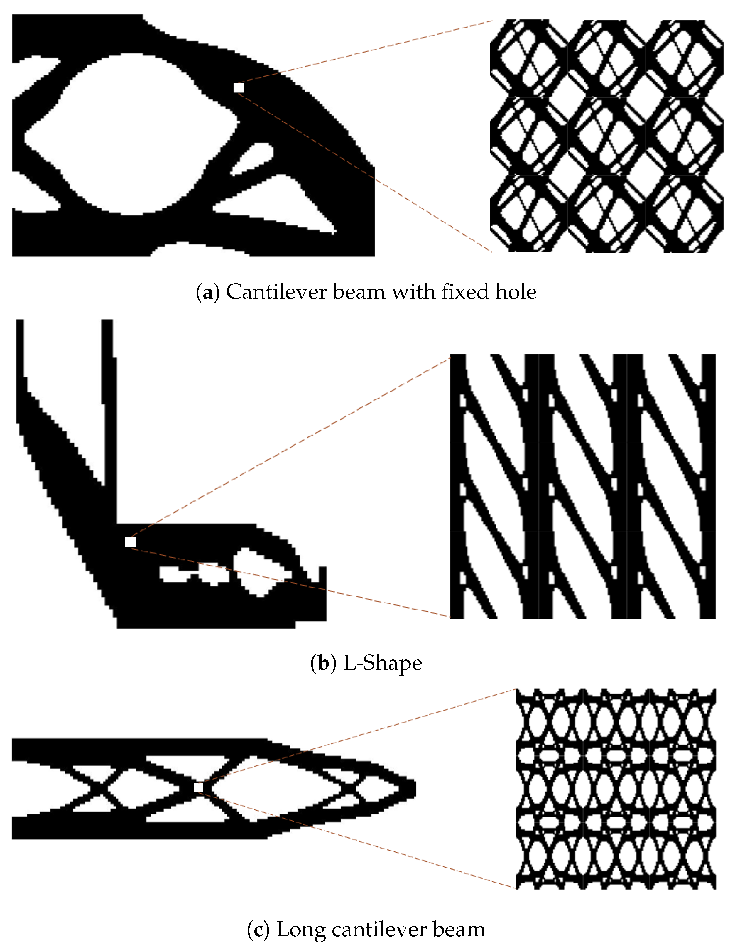Lastly, for the L shape test case, a target volume fraction of $30\%$ and a filter radius of 3 elements were considered. The resulting optimal geometries for both the structural and periodic unit cell are presented in Figure 3.

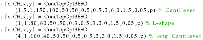
The call to the ConcTopOptBESO function for the three test cases is presented below in Listing 10.

Listing 10 Optimization parameters for the three 2D test cases

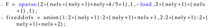
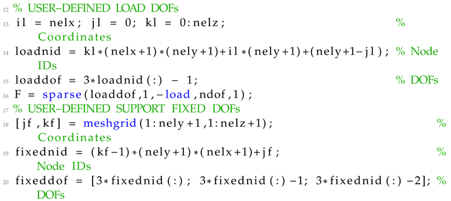
For the implementation of the different support and loading conditions, $Lines$ 15 and 16 are modified depending on the test case. For the cantilever test case, $Lines$ 15 and 16 are modified following Listing 11.

Listing 11 Loading conditions and fixed degrees of freedom for the cantilever test case

For the L-Shape test case, $Lines$ 15 and 16 are modified following Listing 12.

Listing 12 Loading conditions and fixed degrees of freedom for the L-Shape test case

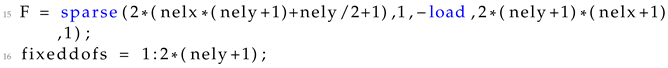
Lastly, for the long cantilever test case, $Lines$ 15 and 16 are modified following Listing 13.

Listing 13 Loading conditions and fixed degrees of freedom for the long cantilever test case

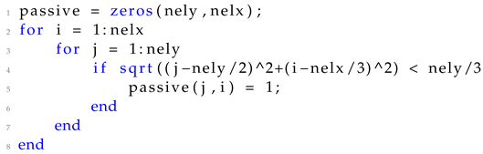
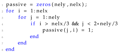
In the implementation of the cantilever beam with fixed hole and L-shape test cases, a set of passive elements is necessary to enforce part of the macro domain to be void. The passive element implementation follows the implementation presented in top88 in [27]. Thus, a matrix called $passive$ is initialized during the initialization step of the optimization procedure following Listing 14 for the Cantilever.

Listing 14 Initialization of the passive element variable for the cantilever test case

and following Listing 15 for the L-shape.

Listing 15 Initialization of the passive element variable for the L-Shape test case

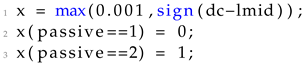
With the matrix $passive$ initialized, two extra $Lines$ are added inside the soft-BESO update scheme of the macro-scale following Listing 16.

Listing 16 Implementation of the passive elements inside the optimization procedure

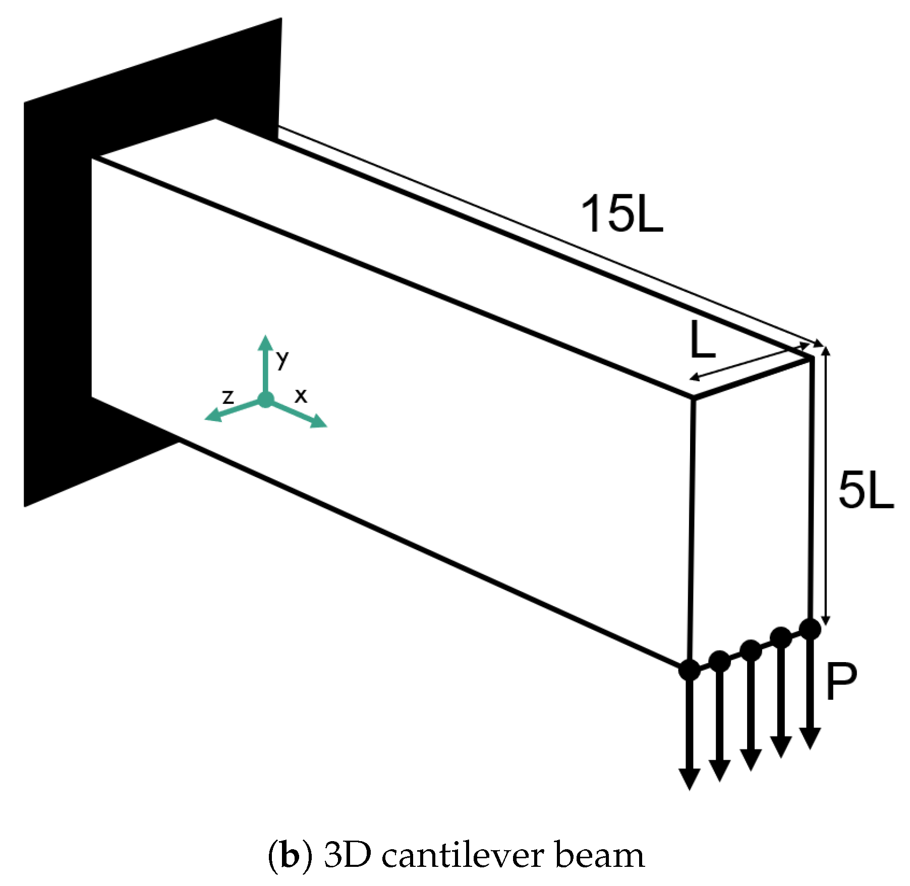
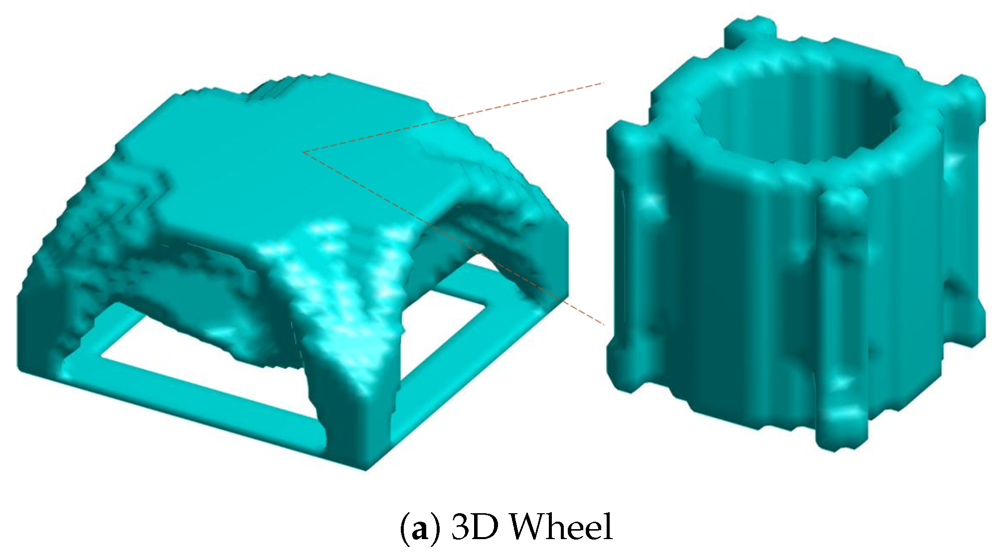
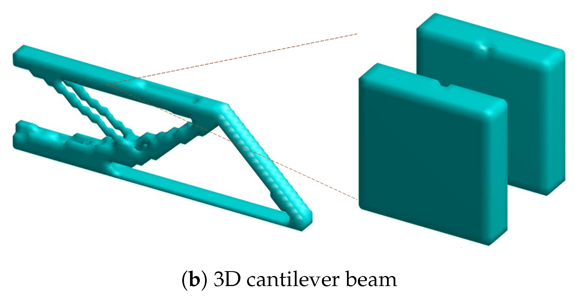
Regarding the 3D test cases, two different examples were selected for optimization. These examples are the 3D cantilever beam and the 3D wheel. A graphic representation of these two test cases is also illustrated in Figure 4.

The first test case presented in Figure 4a refers to the 3D wheel test example, whereas the second test case presented in Figure 4b refers to the 3D cantilever beam. Similarly to the 2D test cases, there are two sets of parameters considered. The first set consists of the geometry parameters and the second set consists of the optimization parameters. Similarly to the 2D test cases, in both test cases, the periodic unit cell was considered to have square geometry, with a difference in scale of ${10}^{-5}$. The periodic unit cell geometry was discretized with a grid of $20\times 20\times 20$ finite elements in the directions of $x,y$ and z, respectively. Furthermore, the loading condition applied to both cases is denoted as P and was set equal to one. The material was set as isotropic with Young’s modulus of one and Poisson’s ratio of 0.25. The discretization of the first test case, i.e., the 3D wheel was set as a grid of $40\times 20\times 40$ finite elements in the directions of $x,y$ and z, respectively. Whereas, the discretization of the second test case, i.e., the 3D Cantilever beam was set as a grid of $60\times 20\times 4$ finite elements in the directions of $x,y$ and z, respectively. The maximum number of optimization iterations was set to 200, with an optimization tolerance of $0.1\%$. The penalization factor for the SIMP implementation was set equal to 3 and the reduction rate for the volume constraint was set equal to $5\%$. The target volume fractions were set equal to $20\%$ and $30\%$ for the 3D wheel and the cantilever test case, respectively. In both cases, a sensitivity filter was applied with an effective radius of $1.5$ elements. The resulting optimal geometries are presented in Figure 5.

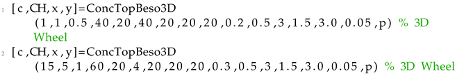
The call to the UCOpt3D for the two 3D test cases is presented in Listing 17.

Listing 17 Optimization parameters for the three 3D test cases

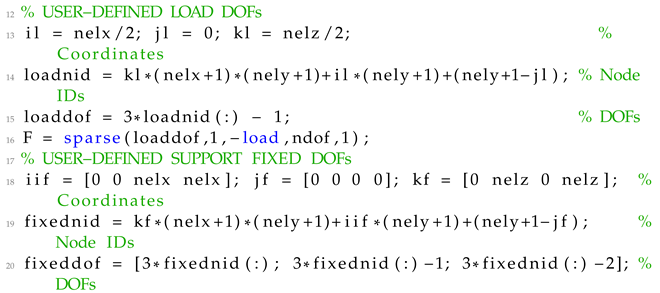
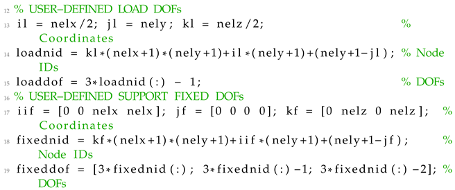
For the implementation of the different support and loading conditions, $Lines$ 12–19 are modified depending on the test case. For the 3D Wheel test case, $Lines$ 12–19 are modified following Listing 18.

Listing 18 Definiton of loading conditions and fixed degrees of freedom for the 3D wheel test case

Whereas, for the 3D cantilever test case, $Lines$ 12–19 are modified following Listing 19.

Listing 19 Definiton of loading conditions and fixed degrees of freedom for the 3D cantilever test case

7. Code Extensions

This section introduces the expansion of the MATLAB implementation discussed in Section 5 to accommodate two-phase composite microstructures. Additionally, it includes additional numerical tests to those presented in Section 6 that are compared to results obtained from existing literature for assessment purposes.

7.1. Two-Phase Composites

In this sub-section, the extension of the two MATLAB codes for two-phase composite microstructures is presented, along with the modification of the volume constraint applied for the micro-scale to accommodate the two different materials. The integration of the two different volume constraints into a single optimization constraint. The single volume constraint is designed to enable the optimization algorithm to allocate the allowed volume fraction target value between the micro and macro-scales. The extension for the use of two-phase composite microstructures in the code implementations is relatively straightforward through the use of the modified SIMP approach. Thus, in Equation (7) the second material can be simulated by replacing the term $E_{min}$ with the Young’s modulus of the second material denoted as $E_2$. Thus, if additionally term $E^0$ is denoted as $E_1$ representing the Young’s modulus of the first material, the expression of Equation (7) is modified into the Equation (22).

$$E_{el}\left(y\right)=E_2+y_{el}^p·(E_1-E_2)$$

(22)

Thus, for elements with $y_{el}$ equal to one their Young’s modulus is equal to, $E_1$ whereas for elements with $y_{el}$ equal to zero their Young’s modulus is equal to $E_2$. Another popular implementation includes the modification of Equation (22) to a more straightforward expression following Equation (23).

$$E_{el}\left(y\right)=y_{el}·E_1+(1-y_{el})·E_2$$

(23)

where the sensitivity of the term $E_{el}$ is following the expression of Equation (24).

$$\frac{\partial E}{\partial y_{el}}=E_1-E_2$$

(24)

The modification of the volume constraint for the micro-scale is based on the constraint presented by Yan et al. in [24]. Thus, in order to balance the two phases, the new volume constraint in addition to the material densities y takes into consideration the difference in density between the two phases. Therefore, the term $V\left(y\right)$ of the volume constraint presented in multi-scale problem formulation (1) is modified following the expression of Equation (25).

$$V\left(y\right)=\sum _{el}^{n_{el}}(y_{el}+(1-y_{el})\ast \frac{{\rho }_1}{{\rho }_2})$$

(25)

where terms ${\rho }_1$ and ${\rho }_2$ refer to the densities of phases one and two, respectively.

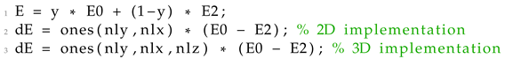
The implementation of the two-phase composite microstructures into the two MATLAB codes requires small changes. For the integration of the second Young’s modulus, if the modified SIMP expression is not replaced with Equation (23), then the only change in both codes is the introduction of the variable $E2$ which replaces variable $E_{min}$. If the modified SIMP expression is replaced with Equation (23), then $Lines$ 85 and 113 of the 2D and 3D codes, respectively, are replaced with the following $Lnes$ presented in Listing 20.

Listing 20 Modified expressions for the Youg’s modulus for the two-phase composite microstructure

Regarding the modified volume constraint, $Lines$ 121 and 150 of the 2D and 3D codes, respectively, are replaced with the following $Line$ for the 2D presented in Listing 21.

Listing 21 Implementation of the microstructure volume constraint in 2D

And the following $Line$ for the 3D presented in Listing 22.

Listing 22 Implementation of the microstructure volume constraint in 3D

where variable r refers to the ratio of the densities of the two phases.

In the presented code implementations, the target volume fractions for the macro and micro-scale are considered as a parameter of the optimization problem. Using different combinations of these two target volumes can result in different objective function volumes. To find the optimal combination of the two target volumes, the two volume constraints can be combined into a single one, which is then imposed into the optimization procedure. Thus, similarly to the constraint presented in [24], the single volume constraint follows the expression of Equation (26).

$$(V\left(x\right)/V_x)·(V\left(y\right)/V_y)=f$$

(26)

where the term $V\left(y\right)$ follows the expression of Equation (25).

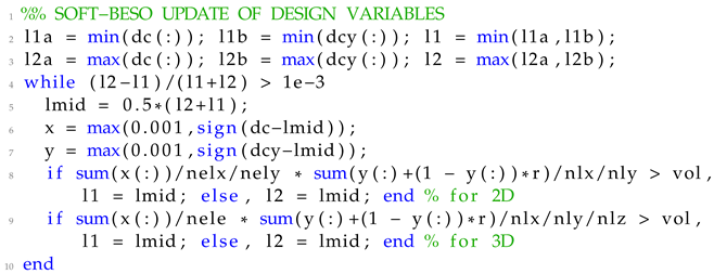
The implementation of the single constraint can be achieved by modifying the BESO update step inside the optimization procedure. Hence, $Lines$ 109–122 and 138–152 of the 2D and 3D implementations, respectively, are replaced with the following update scheme presented in Listing 23.

Listing 23 Implementation of the BESO update scheme for the single volume constraint

7.2. Formulation Comparisons

In this part of the study, two test cases comparing the three different implementations are presented. These implementations include the use of cellular material, composite material, and the single volume constraint. Thus, the following notation is used subsequently for denoting the 3 formulations: Formulation I denoting the multi-scale concurrent formulation with cellular material and two volume constraints; Formulation II denoting the multi-scale concurrent formulation with composite two-phase material and two volume constraints; and Formulation III denoting the multi-scale concurrent formulation with composite two-phase material and a single volume constraint. The first test case considered refers to a cantilever beam, as illustrated in Figure 6.

For this test case, the total volume target for all three implementations was considered equal to $25\%$. This target volume is then divided into $50\%$ for the macro-scale and $50\%$ for the micro-scale. Thus, the volume ratio in the case of the two volume constraints is manually set, whereas for the case of the single constraint, the optimization algorithm will decide it. The parameter setup for the long cantilever test case considered is formulated following Listing 24.

Listing 24 Input parameters for the long cantilver beam test case

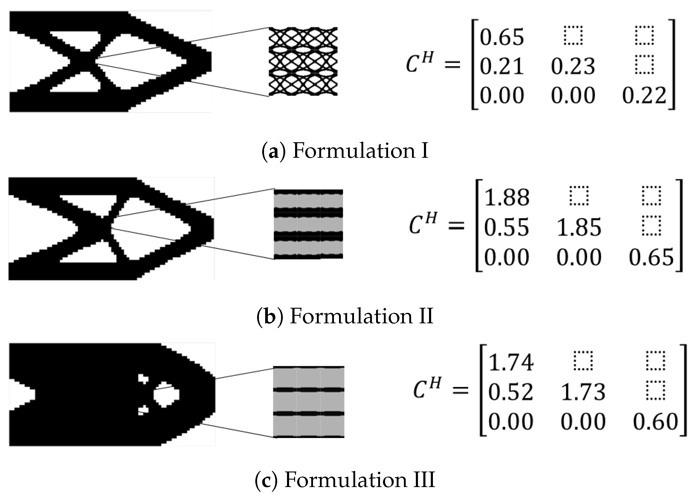
The Young’s modulus considered was set equal to 2 for the main material and $1.5$ for the secondary material, with a Poisson’s ratio of 0.3 for both. In addition, the second material was considered to have a lower by eight times density than the main material. The final geometries as well as the homogenized elasticity tensors for the three different implementations are presented in Figure 7.

In Figure 7a, the optimal geometries for the implementation with the utilization of the cellular material and two volume constraints are presented. In Figure 7b, the optimal geometries for the implementation with composite two-phase material and two volume constraints are presented. Lastly, in Figure 7c, the optimal geometries for the implementation with composite two-phase material and a single volume constraint are presented.

The first implementation, which utilized a cellular material configuration for the micro-scale achieved a relatively (to the other two) high value of the objective function equal to $64.40$. For the second case, where a composite material is utilized but the ratio of volume fraction for the macro and micro-scales was set as an optimization parameter the value of the objective function was lower, equal to 18.30. In the third case, the optimal ratio of the volume fractions between the two scales resulted as equal to $85.6\%$ and $29\%$ for the macro and micro-scale, respectively. For this combination of volume fractions, the value of the objective function achieved was the lowest of all three equal to $13.10$.

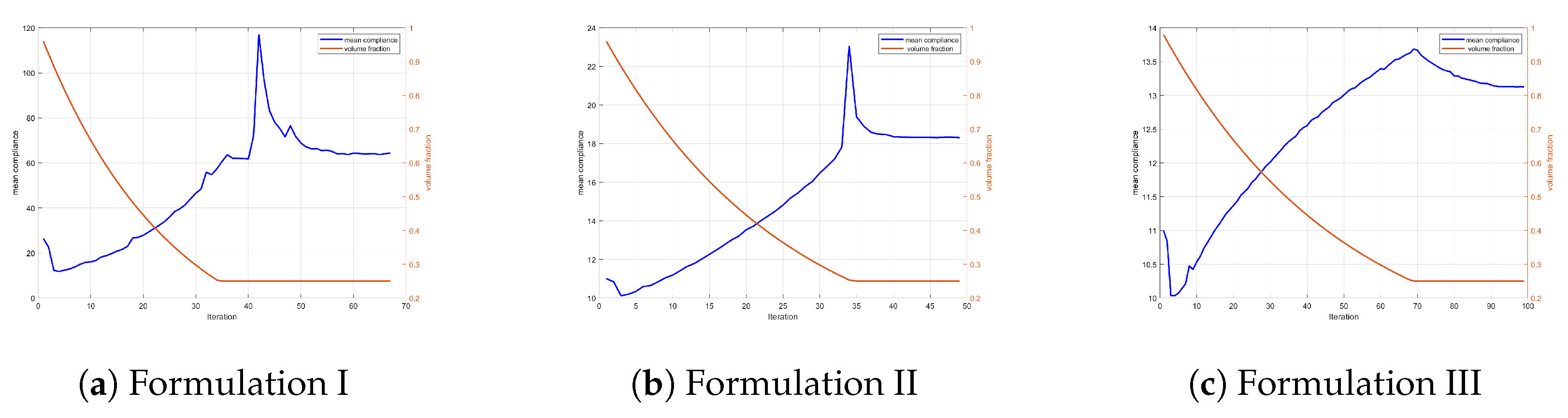
In Figure 8, the evolution histories of the three different formulations are presented. The figures display the total volume fraction, which is calculated as the product of the volume fractions in the macro and micro domains. As depicted in these figures, the third formulation exhibits a smoother transition in the objective function as it approaches the optimization target of a $25\%$ volume fraction.

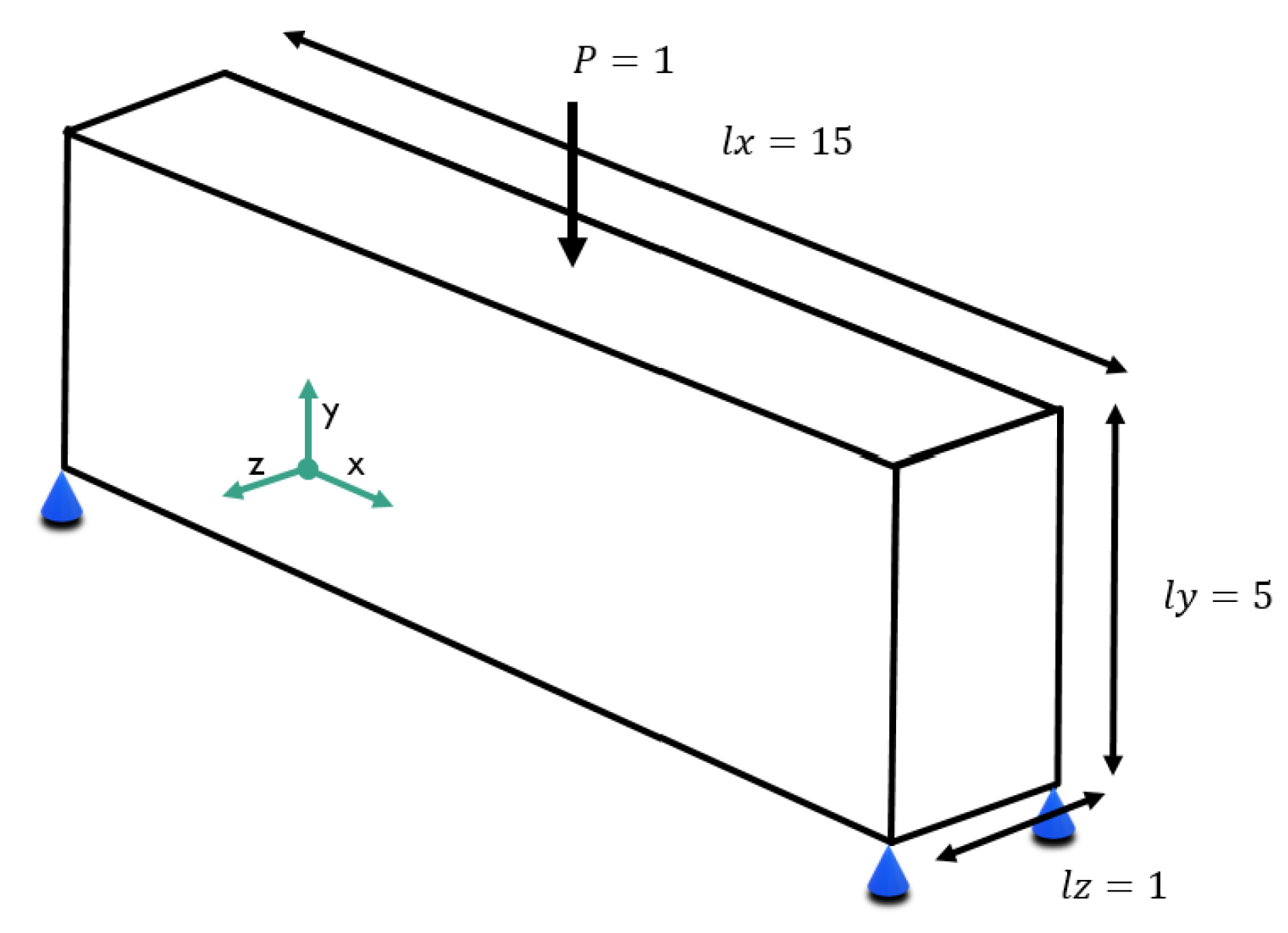
The second test case considered refers to a 3D MBB beam example, as illustrated in Figure 9.

For this test case, the total volume target for all three implementations was considered equal to $30\%$. For the formulation with two volume constraints, the total $30\%$ is set as $50\%$ for the macro-scale and $60\%$ for the micro-scale. In addition, the input parameters for the 3D MBB beam test case are formulated following Listing 25.

Listing 25 Input parameters for the 3D MBB beam test case

Similarly to the 3D test cases presented in the previous section, the boundary and loading conditions are provided by replacing the $Lines$ 12–19 in the UCOpt3D function following Listing 26.

Listing 26 Implementation of the loading conditions and fixed degrees of freedom in the 3D MBB beam test case

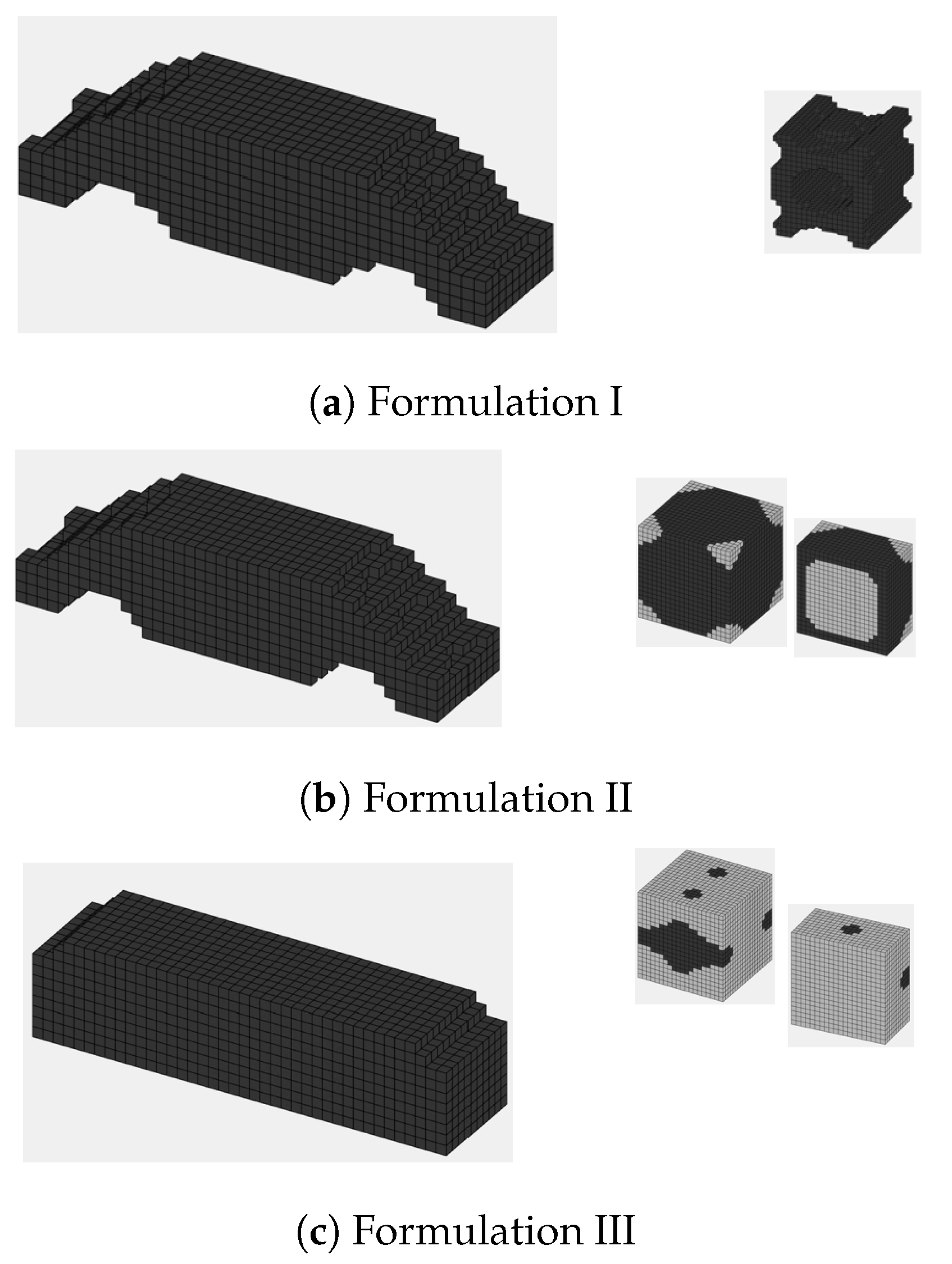
Similarly to the 2D test case, the Young’s modulus for the main material was set equal to 2, and for the secondary material, equal to $1.5$, and the Poisson ratio was equal to 0.3 for both materials. The resulting optimal geometries for both the macro and micro-scales are presented in Figure 10.

In Figure 10b,c, both the unit cell and half of the unit cell are presented, both better understanding of the final geometry. The first implementation presented in Figure 10a managed to achieve an objective function value of $36.57$ whereas the second implementation presented in Figure 10b achieved an objective function value of $11.38$. The third implementation presented in Figure 10c as expected achieved the lower value of the objective function equal to $10.04$. The optimal volume fraction achieved from the third implementation is $94.2\%$ for the macro-scale and $31.8\%$ for the micro-scale.

8. Conclusions

The primary objective of this study was to present a straightforward and efficient implementation of the concurrent multi-scale topology optimization (TO) formulation using the BESO method. By optimizing both the micro and macro-scales concurrently, the implementation ensures optimal topologies without the need for additional black-and-white filtering techniques commonly required in SIMP-based implementations. In our approach, the soft-BESO technique is employed in both the micro and macro-scales, allowing for smooth and continuous transitions in the resulting optimal topologies. This eliminates the issue of checkerboard patterns that can arise in certain TO implementations. As a result, the obtained optimal designs exhibit clear and well-defined structures, represented in black and white. The versatility of our implementation is demonstrated through a range of test cases conducted in both 2D and 3D spaces. These test cases illustrate the implementation’s capability to handle different structural configurations and complexities, showcasing its potential across various practical applications. To further enhance and refine our implementation, we welcome feedback and suggestions from the research community. Interested parties may direct their inquiries or suggestions to the corresponding author via email at [email protected]. Collaborative efforts and constructive feedback will help advance the field of concurrent multi-scale topology optimization and pave the way for improved applications in engineering design and beyond. Furthermore, this work includes the provision of the MATLAB implementation for the proposed methodology. The code will be made available for better understanding and reproducibility of the results. Additionally, a comparative investigation is carried out to assess the performance of the proposed methodology in comparison to existing literature. This allows for a comprehensive evaluation of its effectiveness and highlights any potential improvements or advantages it may offer.

Our research results hold potential for various practical applications, which encompass (i) Engineering Design, (ii) Material Design, and (iii) Multi-Functional Materials. The findings from our study show promise for real-world engineering and material design endeavors, offering advantages in terms of concurrent optimization and material flexibility. However, it is essential to acknowledge that these benefits are accompanied by computational costs and implementation complexities that require careful consideration in practical applications. Looking ahead, future research and collaborative efforts could focus on addressing these limitations to enhance the usability and applicability of our proposed methodology. By tackling these challenges, we can further expand the scope and impact of our research, leading to more efficient and effective solutions for a broader range of engineering and material design applications. The complete MATLAB code for both the 2D and 3D implementations is provided in the GitHub repository listed in https://github.com/nikoslagaros/TOPcodes (accessed on 17 September 2023) here.