The Impact of Additive Manufacturing Constraints and Design Objectives on Structural Topology Optimization

Abstract

To analyze the impact of different objective functions and additive manufacturing (AM) constraints on structural topology optimization, it is necessary to perform an in-depth comparative study. This analysis should consider specific structural design factors, such as compliance, volume, or stress minimization, and assess their effects on the topology optimization for AM. In addition, the inclusion of AM constraints can have a significant influence on various aspects, including optimal part geometry, part volume, support structure volume, and structural performance. Thus, it is essential to investigate and compare these factors to determine the optimal part design for AM. This study focuses on comparing topology optimization results obtained using compliance, stress, or multi-objective minimization, with and without AM constraints. A comparative analysis was conducted in the study, utilizing three structural design examples: cantilever beam, bridge-shaped structure, and L-shaped beam. The comparison results provide insights into the effects of build orientation, AM constraints such as overhang, and different design objectives on the structural topology optimization for AM.

1. Introduction

Additive manufacturing (AM) or 3D printing is recognized as a more favorable alternative to traditional manufacturing methods, especially for applications requiring high structural performance and advanced low-volume production [1]. In particular, incorporating topology optimization into AM allows both technologies to reach their full potential [2]. The objective functions in topology optimization define the design goals, such as minimizing stress and volume, maximizing stiffness, or minimizing compliance (i.e., the inverse of stiffness) of the structure [2,3,4]. In topology optimization, the structural performance is evaluated iteratively under different topologies in order to find the optimal geometry. By incorporating AM constraints and design objectives into the topology optimization process, the final design can be optimized to meet the structural and manufacturing requirements while being feasible, cost-effective, and efficient for AM [3,5,6,7,8]. For example, considering AM constraints such as overhang and member size in the design process is essential to minimize the need for support structures, which are wasteful in terms of material and can increase post-processing costs during manufacturing. Successful design for AM involves optimizing the geometry, material selection, and manufacturing approach to meet these AM constraints and achieve the desired functional performance. When considering overhang and member size, many AM processes deposit material layer by layer, which can lead to problems that extend horizontally without proper support. Overhangs and features with steep angles can cause drooping, sagging, or collapsing during printing. Designers need to consider where and how to add support structures to prevent overhangs from failing. Support structures provide temporary scaffolding that is later removed after printing. In addition, the precision of AM processes can be limited by factors like nozzle size, layer height, and material properties. Small features may be inaccurately printed or fail to form properly. Designers should adhere to minimum feature sizes, understand the resolution limitations of the chosen AM technology, and avoid designing features that are smaller than what the process can accurately reproduce [9,10,11,12].

Topology optimization that incorporates AM constraints and builds orientation enables the optimization of part designs that not only meet structural requirements but also take into account the limitations and capabilities of AM processes. By considering the build direction, the optimization process ensures that the design can be manufactured with minimal support structures and reduces the need for additional post-processing steps [13]. Several studies have been conducted to topologically optimize designs using AM constraints to reduce the need for post-processing [9,14,15]. To impose layer-wise overhang constraints and achieve specific overhang thresholds of 45 degrees, voxel-based topology optimization frameworks were employed [15]. An image-based computational approach was utilized to control the optimized maximum or minimum lengths within the design [16]. Furthermore, optimization techniques such as combining compliance and overhang as objectives, applying overhang constraints with hanging features, and setting arbitrary thresholds based on voxel aspect ratios have been adopted, and the modified moving asymptotes process and the bi-directional evolutionary structural optimization (BESO) approaches have also been utilized in the literature [15,16,17,18]. The use of ANSYS APDL to reduce compliance and ensure the absence of overhanging surfaces also showed the impact of incorporating AM constraints [19,20].

Despite the significant progress in the field of design for AM, there is a lack of comprehensive studies that investigate the impact of AM constraints and different design objectives on topology optimization for AM. This study aims to fill this gap by analyzing the effects of AM constraints, such as overhang and member size, and different design objectives (e.g., compliance, stress, or multi-objectives) on structural topology optimization. It also focuses on providing a deeper understanding of how to formulate design problems for AM and to balance the trade-offs between design objectives, total volume, and manufacturing feasibility with respect to support structures.

2. Methods

2.1. Topology Optimization

In the general formulation for topology optimization, the design variables are assigned to each element in the mesh and are denoted as ${\eta }_i$, a pseudo-density ranging from 0 to 1. A value of 0 indicates that the material should be removed, while a value of 1 indicates that it should be retained. The goal of the optimization process is to find the optimal values of these design variables to achieve the desired objective [21].

The mathematical formulation for topology optimization can be represented as:

$$\mathrm{Maximize}\mathrm{or}\mathrm{minimize}f({\eta }_i)$$

(1)

$$\mathrm{subject}\mathrm{to}0<{\eta }_i\le 1\hspace{1em}\hspace{1em}(i=1,2,3\dots ,m)$$

(2)

$$g_j\le g_j^{\max }\hspace{1em}\hspace{1em}(j=1,2,3\dots ,n)$$

(3)

Here, m and n are the number of finite elements and the number of constraints, respectively, and $g_j^{\max }$ is the upper limit for the constraint $g_j$.

2.1.1. Density-Based Approach

The density-based approach involves using constant material properties in each element of the discretized design domain. The formulation of this approach was developed based on the pioneering work on homogenization methods [22].

This approach depends on the Young’s modulus $\left(E_e\right)$ and the relative density $\left(x_e\right)$ of the element and is represented as:

$$E_e\left(x_e\right)={\left(x_e\right)}^{p}E\hspace{1em}0<x_{\min }\le x_e\le 1$$

(4)

where

• p: Penalization factor greater than 1 (e.g., 1.5 < p < 7)
• E: Young’s modulus in the base material
• $x_{\min }$: Minimum value of the relative density

When Young’s modulus of a void material is assigned, the modified Solid Isotropic Material with Penalization (SIMP) method uses non-zero values to avoid the singularity in the finite element stiffness matrix.

$$E_e\left(x_e\right)=E_{\min }+{\left(x_e\right)}^p(E_0-E_{\min })\hspace{1em}{x}_e\in [0,1]$$

(5)

where $E_{\min }$ is a very small stiffness, and $E_0$ is the stiffness of the material [22].

To solve nonlinear programming problems for minimizing stress, compliance, volume, etc., the method of moving asymptotes (MMA), sequential quadratic programming (SQP), or optimality criteria methods have been used in the literature. The optimality criteria method utilizes the Karush-Kuhn-Tucker (KKT) condition to determine the optimal solution [23]. The termination criteria for the optimization process are either reached when the maximum number of iterations is reached without meeting the optimal criteria or when the convergence termination criteria are satisfied. One of the convergence criteria is based on the difference between the new and old values of the design variables (i.e., $|{\mathbf{x}}^{\mathrm{new}}-{\mathbf{x}}^{\mathrm{old}}|$). If the difference between these two design variable values is smaller than the tolerance, the topology optimization process is terminated.

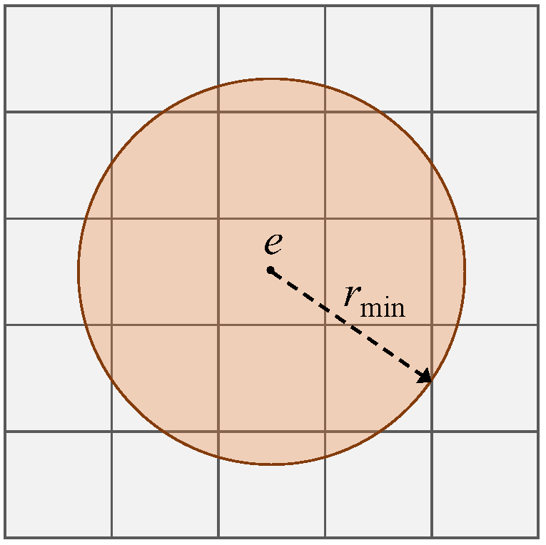
2.1.2. Filter Function

One issue that can arise in topology optimization is the presence of “checkerboard effects”, which are patterns of alternating solid and void elements arranged in a checkerboard-like fashion. These checkerboard patterns can lead to problems such as buckling with zero performance [24].

The basic density filter calculates a new relative density for elements based on the neighborhood. This is achieved by summing the relative densities $x_f$ of the elements in the neighborhood $N_e$ of a given element $x_e$ and dividing this sum by the total volume $V_f$ of these elements. The neighborhood $N_e$ of an element $x_e$ is defined as the set of elements $f$ that are within a certain distance $d\left(e,f\right)$ from the element $x_e$. It can be visually represented, as seen in Figure 1.

Mathematically,

$$x_e=\frac{{\displaystyle \sum _{f=1}^{N_e}{H}_{ef}{V}_f{x}_f}}{{\displaystyle \sum _{f=1}^{N_e}{H}_{ef}{V}_f}}$$

(6)

where $N_e=\{f:d(e,f)\le r_{\min }\}$.

In Equation (6), the height factor $H_{\mathrm{ef}}$ is a function of the filter size $r_{\min }$ and the distance between elements $d\left(e,f\right)$. $H_{\mathrm{ef}}$ is calculated as the difference between $r_{\min }$ and $d\left(e,f\right)$ for the elements $f$ in the neighborhood $N_e$.

$$H_{ef}=r_{\min }-d\left(e,f\right)\hspace{1em}\mathrm{where}{f\in N}_e$$

(7)

2.2. Manufacturing Constraints in ANSYS

To enhance the optimization of product design and manufacturing processes, ANSYS provides several types of manufacturing constraints. These constraints, when integrated into ANSYS, enable the optimization of product performance to meet the specific requirements of AM. Two notable types of manufacturing constraints in ANSYS are (1) overhang and (2) member size constraints. The overhang constraints can be applied by defining the maximum allowable overhang angle, typically set at 45 degrees, for a particular part with a given build direction. This constraint ensures that overhanging features within the part do not exceed the defined angle, thereby maintaining structural integrity during the manufacturing process. Additionally, member size constraints can be employed by setting parameters such as minimum thickness or maximum allowable cross-sectional area for a given part [25]. These constraints allow us to control the size and dimensions of structural elements within the design. This approach ensures that the optimization process takes into account the constraints imposed by AM, and it facilitates the creation of well-optimized parts that balance structural integrity and design requirements in AM scenarios.

2.3. Comparative Study

This study focuses on topology optimization for three different shapes: a cantilever beam, a bridge-shaped structure, and an L-shaped beam. For each individual shape, topology optimization is performed under three different objectives (i.e., (i) compliance, (ii) stress, and (iii) stress and compliance minimization) to determine optimal geometries and predict their performance with or without AM constraints (i.e., overhang and member size).

First, the topology optimization problems can be formulated without AM constraints as:

Minimize:

(i) Compliance, (ii) Stress, or (iii) Compliance + Stress

(8)

Subject to:

$$\mathrm{Volume}\mathrm{fraction}\mathrm{constraint}:V\le V_{\max }$$

(9)

where $V_{\max }$ is the maximum allowed volume, which ensures the optimized design does not exceed the ultimate volume limit. Similarly, the problem formulations with AM constraints can be represented as:

Minimize:

(i) Compliance, (ii) Stress, or (iii) Compliance + Stress

(10)

Subject to:

$$\mathrm{Volume}\mathrm{fraction}\mathrm{constraint}:V\le V_{\max }$$

(11)

$$\mathrm{Overhang}\mathrm{constraint}:h\le h_{\max },\alpha \le {\alpha }_{\max }$$

(12)

$$\mathrm{Member}\mathrm{size}\mathrm{constraint}:t_{\min }\le t\le t_{\max }$$

(13)

where, h, $h_{\max }$, α, ${\alpha }_{\max }$ are the overhang size, maximum size, overhang angle, and maximum overhang angle, respectively, while t, t_min, and t_max are the member size, minimum allowable size, and maximum allowable size.

After topology optimization for six different formulations took place, a validation process of the optimal geometries was also performed in ANSYS. Each optimal design is imported into ANSYS Space Claim to assess its manufacturability and then undergoes structural analysis to verify and obtain the equivalent stress on the design.

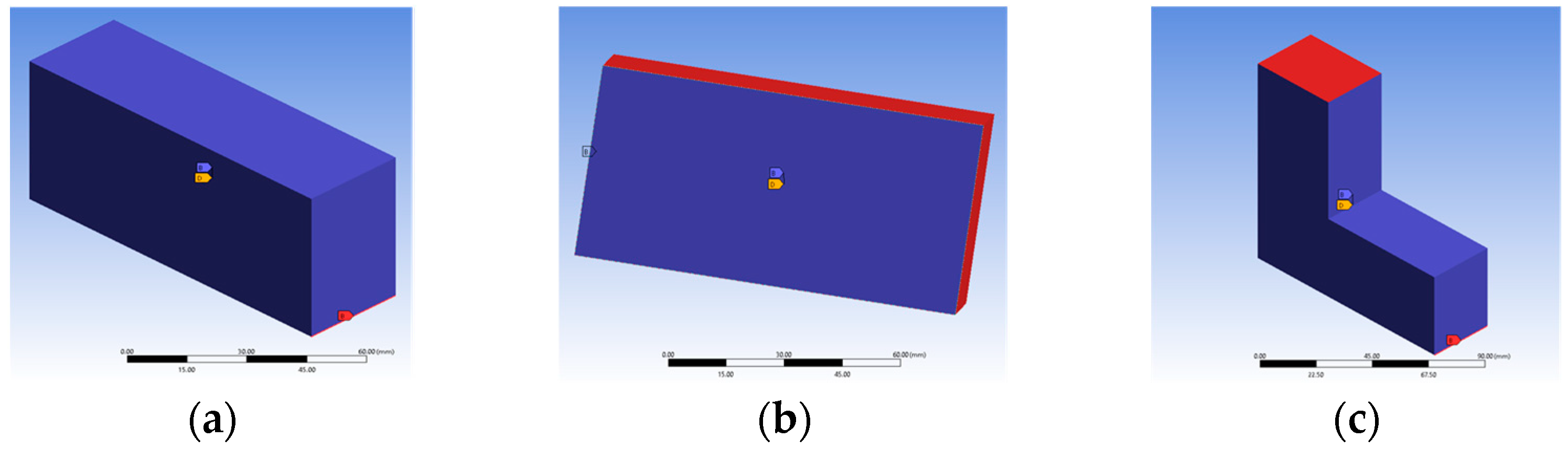
2.3.1. Part Shape and Material

In this work, three conventional designs (i.e., cantilever beam, bridge-shaped structure, and L-shaped beam) are adopted for the comparative study. As seen in Figure 2, the initial dimension of 100 mm × 50 mm × 30 mm is selected for a rectangular profile to be formed into cantilever and bridge shapes. In the figure, the red area indicates the exclusion region that is not considered during optimization, where the purple area indicates the topology or design region, and the yellow arrow indicates the addition of response constraints. The initial design domain of the L-shaped beam has a height and width of 100 mm each. The leg height of 40 mm is defined with a form gap of 60 mm and a thickness of 30 mm. As shown in

Table 1. Material Properties.

Properties	Values
Density	4400 kg/m3.
Melting point	1675 °C
Young’s modulus	114 GPa
Tensile strength	895 MPa
Yield strength	828 MPa
Poisson’s ratio	0.37
Thermal expansion coefficient	8.9 × 10⁻⁶/°C
Specific heat	0.0005 J/kg·°C

, Ti-6Al-4V was selected as the material because it is one of the widely used materials for metal AM in industry. Ti-6Al-4V has a high strength-to-weight ratio and a high modulus of elasticity, which ensures that the designed structure will be stiff and have less deflection. The material property is based on the nonlinear material data available in the ANSYS Workbench Additive Manufacturing Material Library.

Meshing is then performed in the initial stage of structural analysis. A multi-zone meshing method is used. Multi-zone meshing is a meshing technique used in computational modeling and simulation, particularly for complex geometries. It involves dividing the computational domain into separate regions or zones and then creating a mesh for each of these zones independently. It is used because it is advantageous when dealing with models that have areas with different stress levels or different material properties. This method allows the creation of a mesh that is specifically tailored to the behavior of each region, thus increasing the accuracy of the analysis results [26]. For the cantilever beam, a vertical load of 100 N is applied to the lower right area of the opposite free end (Figure 3a). For the bridge-shaped structure, both lateral ends are provided with a fixed support, and a uniformly distributed load of 100 N is applied to the top (Figure 3b). In the L-shaped beam, the upper part of the larger section is fixed while the right bottom edge of the lower end is assigned the load of 100 N (Figure 3c). Next, the solver option is used to perform the structural analysis in ANSYS.

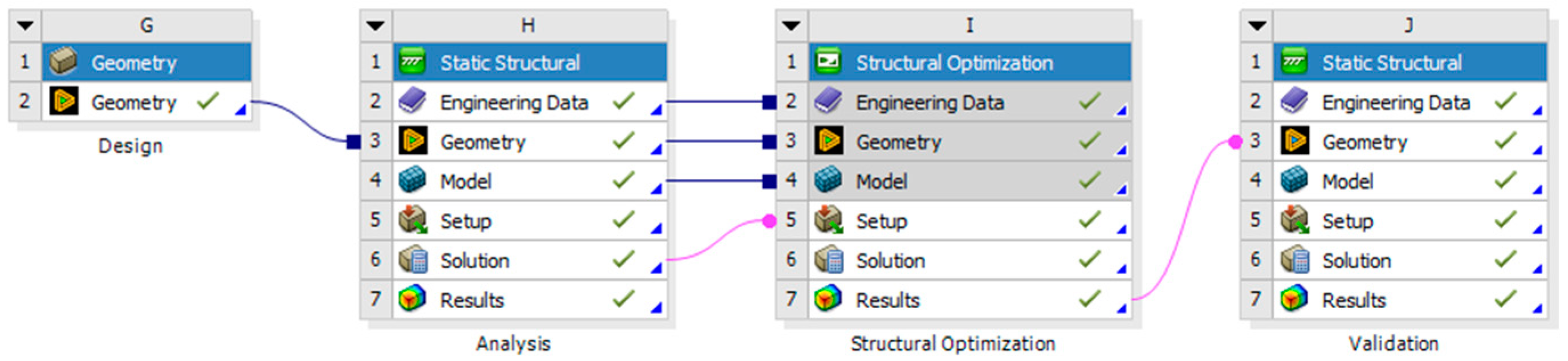
2.3.2. Topology Optimization in Ansys

• Topology Optimization without AM Constraints:

In Phase 1, the objective functions (i.e., compliance, stress, and stress and compliance) and the volume constraint were only used to find the optimal geometry. In the first phase of optimization, the variables of compliance and stress are minimized both together and individually relative to the volume fraction constraint (i.e., $V\le V_{\max }$). In this study, $V_{\max }$ is set to be 30% of the initial design domain volume.

• Topology Optimization with AM Constraints:

In the second phase, the AM constraints (overhang and member size) are employed along with the volume constraint to perform the topology optimization. In order to use the overhang constraint, the build orientation is set in ANSYS. The build orientation may have a significant impact on the final optimized design, so in the presence of overhang constraints, topology optimization is performed for all three cases to study orientation effects. Six different build orientations (±X, ±Y, and ±Z) are selected for additive manufacturing, and the best build orientation with the lowest objective function value is also used for further analysis in Section 3.2 and Section 3.3. As part of the final analysis, three types of objective functions with volume and AM constraints are defined for topology optimization. Compliance, Stress, or Compliance + Stress is minimized subject to the volume fraction constraint and AM constraints, including (1) overhang (the maximum allowable overhang angle = 45°) and member size (the minimum member size = 25 mm).

2.4. Design Validation and Post-Processing

After performing topology optimization in both cases, the optimized geometry is then transferred to ANSYS Space Claim for design validation, as shown in Figure 4. This process is performed to remove all rough surfaces and smooth the faced geometry before sending it to the 3D printer for further operations. It is an intermediate step that is also used as a method of validating the design used in this study. The original face “transfer to design validation” option is used to link the optimized facet data to Space Claim and smoothed for further analysis. After refining the designs, structural analysis is performed again on these features, and the maximum equivalent stress is obtained. Finally, the obtained stress is compared to the ultimate limit of the material to verify the safety and feasibility of the design.

2.5. Support Volume Calculation

In order to compare the support structure volume depending on part geometry, it is necessary to calculate the support volume from a topologically optimized design. In this work, the STL file obtained from ANSYS is read in MATLAB using the pre-written STLREAD code [27], and the support structure volume is calculated in MATLAB. The support volume code uses computational geometric data, such as calculating the minimum and maximum values of the X, Y, and Z coordinates of a set of vertices to determine the bounding box of a 3D object.

Given a set of vertices in 3D space, the minimum and maximum values of the X, Y, and Z coordinates can be calculated as follows:

$$X_{\min }=\min (v(:,1)),Y_{\min }=\min (v(:,2)),Z_{\min }=\min (v(:,3))$$

(14)

$$X_{\max }=\max (v(:,1)),Y_{\max }=\max (v(:,2)),Z_{\max }=\max (v(:,3))$$

(15)

where v(:,1), v(:,2), and v(:,3) are the X, Y, and Z coordinates of the vertices, respectively. The computation of the geometric data involves determining the volume of a rectangular parallelepiped. This volume can be calculated as:

V = (Z_max − Z_min) × (Y_max − Y_min) × (X_max − X_min)

(16)

The code utilizes the matrix representation of vertices and the manipulation of matrices to extract the X, Y, and Z coordinates of the vertices associated with support structures. The matrix representation of a set of vertices in 3D space can be represented as follows:

$$\mathbf{v}=\{v_1,v_2,\dots ,v_{\mathrm{nv}}\}$$

(17)

3. Results and Discussion

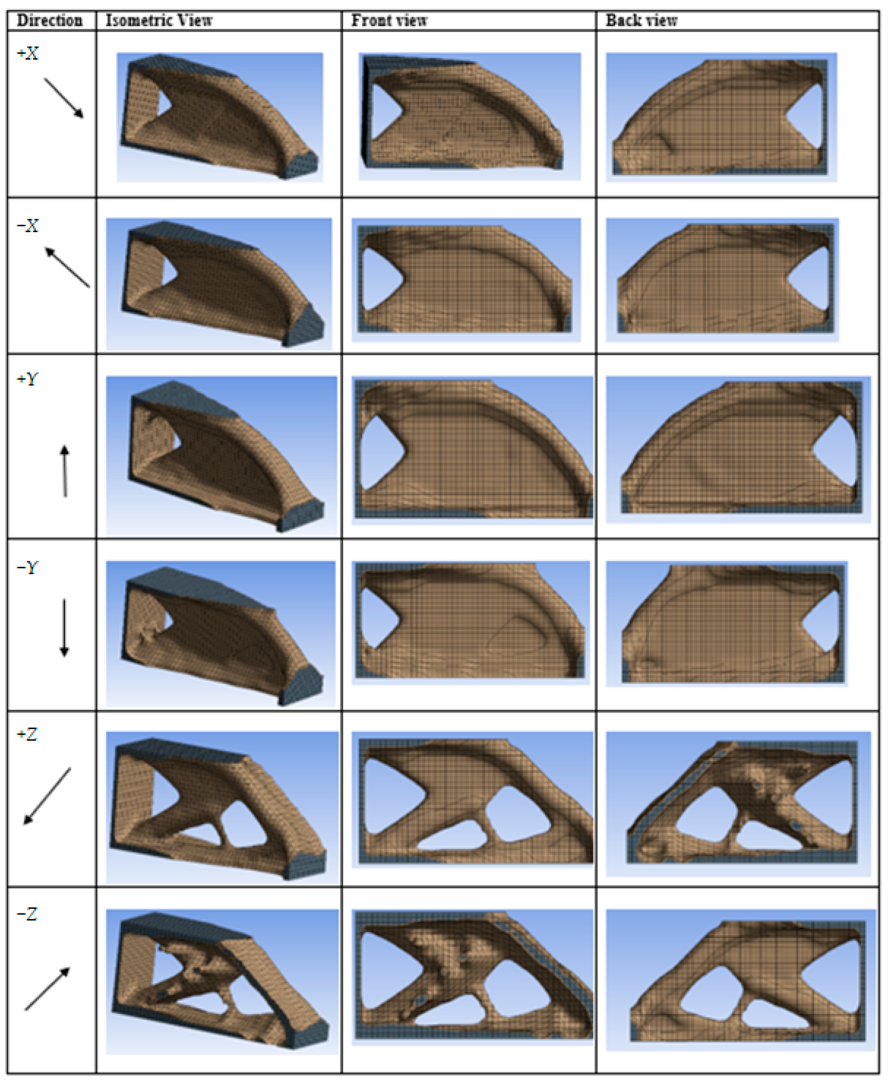
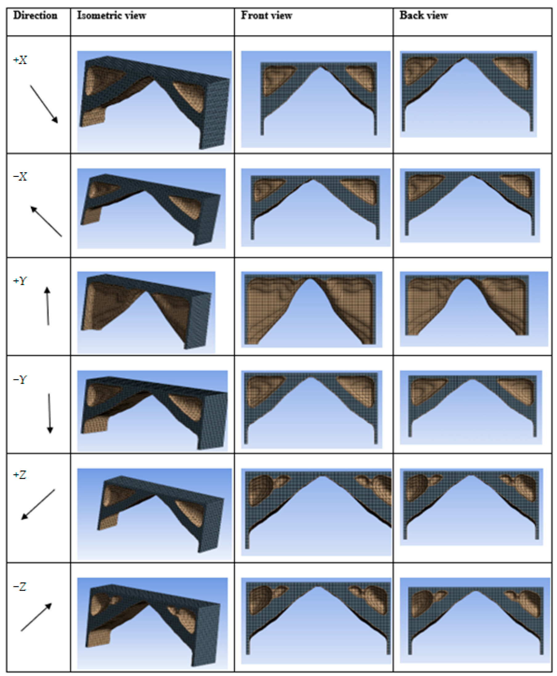
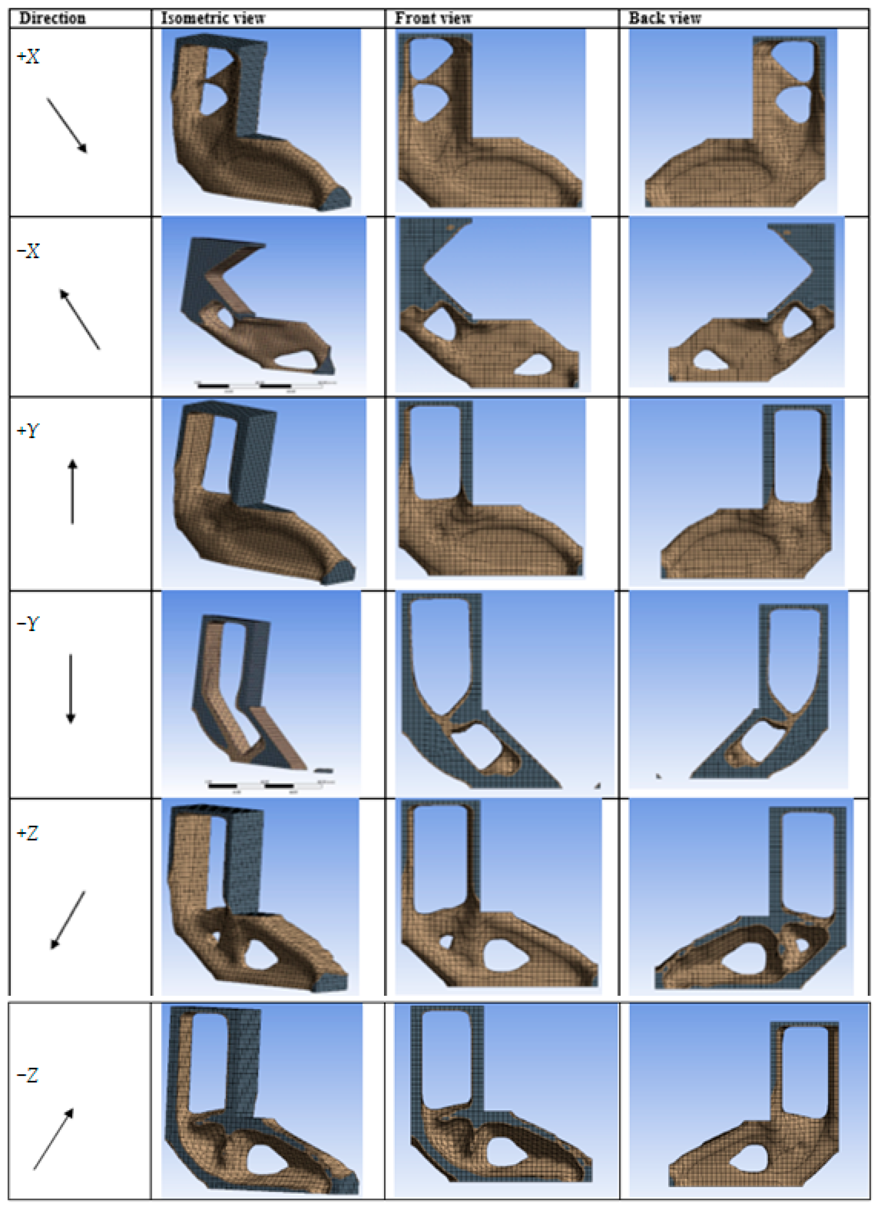
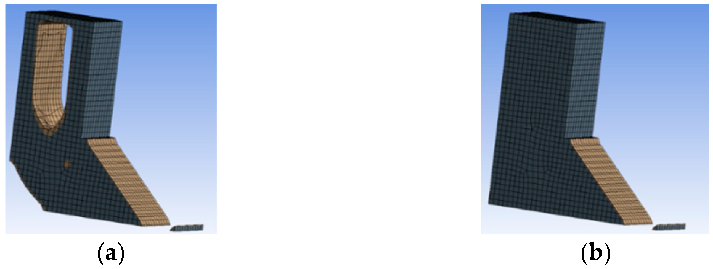
3.1. Build Orientation Effect

The effect of the build orientation on optimal part geometries and objective functions is presented for three case studies: cantilever, bridge shape, and L-beam. The topology optimization with AM constraints such as overhang is performed to minimize compliance under six different build orientations. The optimization results are shown in

Table 2. Results of compliance minimization in six different build orientations.

Build Orientation	Cantilever Beam	Bridge Shape	L-Shaped Beam
+Z axis	0.2147	0.003717	0.5392
−Z axis	0.2473	0.003710	0.5391
+X axis	0.1855	0.003714	0.5388
−X axis	0.1808	0.003710	2.6580
+Y axis	0.1861	0.003367	0.4863
−Y axis	0.1857	0.003680	-

and Figure 5, Figure 6 and Figure 7. In the case of the cantilever example, the minimum compliance was achieved when the build orientation was along the −X direction. Similarly, for the bridge-shaped design and the L-beam, the +Y direction yielded the best results with the smallest values for the design objective. Interestingly, the impact of build orientation on the optimal geometry is relatively smaller for the bridge shape compared to the cantilever and L-shaped beams. This result shows that the bridge geometry is less sensitive to variations in build orientation due to the overall symmetric geometry and load distribution characteristics of the bridge example. However, for the cantilever, when the build orientation is in the ±Z directions, the optimizer attempted to reduce the support structures (i.e., surface angles greater than 45°) but resulted in non-symmetric geometries and uneven surfaces, as shown in Figure 5. These converged results are not ideal and would require significant post-processing time and cost to correct. On the other hand, when the build orientation is in the ±X and ±Y directions for the cantilever example, the optimizer converges to overly simplified shapes to reduce support structures. This is because the optimization process with these build orientations prioritizes minimizing support structures over exploring intricate designs to reduce part volume. Additionally, in the case of the L-shaped beam, when the build orientation was along the −X and −Y directions, the optimized design was redundant, and convergence could not be achieved, while non-symmetric geometries were observed when the build orientation was in the ±Z directions. It is likely that the results are due to the inherent geometry of the L-shape, which does not align well with these orientations.

These results show that selecting the appropriate build orientation is critical and depends on the specific part geometries. Improper build orientation can lead to suboptimal designs, non-symmetric geometries, and difficulties in achieving convergence during topology optimization. It is essential to carefully consider the build orientation to ensure that topology optimization is effectively applied in AM processes.

3.1.1. Case 1: Adjusting the Volume Constraint

The impact of build orientation on optimal geometry is significant, but other factors, such as volume fraction, loading conditions, and material properties, are sometimes overlooked. To comprehensively evaluate the effect of build orientation, the influence of volume fraction and boundary conditions was investigated using two L-shaped designs built in the −X and −Y directions. These specific designs were selected because they exhibited the highest deviation in target and convergence error, respectively.

To investigate the cause of the structural redundancy observed in the L-shaped beam when built in the −X and −Y directions, a reanalysis was performed by adjusting the volume constraints. Specifically, the overhang constraint remained constant for both directions, while the volume fraction was changed from 30% to (1) 50% and (2) 80% to examine the convergence process. The analysis revealed that when analyzing the −Y direction, attempts to achieve an optimal structure were unsuccessful due to persistent redundancy, as shown in Figure 8. This redundancy may have occurred because the outer portion of the leg did not fall within the convergence limit of the overhang with an angle greater than or equal to 45 degrees during the part build along the −Y direction. In the −X build direction for the L-shaped design, increasing the volume fraction to 50% and 80% also led to a similar result.

3.1.2. Case 2: Adjusting the Loading Condition

The loading condition of the L-beam was changed from the lower right corner of the leg to the right face, while all other factors remained unchanged, as shown in Figure 9a. The result of the topology optimization shows that there is no significant improvement in the structure of the beam despite a substantial increase in the objective function values. Moreover, the optimized design has limited practical applicability and would require more post-processing efforts as seen in Figure 9b,c.

Using various computational experiments with different build orientations, it has been observed that even when changing constraint combinations or loading conditions, there remains a potential for challenges in manufacturability within the optimized design. It is possible that the design may require extensive post-processing efforts after topology optimization. Therefore, the selection of the appropriate build orientation becomes crucial in topology optimization, especially when incorporating overhang constraints.

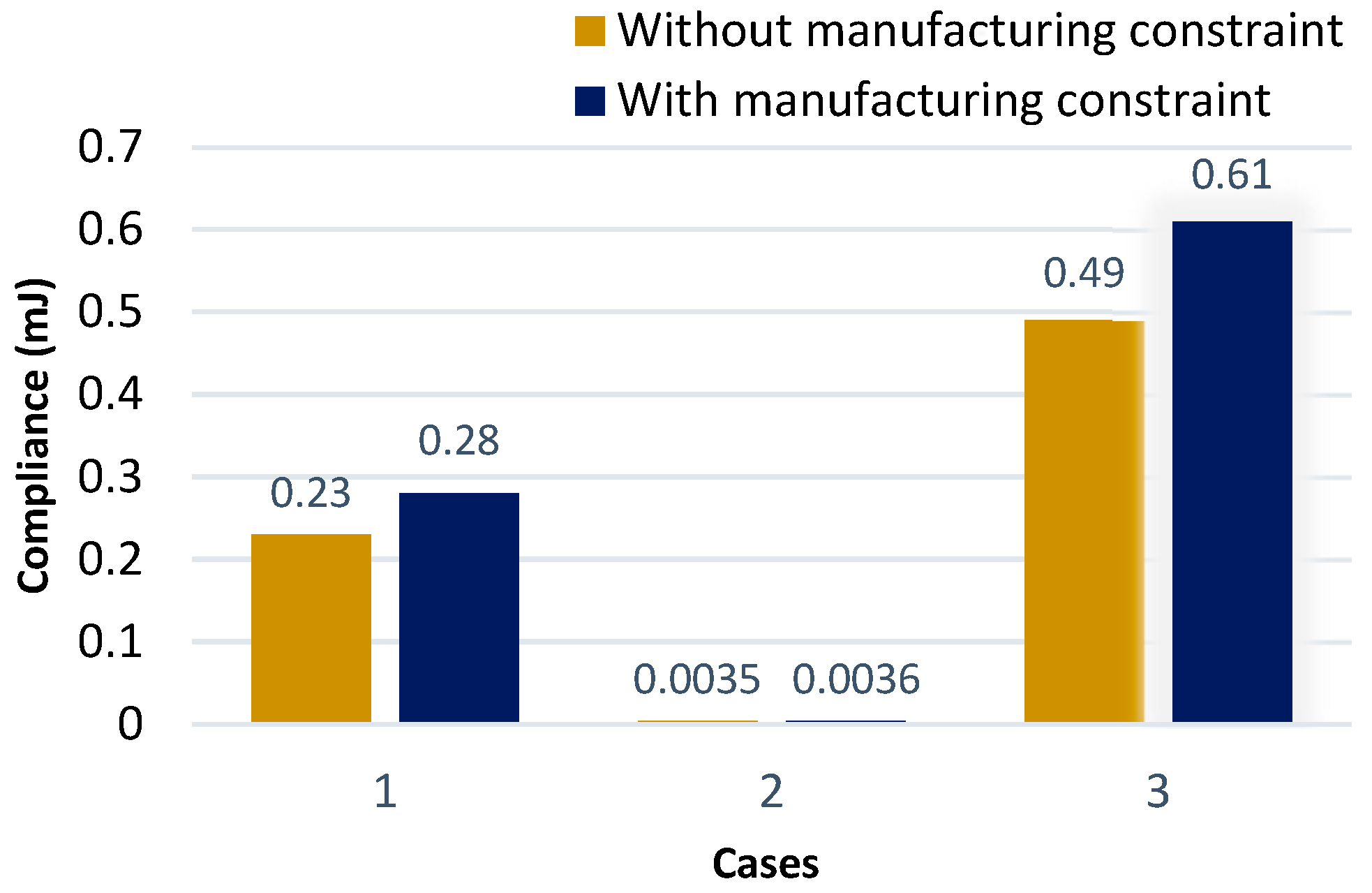
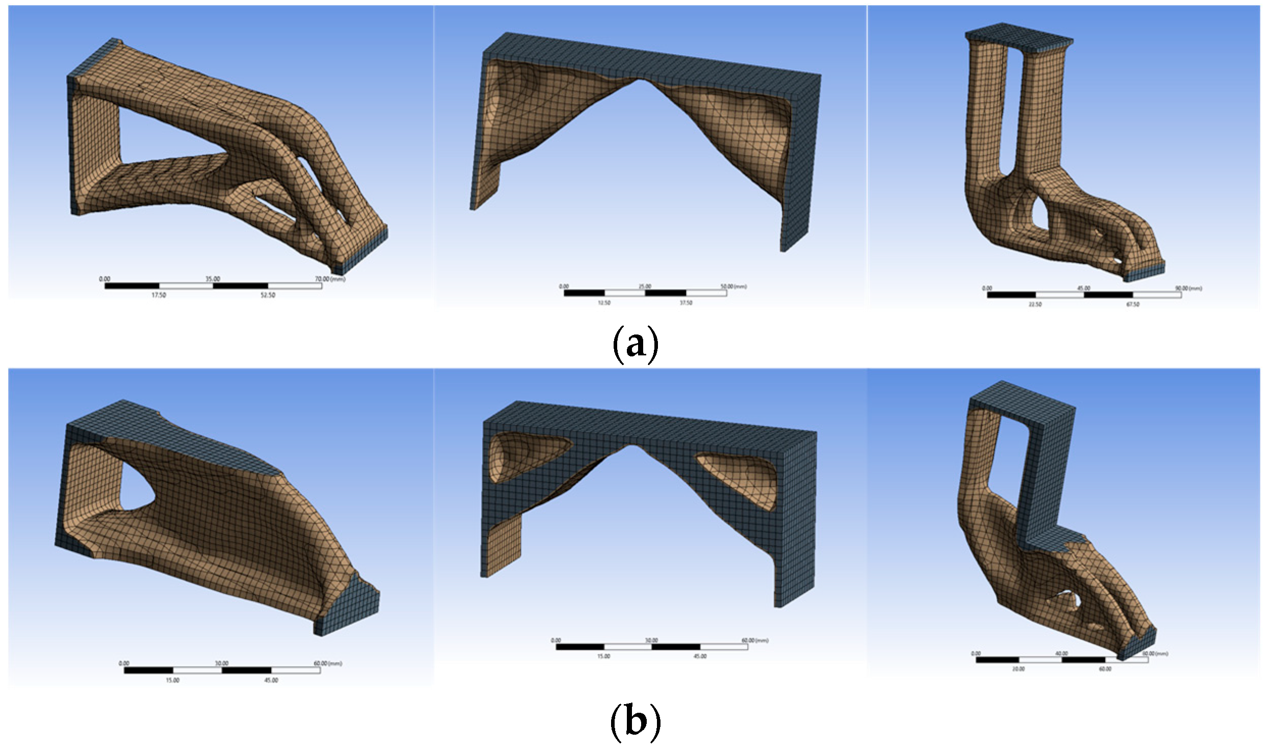
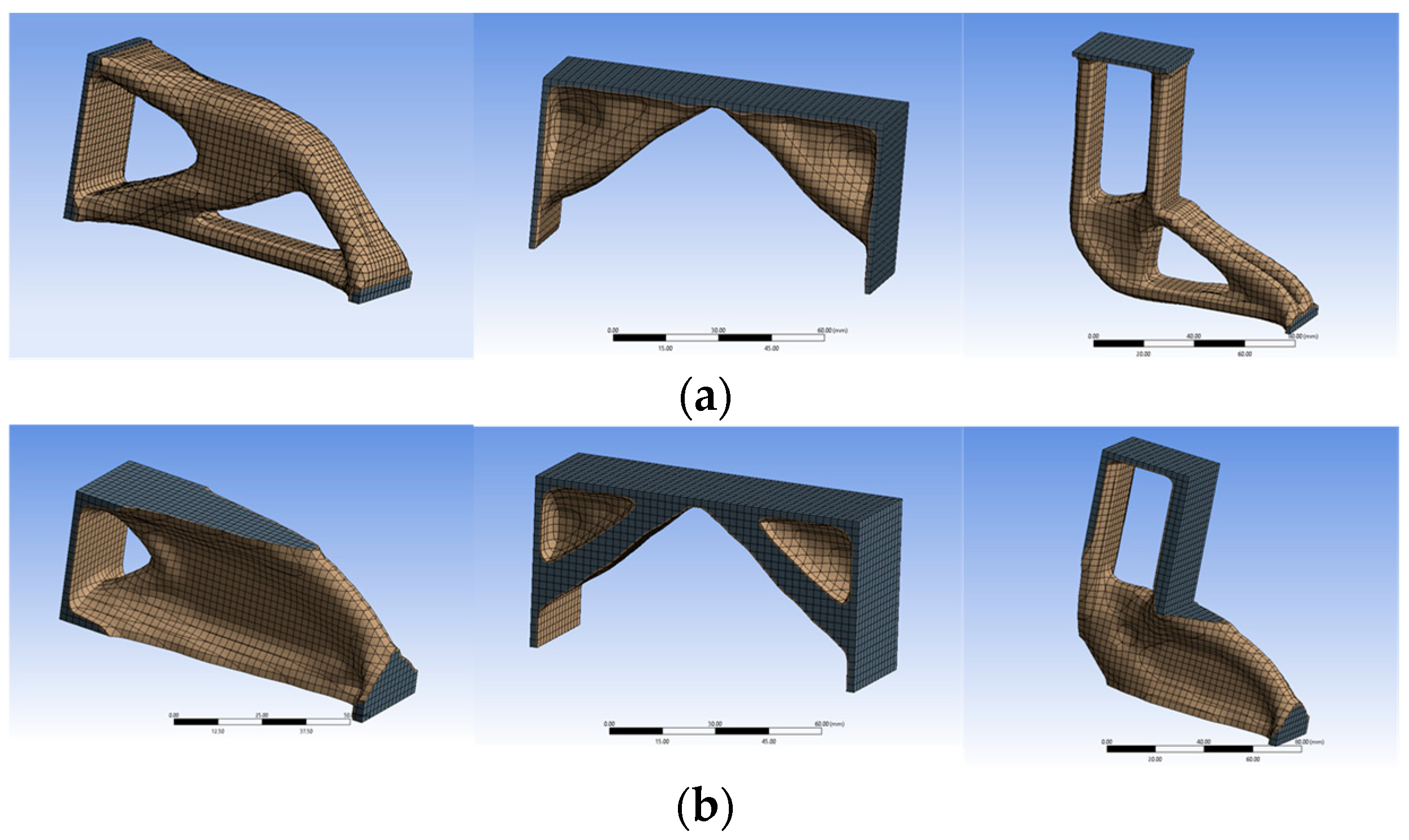
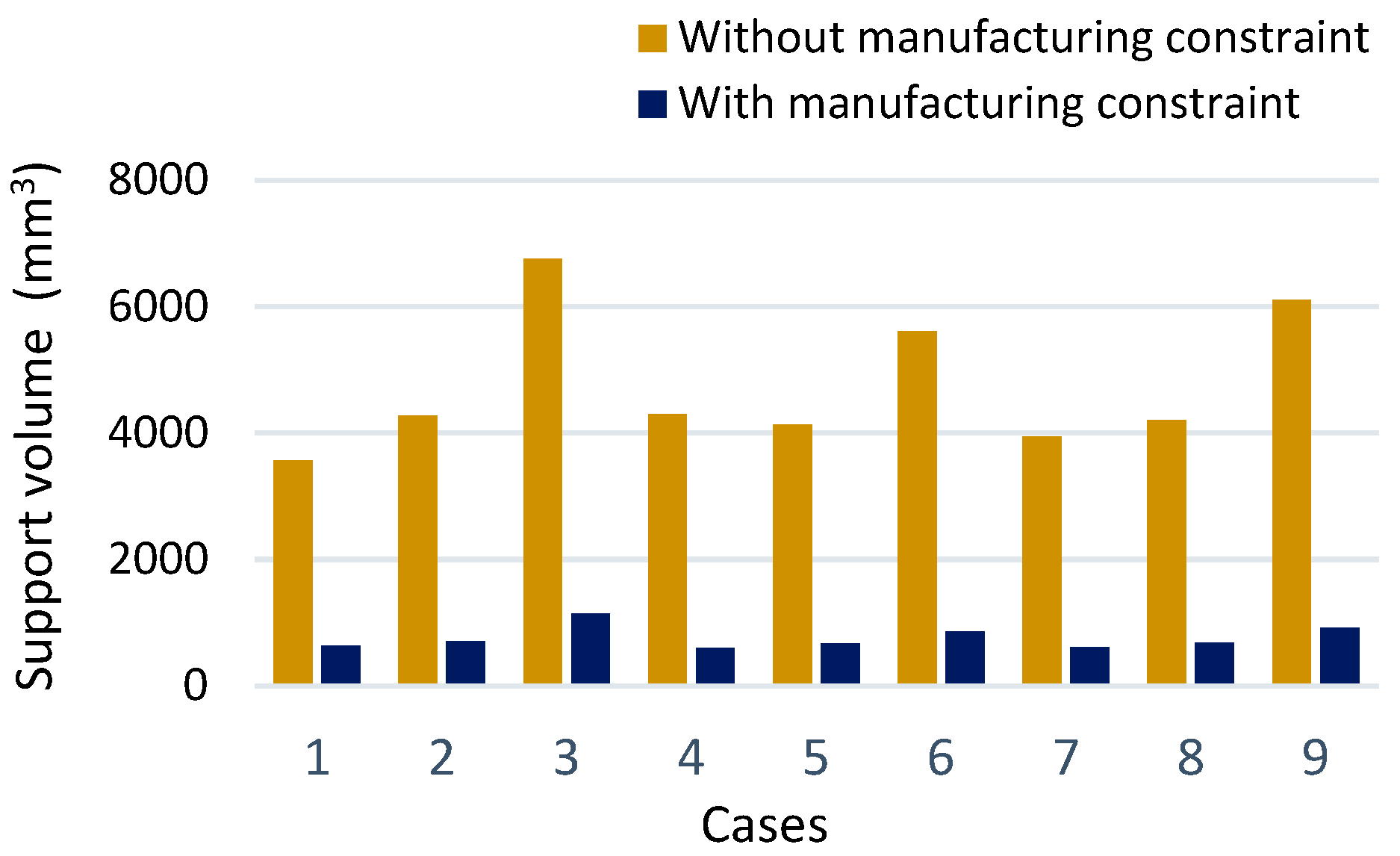
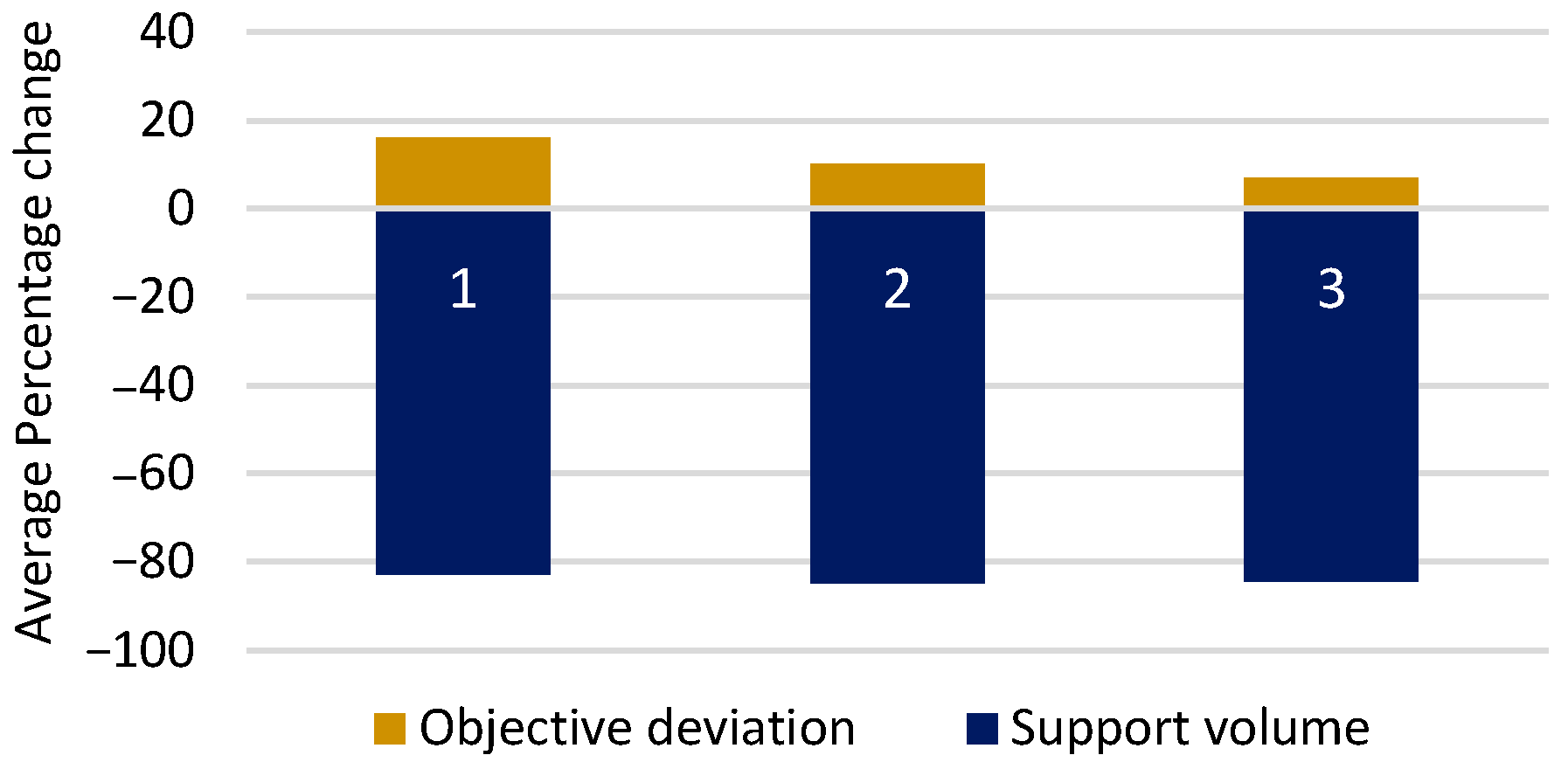
3.2. Effects of AM Constraints and Objective Functions

In this section, the impact of different objective functions on the structural topology optimization for AM is analyzed. To provide comprehensive insights, three different cases are considered: the cantilever beam, bridge shape, and L-shaped beam. For each case, the results are presented for topology optimization in different scenarios, with or without AM constraints. Based on the results shown in Table 2, −X is selected as the build orientation for the cantilever beam, and +Y is preferred for the bridge shape and the L-beam.

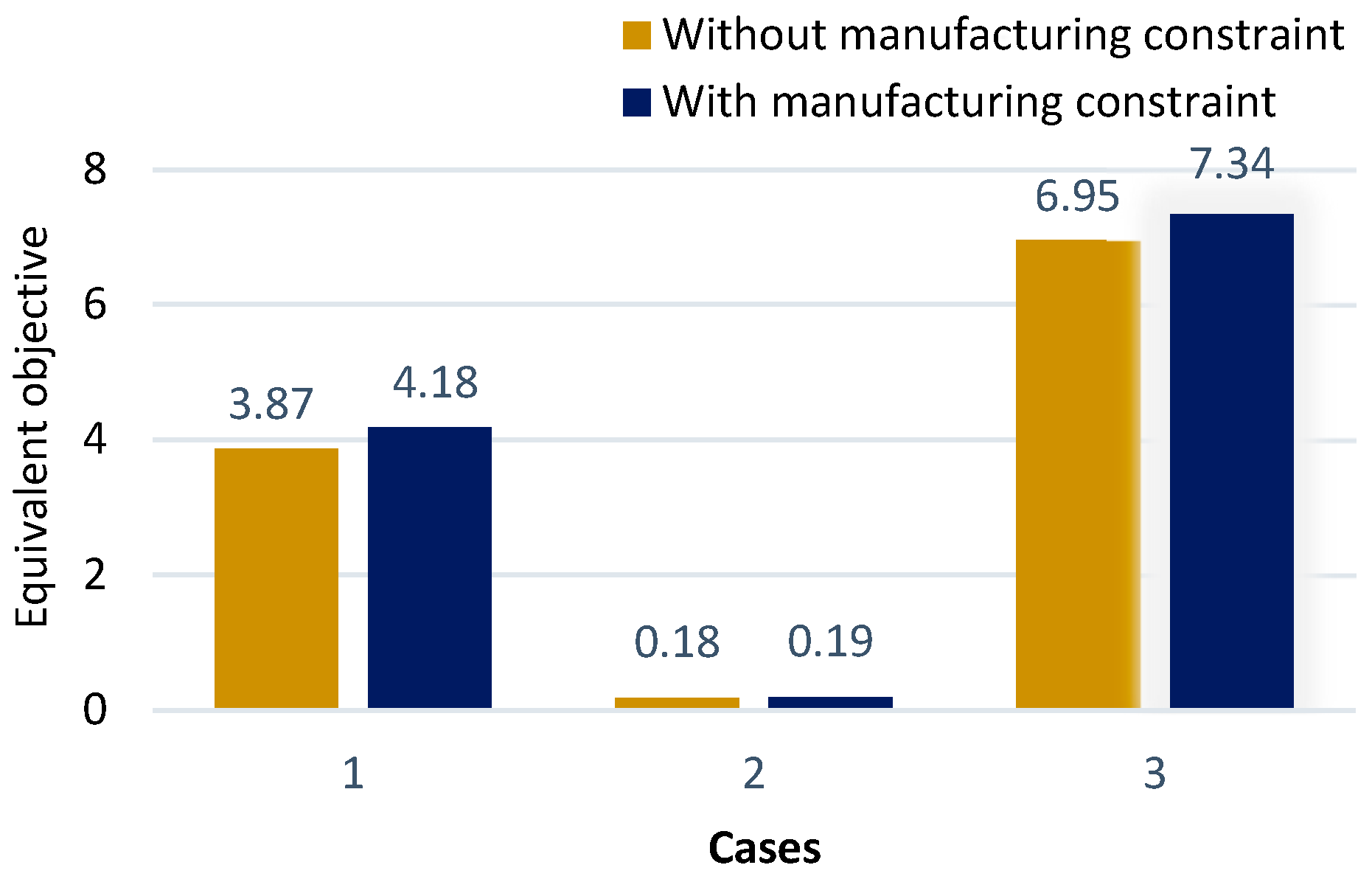
3.2.1. Compliance Minimization

Figure 10 shows a comparison plot of the compliance minimization results obtained from the topology optimization process, comparing the results with and without the inclusion of AM constraints. It is noteworthy that the introduction of AM constraints leads to an increase in compliance for all three designs analyzed. The increase in compliance when adding AM constraints is due to the increase in design change requirements to meet printing limitations. On average, compliance increases by 16.19% when AM constraints are considered, indicating the need to adapt the designs to meet the requirements of AM processes.

While under the influence of AM constraints, the average support structure volume decreases by 82.96%. This reduction in the support structure volume contributes to the overall decrease in the total volume. The reduction in the total volume achieved using the application of AM constraints demonstrates the potential for material efficiency and cost savings in AM.

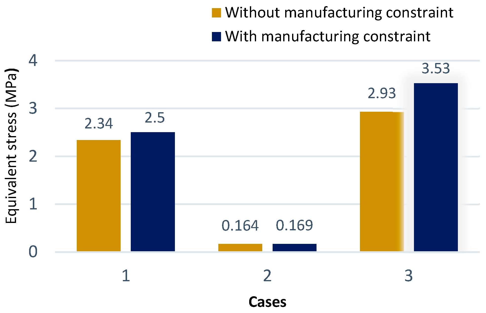
3.2.2. Stress Minimization

The stress minimization process was performed for all three designs in the presence and absence of AM constraints. Figure 11 shows that there is an increase in stress for all designs when AM constraints are included. On average, the stress increases by 10.16% due to the influence of AM constraints. The design validation result also shows that the equivalent stress slightly increases slightly when AM constraints are considered. However, it is important to note that despite this increase, the average support volume required under AM constraints decreased significantly by 84.81%.

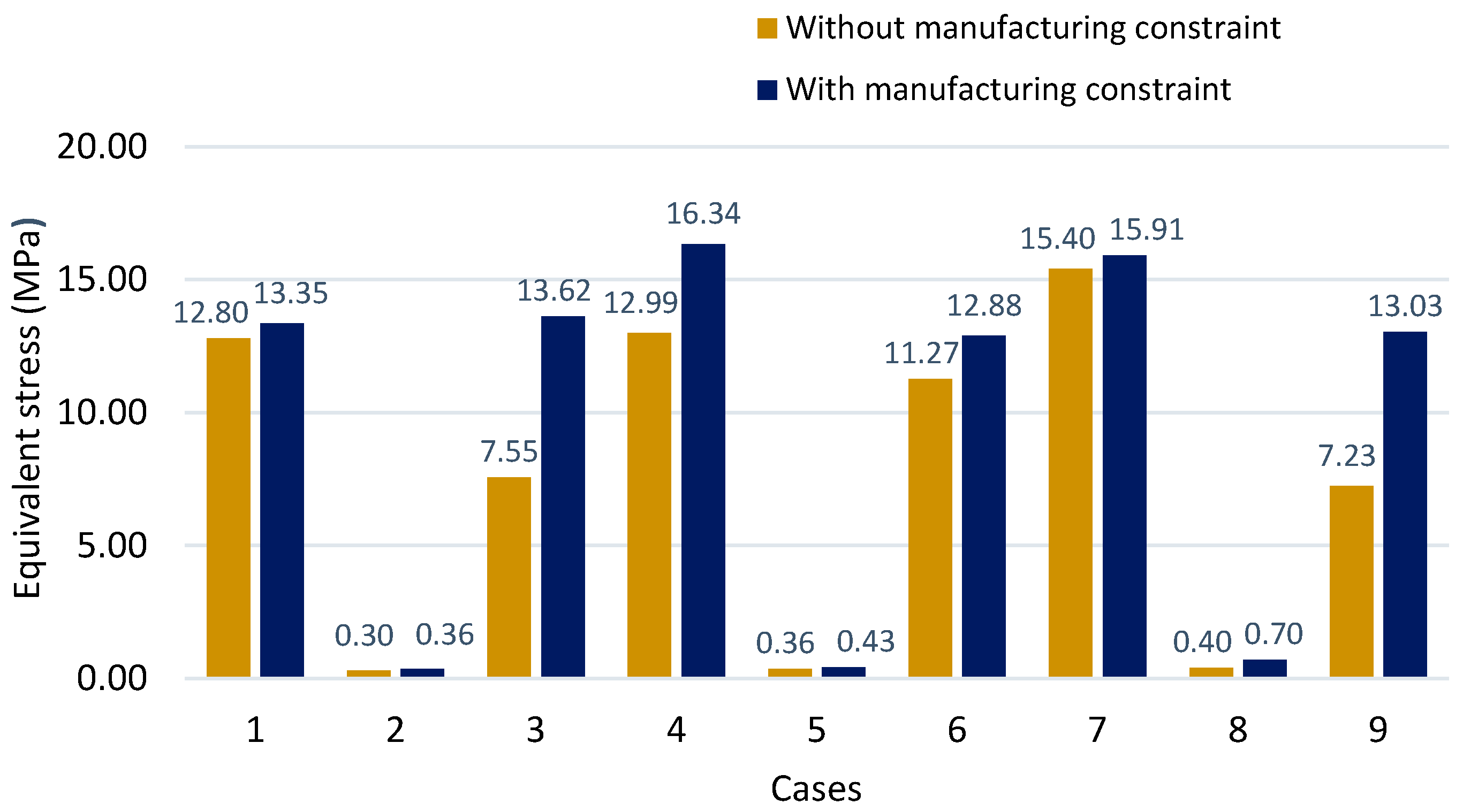
3.2.3. Compliance and Stress Minimization

The weighted sum method is utilized for topology optimization to minimize compliance and stress simultaneously, and the multi-objective function for stress and compliance is defined as:

$$f\left(x\right)=\frac{c\left(x\right)}{c_0}{w}_1+\frac{s\left(x\right)}{s_0}{w}_2$$

(18)

where f(x) is the objective function, and s(x) and c(x) are the stress and compliance functions for the physical density variable x. w₁ and w₂ are the weight combinations set to w₁ = 5 and w₂ = 1 for multi-objective optimization, and this weight combination was chosen based on the reference [28]. The relative importance of the two design objectives can be controlled in the overall objective function by multiplying each objective term by different weight factors, which would give designers more flexibility in terms of the area of application. As seen in Figure 12, it is observed that stress and compliance increase slightly when AM constraints are applied. The average increase in the multi-objective function value is 6.89%, while the average support volume required under this condition decreases by 84.36%.

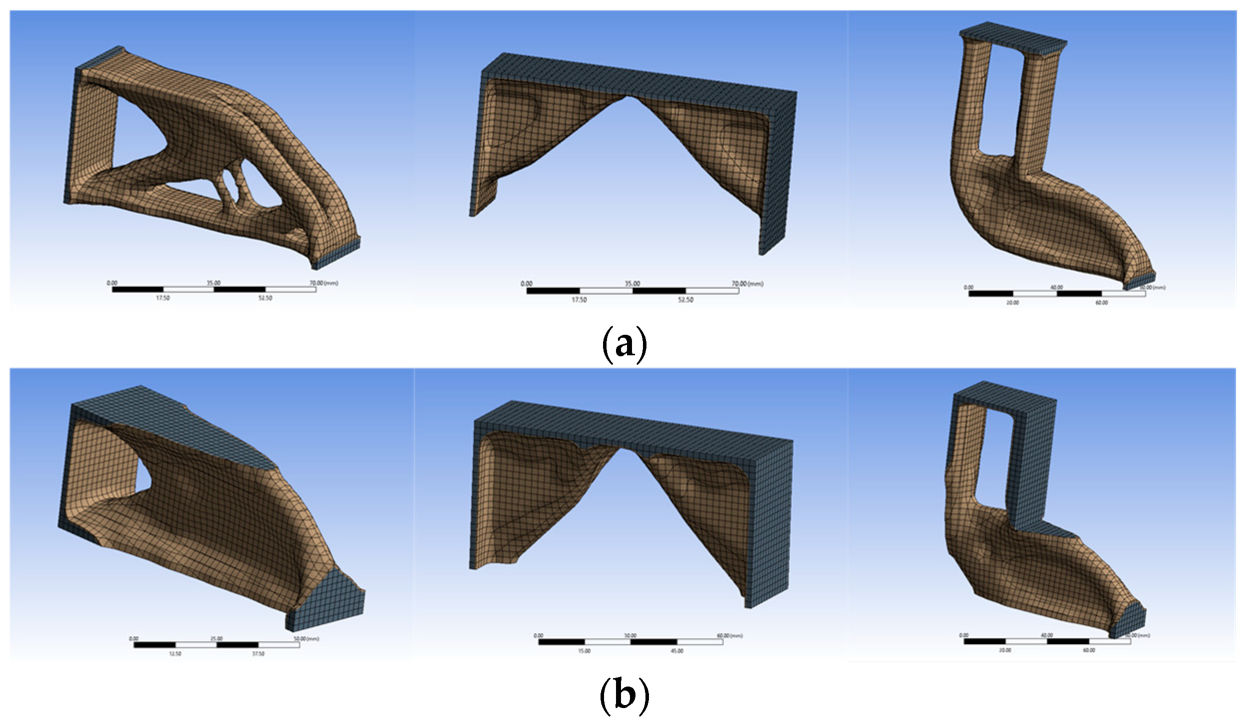
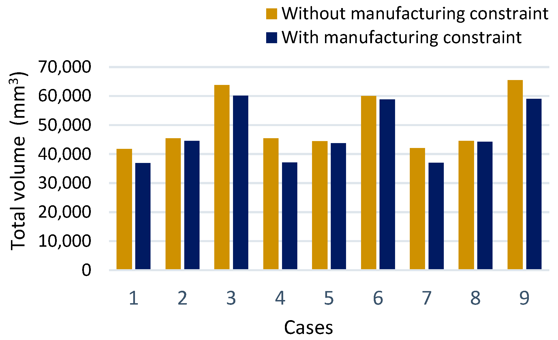
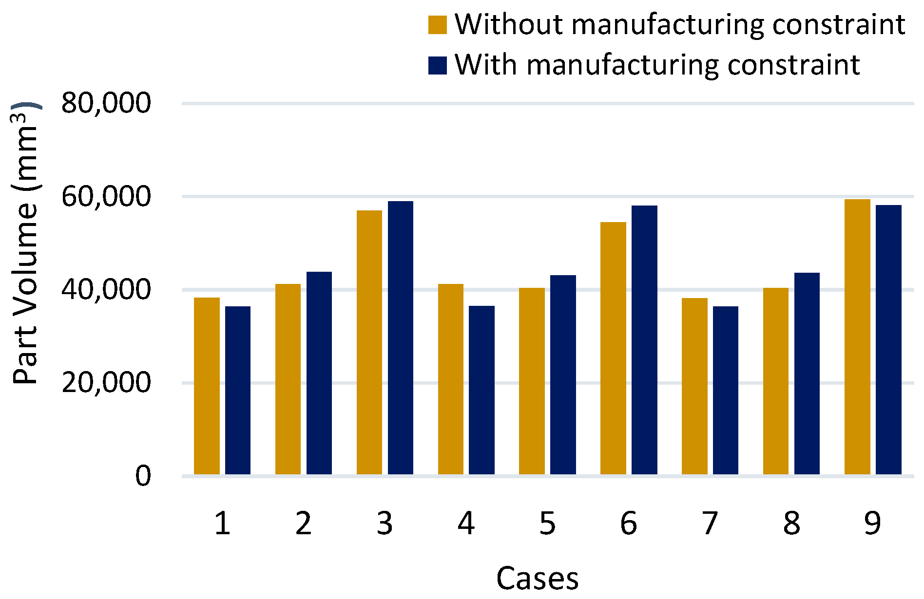
3.3. Comparative Study

When the AM constraints such as overhang and member size are used, the objective values for compliance, stress, and the multi-objective (stress and compliance minimization) formulations all increase compared to optimization without AM constraints. The design validation results for all three objectives show that the maximum equivalent stresses in each optimized case are similar and within the ultimate material limit, as seen in Figure 13. It is observed that the equivalent stress increases in all three cases when AM constraints are applied, as shown in Figure 14, Figure 15 and Figure 16. Among the three different objective formulations, the highest average objective increase is observed in compliance minimization, with an increase of 16.19%, while stress and compliance minimization have the lowest deviation increase of 6.89%. Overall, it is worth noting that adding AM constraints has the effect of increasing the value of the objective function, regardless of the type of design objectives.

The total volume after optimization without AM constraints is higher than that with AM constraints, as seen in Figure 17, while there are slight variations in the part volumes depending on the design configurations in Figure 18. This is because the required support structure was significantly reduced, as shown in Figure 19. The average reduction in support volume was similar for all three cases, with the compliance minimization having the lowest support volume reduction of 82.96% and the stress minimization having the highest reduction of 84.38%, as seen in Figure 20.

However, in certain cases, the optimizer may converge to a part geometry that has an increase in part volume in order to achieve a reduction in the volume of the support structure. This phenomenon can be observed in cases 2, 3, 5, 6, and 8 in Figure 18, where the optimizer converged to part geometries with increased volume to achieve a reduction in the support structure volume. Consequently, although the optimization process with AM constraints resulted in a significant reduction in support volume, the total volume of the design remained relatively unchanged. The optimizer tended to converge towards overly simplified shapes in order to minimize the support structures when AM constraints were added, as seen in Figure 14, Figure 15 and Figure 16. This is because the topology optimization with AM constraints prioritized minimizing support structures over exploring more intricate designs to reduce part volume. Thus, topology optimization was performed to increase additive manufacturability and reduce printing complexity. These results show that there is a trade-off relationship between part volume and support structure volume during the optimization process. While the reduction in support volume is desirable, the increase in part volume may limit the potential benefits of AM.

4. Closing Remarks

In this work, the effects of AM constraints and three different design objectives (i.e., compliance, stress, and multi-objective) on structural topology optimization were investigated. It was found that the build orientation plays a significant role when considering AM constraints in topology optimization, although its effectiveness varies depending on part geometries. The inclusion of AM constraints increased the optimal value of the objective function in the topology optimization but significantly reduced the required support structure volume. Comparing the results of the three different objective formulations, it was found that the average objective increase was the highest under compliance minimization (i.e., 16.19%), while the stress and compliance minimization had the lowest deviation increase (i.e., 6.89%). The average reduction in support volume was similar for all three cases. The reduction in the support volume demonstrates the potential for material efficiency and cost savings in AM. In the cantilever and L-shaped beam examples, the topology optimizer converged to more simplified shapes to reduce support structures when AM constraints were added. Depending on specific part geometries, it is likely that the part volume will increase to reduce the support structure volume, so the total volume, including part and support structure volumes, may remain relatively unchanged.

References

1. Rosen, D. Design for additive manufacturing: Past, present, and future directions. J. Mech. Des. 2014, 136, 090301. [Google Scholar] [CrossRef]
2. Zegard, T.; Paulino, G.H. Bridging topology optimization and additive manufacturing. Struct. Multidiscip. Optim. 2016, 53, 175–192. [Google Scholar] [CrossRef]
3. Mirzendehdel, A.M.; Suresh, K. Support structure constrained topology optimization for additive manufacturing. Comput.-Aided Des. 2016, 81, 1–13. [Google Scholar] [CrossRef]
4. Bruggi, M.; Duysinx, P. Topology optimization for minimum weight with compliance and stress constraints. Struct. Multidiscip. Optim. 2012, 46, 369–384. [Google Scholar] [CrossRef]
5. Liu, J.; Gaynor, A.T.; Chen, S.; Kang, Z.; Suresh, K.; Takezawa, A.; Li, L.; Kato, J.; Tang, J.; Wang, C.C.L.; et al. Current and future trends in topology optimization for additive manufacturing. Struct. Multidiscip. Optim. 2018, 57, 2457–2483. [Google Scholar] [CrossRef]
6. Meng, L.; Zhang, W.; Quan, D.; Shi, G.; Tang, L.; Hou, Y.; Breitkopf, P.; Zhu, J.; Gao, T. From topology optimization design to additive manufacturing: Today’s success and tomorrow’s roadmap. Arch. Comput. Methods Eng. 2020, 27, 805–830. [Google Scholar] [CrossRef]
7. Zhu, J.; Zhou, H.; Wang, C.; Zhou, L.; Yuan, S.; Zhang, W. A review of topology optimization for additive manufacturing: Status and challenges. Chin. J. Aeronaut. 2021, 34, 91–110. [Google Scholar] [CrossRef]
8. Ficzere, P. Effect of 3D printing direction on manufacturing costs of automotive parts. Int. J. Traffic Transp. Eng. 2021, 11, 94–101. [Google Scholar]
9. Langelaar, M. Topology optimization of 3D self-supporting structures for additive manufacturing. Addit. Manuf. 2016, 12, 60–70. [Google Scholar] [CrossRef]
10. Gaynor, A.T.; Guest, J.K. Topology optimization considering overhang constraints: Eliminating sacrificial support material in additive manufacturing through design. Struct. Multidiscip. Optim. 2016, 54, 1157–1172. [Google Scholar] [CrossRef]
11. Fritz, K.; Kim, I.Y. Simultaneous topology and build orientation optimization for minimization of additive manufacturing cost and time. Int. J. Numer. Methods Eng. 2020, 121, 3442–3481. [Google Scholar] [CrossRef]
12. Zhang, K.; Cheng, G.; Xu, L. Topology optimization considering overhang constraint in additive manufacturing. Comput. Struct. 2019, 212, 86–100. [Google Scholar] [CrossRef]
13. Brackett, D.; Ashcroft, I.; Hague, R. Topology Optimization for Additive Manufacturing. In Proceedings of the 2011 International Solid Freeform Fabrication Symposium, Austin, TX, USA, 8–10 August 2011. [Google Scholar]
14. Leary, M.; Merli, L.; Torti, F.; Mazur, M.; Brandt, M. Optimal topology for additive manufacture: A method for enabling additive manufacture of support-free optimal structures. Mater. Des. 2014, 63, 678–690. [Google Scholar] [CrossRef]
15. Bi, M.; Tran, P.; Xie, Y.M. Topology optimization of 3D continuum structures under geometric self-supporting constraint. Addit. Manuf. 2020, 36, 101422. [Google Scholar] [CrossRef]
16. Zhang, W.; Zhong, W.; Guo, X. An explicit length scale control approach in SIMP-based topology optimization. Comput. Methods Appl. Mech. Eng. 2014, 282, 71–86. [Google Scholar] [CrossRef]
17. Wang, X.; Zhang, C.; Liu, T. A topology optimization algorithm based on the overhang sensitivity analysis for additive manufacturing. IOP Conf. Ser. Mater. Sci. Eng. 2018, 382, 032036. [Google Scholar] [CrossRef]
18. Zhao, D.; Li, M.; Liu, Y. A novel application framework for self-supporting topology optimization. Vis. Comput. 2021, 37, 1169–1184. [Google Scholar] [CrossRef]
19. Jankovics, D.; Gohari, H.; Tayefeh, M.; Barari, A. Developing topology optimization with additive manufacturing constraints in ANSYS®. IFAC-PapersOnLine 2018, 51, 1359–1364. [Google Scholar] [CrossRef]
20. Gunwant, D.; Misra, A. Topology optimization of sheet metal brackets using ANSYS. MIT Int. J. Mech. Eng. Educ. 2012, 2, 120–126. [Google Scholar]
21. Bendsøe, M.P.; Kikuchi, N. Generating optimal topologies in structural design using a homogenization method. Comput. Methods Appl. Mech. Eng. 1988, 71, 197–224. [Google Scholar] [CrossRef]
22. Andreassen, E.; Clausen, A.; Schevenels, M.; Lazarov, B.S.; Sigmund, O. Efficient topology optimization in MATLAB using 88 lines of code. Struct. Multidiscip. Optim. 2011, 43, 1–16. [Google Scholar] [CrossRef]
23. Sigmund, O. Design of Material Structures Using Topology Optimization. Ph.D. Thesis, Technical University of Denmark, Lyngby, Denmark, 1994. [Google Scholar]
24. Neves, M.M.; Sigmund, O.; Bendsøe, M.P. Topology optimization of periodic microstructures with a penalization of highly localized buckling modes. Int. J. Numer. Methods Eng. 2002, 54, 809–834. [Google Scholar] [CrossRef]
25. Ansys. Ansys Blog—Simulation & Engineering Articles. Available online: https://www.ansys.com/blog (accessed on 10 March 2023).
26. Huei-Huang, L. Finite Element Simulations with Ansys Workbench 2021; SDC Publications: Misson, KS, USA, 2021. [Google Scholar]
27. Johnson, E. STL File Reader. Available online: https://www.mathworks.com/matlabcentral/fileexchange/22409-stl-file-reader (accessed on 25 February 2023).
28. Mhapsekar, K.; McConaha, M.; Anand, S. Additive manufacturing constraints in topology optimization for improved manufacturability. J. Manuf. Sci. Eng. 2018, 140, 051017. [Google Scholar] [CrossRef]
Figure 1. Neighborhood for the element and the filter size.
Applsci 13 10161 g001
Figure 2. Initial design domain for topology optimization: (a) Cantilever beam; (b) Bridge-shaped structure; and (c) L-shaped beam.
Applsci 13 10161 g002
Figure 3. Loading conditions: (a) Cantilever beam; (b) Bridge shape; and (c) L-beam.
Applsci 13 10161 g003
Figure 4. Setup for design validation.
Applsci 13 10161 g004
Figure 5. Optimized cantilever beams in six different build orientations.
Applsci 13 10161 g005
Figure 6. Optimized bridge-shape structures in six different build orientations.
Applsci 13 10161 g006
Figure 7. Optimized L-shaped beams in six different build orientations.
Applsci 13 10161 g007
Figure 8. L-shaped beam in the −Y build direction with (a) 50% and (b) 80% volume fraction.
Applsci 13 10161 g008
Figure 9. (a) New loading condition of the L-beam; (b) Optimal result along the −X build direction; (c) Optimal result along the −Y build direction.
Applsci 13 10161 g009
Figure 10. Compliance Minimization (1: cantilever, 2: bridge shape, 3: L-shaped beam).
Applsci 13 10161 g010
Figure 11. Stress Minimization (1: cantilever, 2: bridge shape, 3: L-shaped beam).
Applsci 13 10161 g011
Figure 12. Compliance and Stress Minimization (1: cantilever, 2: bridge shape, 3: L-shaped beam).
Applsci 13 10161 g012
Figure 13. Stress comparison (1, 4, 7: cantilever; 2, 5, 8: bridge shape; 3, 6, 9: L-shaped beam).
Applsci 13 10161 g013
Figure 14. Compliance minimization (a) without AM constraints and (b) with AM constraints.
Applsci 13 10161 g014
Figure 15. Stress minimization (a) without AM constraints and (b) with AM constraints.
Applsci 13 10161 g015
Figure 16. Compliance and stress minimization (a) without AM constraints and (b) with AM constraints.
Applsci 13 10161 g016
Figure 17. Comparison of the total volume after optimization (1, 4, 7: cantilever; 2, 5, 8: bridge shape; 3, 6, 9: L-shaped beam).
Applsci 13 10161 g017
Figure 18. Comparison of the part volume (1, 4, 7: cantilever; 2, 5, 8: bridge shape; 3, 6, 9: L-shaped beam).
Applsci 13 10161 g018
Figure 19. Comparison of the support structure volume (1, 4, 7: cantilever; 2, 5, 8: bridge shape; 3, 6, 9: L-shaped beam).
Applsci 13 10161 g019
Figure 20. Average change in design objectives and support structure volume between the optimization with and without AM constraints (1: compliance minimization, 2: stress minimization, 3: compliance and stress minimization).
Applsci 13 10161 g020