Abstract
In the Formula Student Racing Car, the frame is a fundamental component that supports the body. The frame’s anti-deformation ability will impact the four-wheel positioning parameters of the car, which subsequently affect the car’s stability. The quality of the frame directly determines the power and efficiency of the racing car, making the frame crucial to the overall race performance. Therefore, researching lightweight frame design is particularly important to enhance frame performance and reduce its total weight. In this paper, based on the variable density method, the global topology optimization of the frame is carried out to obtain the distribution of the frame material, realize the efficient utilization of the material, and improve the torsional stiffness of the frame. Compared with the previous local topology optimization, the global topology optimization involves a wider range, and the results are more accurate. Based on the adjoint variable method, the sensitivity analysis of the frame is carried out to obtain the influence level of each design variable. The size of the frame is optimized according to the variables with high influence levels. After optimization, the total mass of the frame is reduced by 12.8%; the performance in terms of maximum displacement and maximum stress is improved; and the lightweight design of the frame is realized as a whole.
1. Introduction
The Formula Society of Automotive Engineers (FSAE) is a prestigious university-level student design competition that focuses on the design and manufacturing of small, high-performance racing cars. It draws participation from countless college students worldwide every year. To date, hundreds of schools have enthusiastically taken part in this competition [1,2,3].
The participants focus on developing simple, lightweight, and easy-to-operate open-chassis vehicles while ensuring compliance with FSAE rules. To achieve this goal, various teams have conducted in-depth research on the design of racing frames to improve racing performance. Currently, research on racing frame design includes the following aspects: (1) reducing racing car resistance. Vaidya et al. conducted aerodynamic analysis and design on FSAE racing cars using fluid dynamics to reduce air resistance [4]. (2) Adopting new materials. Gui et al. studied the application of lightweight, high-stiffness, and high-strength materials such as carbon fiber and resin in racing, resulting in high power and safety performance during the race [5]. (3) Structural design of racing car frames. Yu Haiyan et al. designed a carbon fiber monocoque body with a total weight of 24.3 kg, which reduces the mass by 34% compared to the truss-type body. At the same time, by matching the laying direction, laying sequence, and laying quantity reasonably, the body achieves higher mechanical properties [6]. (4) The lightweight design of the frame. Hu Li et al. utilized the finite element method to design a truss frame for a college student racing car. Their approach successfully reduced the mass while maintaining the required strength and stiffness levels [7]. Similarly, Kong Deying et al. employed finite element analysis software to conduct topology design and size optimization on the frame. They effectively achieved significant weight reduction while ensuring compliance with constraints related to vehicle vibration frequency, strength, stiffness, and more [8].
The optimization of the racing frame involves two aspects: structural optimization and dimensional optimization. In terms of structural optimization, the commonly used approach is topology optimization. This method aims to identify the optimal material distribution within the given structural design domain, applied load, fixed boundary conditions, and constraints of the frame to enhance its performance indicators [9,10,11]. Topology optimization, as a highly effective conceptual design method, employs a model that maximizes stiffness [12]. This enables the frame to achieve the best load transmission path while maintaining high computational efficiency.
Among them, the homogenization design method is a multi-scale method that finds the best macroscopic structure by designing microstructure geometry with spatial variation. The principle is based on reducing the variation range of the material and adjusting the structure through a certain strategy to achieve homogenization. Specifically, the homogenization method in topology optimization is usually applied to the penalty term or objective function of the optimization process, which is achieved by introducing some items related to material homogenization [13].
There is another topological method for continuum structures: the variable density method. With the unit density in the design space as the design variable, the initial discrete value topology optimization problem is established as an optimization problem based on continuous design variables. It allows for the addition of effective materials to the structure while removing inefficient materials, resulting in an optimal structure [14]. By using the Solid Isotropic Material with Penalization (SIMP) method, the penalty factor p is introduced to increase the cost of intermediate-density elements and reduce the number of intermediate-density elements to make the density of elements as close as possible to 0 or 1 [15,16], which highlights the overall structure of the vehicle frame. In the design process, the initial density distribution is not necessarily uniform. Therefore, some methods need to be adopted in the design process to achieve a uniform distribution of density. Common homogenization methods include the volume fraction method, sensitivity analysis, and topological gradient method. These methods basically use some rules to balance the mass distribution of different units and achieve homogenization. Although density-based topology optimization has significant advantages in optimization time, material utilization, and reliability, its application still faces some challenges. For example, optimizing the nonlinear behavior of materials and special boundary conditions in complex regions can help solve these challenges. More importantly, in the solution module, the applicability of the variable density method is more extensive.
There are also some modern CAD-compatible topology optimization methods, such as the method based on non-uniform rational basis spline entities [17]. This can generate high-precision three-dimensional models with high efficiency and excellent computational performance. The geometric projection method realizes the distribution of materials and the filling of voids by dividing the optimization domain into grids and projecting them onto geometry [18]. The topology optimization method with a completely missing movable deformable gap and movable deformable component [19] is a new topology optimization algorithm that can be used to deal with holes and inherent scaling problems in topology optimization. It can effectively eliminate the empty area while maintaining the strength and stiffness of the structure. It will be a major challenge to apply these methods to formula racing in the future.
In terms of size optimization, the main issue is the large number of design variables. When optimizing dimensions, sensitivity analysis is added to select variables with larger influencing factors from numerous variables, and optimization design is carried out on these variables to improve the efficiency and effectiveness of size optimization.
Design sensitivity is the partial derivative of the design response to the optimization variable. From the perspective of calculation, the numerical methods of sensitivity analysis mainly include the following: the finite difference method, the direct differential method, and the adjoint variable method [20]. The finite difference method is a method based on numerical derivation that converts small changes in design variables into small changes in function values to calculate the sensitivity of design variables. In this method, numerical differentiation based on fractional differences is a common derivative technique. In addition, the finite difference method is not only suitable for calculating the sensitivity of one-dimensional and multi-dimensional functions but also for numerical models based on continuous and discrete variables. This method is simple, intuitive, and easy to implement, but in most cases, it needs to deal with very complex gradient calculations. The direct differential method is a method based on differential calculation. It calculates the differential between the design parameters and the system response by directly solving the analytical expression of the problem. The direct differential method can calculate the derivatives of multivariate functions more accurately, which makes it more widely used in nonlinear and dynamic systems. However, this method is computationally expensive, especially when the number of variables increases [21]. Due to the large number of frame fittings, there are many variables, so this method is not applicable. The adjoint variable method is a popular numerical method that is often used in sensitivity analysis and optimization problems. In this method, the objective function and constraint conditions of the optimization problem are represented as operators and vectors, which are used to calculate the partial derivatives of the design parameters. The main advantage of the adjoint variable method is that its computational complexity is much lower than that of the direct differential method, and it is widely used in engineering optimization and design because of its rapidity in calculation. However, for the nonlinear prediction model, its application range may be limited.
The optimization of the racing car frame plays an important role in improving the performance of the car. At present, more research has focused on the optimization of the frame. In recent years, many scholars have conducted some research on frame optimization. Wang et al. [22] considered the strength and mode of the frame under complex road conditions and improved the relevant parameters through optimization, but only the topology optimization was performed for the cockpit, and the mass became heavier. Lyduch et al. [23] used the optimization method SIMP to optimize the topology of some frame structures, which improved the modal performance. The frame mass was reduced by size optimization, but the design parameters were not determined by sensitivity analysis, so the size optimization was blind. Fu et al. [24] made the mechanical properties of the frame superior through optimization analysis and realized the lightweight of the frame. However, only the topology optimization of the front cabin was performed, and the sensitivity analysis was not used. David et al. [25] mainly improved the torsional stiffness through sensitivity analysis, but this method had not been applied in the field of lightweight design. To sum up, in the field of the formula racing car frame, most of the literature only does topology optimization on the local part, and the size optimization does not set the appropriate design variables, which is blindness. In addition, in international journals, many studies have applied sensitivity analysis to other parts of the car, such as [26,27,28]. In recent years, it has been difficult to find the application of sensitivity analysis in the field of lightweight frame design in the literature, so this research is essential for frame design.
The above papers are compared with the research in this paper, as shown in Table 1. The main contributions of this paper are as follows: (1) Global topology optimization of the frame based on the variable density method. Compared with the local topology optimization, the global topology optimization optimizes the frame of the cockpit and the rear cabin at the same time. The optimization results will retain the material in the area with higher unit density to obtain the trend of the whole vehicle pipe fittings, so that the designed frame structure is more accurate and the anti-deformation performance will be better. (2) The sensitivity analysis is introduced into the field of racing frames. The adjoint variable method is used to analyze the sensitivity of the frame, and the influence factors of each variable are obtained according to the results. The size of the frame is optimized based on the variables with greater influence. Compared with other sensitivity analysis methods, this method provides an effective way to calculate the gradient of design parameters and has a faster calculation speed. It can determine the best design parameters in a shorter time, explore a wider design space, and more effectively optimize the quality and performance of the frame. More importantly, it provides appropriate design parameters for size optimization and improves accuracy, so that the effect of lightweight design will be better. In the second section of this paper, the model establishment of the frame is introduced. The frame structure is simulated and analyzed by Hyper Works software under various working conditions. In Section 3, the topology optimization, sensitivity analysis, and size optimization of the frame are carried out, and the performance of the frame before and after optimization is compared to highlight the effect of optimization. Finally, the research is summarized in Section 4.

Table 1.
Literature research.
2. Frame Model Design and Structural Analysis
The frame is the “keel” of a racing car, providing positioning points for the transmission, steering, and suspension systems. Frame design is a key technology that plays an important role in automotive design. The high-performance frame of a racing car requires high torsional stiffness, as it directly affects the car’s turning performance [29]. Therefore, the frame design must fully consider the assembly of each component and the lightweight nature of the frame itself, ensuring that the frame can withstand various working conditions and enable the racing car to successfully complete its tasks. Taking into account factors such as design difficulty, repair difficulty, and manufacturing cost, this article selects a spatial truss structure for the frame and utilizes 4130 steel as the material choice.
2.1. Determine Geometric Modeling of Frame
- (1)
- Input the coordinates of suspension hard points in the CATIA V5 part design to create a suspension line diagram;
- (2)
- Determine the specific parameters of the main ring, front ring, and front partition;
- (3)
- Connect the bottom of the front partition, the bottom of the front ring, and the bottom of the main ring with lines in sequence;
- (4)
- Determine the slanted support structure for the main ring and its upper and lower slanted support structures;
- (5)
- Utilize the cockpit opening detection board and the cockpit internal cross-sectional detection board to verify whether the front cabin and cockpit of the frame meet the requirements of the competition rules.
2.2. Establishing Finite Element Model
2.2.1. Finite Element Theory
- (1)
- The structure is discretized, transforming the ductile continuous medium into a relatively limited number of simple basic elements. These elements are generated based on node connections, and the load is also transmitted through these nodes. Different types and numbers of elements can be selected during the entire process of discretization, which directly affects the accuracy and stability of the numerical values in the finite element analysis of the solid model;
- (2)
- After the discretization is constructed, to better represent the displacement, stress, and strain of the element with the nodal displacement, the displacement function formula can be used for description:
In the equation:
refers to the displacement column vector of a point in the element.
refers to the shape function matrix of the element.
refers to the node displacement column vector of an element.
According to the geometric equation in elasticity, the element strain correlation indicated by the element node displacement column vector is deduced:
In the equation:
refers to the strain column vector at any point in the element.
refers to the strain matrix of the element.
Based on the principle of virtual work, the relationship between node load and node displacement of the function on the element was created, and the bending stiffness equation of the element was derived:
where K refers to the stiffness matrix of the element, δ refers to all constructed node displacement space column vectors, and refers to the load column vector of the overall structure.
- (3)
- Solve, synthesize all bending stiffness equations, and obtain the equilibrium equations for all constructions, namely:
The bending stiffness equation is expressed as:
where is the Young’s modulus matrix, v is Poisson’s ratio, and C is the linear elastic stiffness matrix of the element.
In order to introduce the penalty parameter, E can be modified to obtain Young’s modulus matrix after penalty:
among them, is Young’s modulus matrix after penalty, is the design variable in topology optimization, and is the penalty parameter. By adjusting the penalty parameter, the continuity and optimization degree of the material can be controlled. When the penalty parameter approaches infinity, some parts of the material are disabled to optimize the structure. When is equal to 1, the continuity of the material is completely maintained.
2.2.2. Establishment Process
This article conducts simulation analysis and optimization design in the Hypermesh environment. The geometric model is imported into CATIA V5 to create the finite element analysis model. The steps are as follows:
- (1)
- Establishing materials: The frame is made of 4130 steel, also known as 30CrMo, with an elastic modulus of 2.0510 MPa, a Poisson’s ratio of 0.33, a density of 7.8510 g/cm3, and an allowable stress of approximately 390 MPa;
- (2)
- Unit selection: Using Hyperbeam, create a beam unit with a uniform outer diameter of 25.4 mm for pipes and individual pipes with an outer diameter of 20 mm. Following the rules of the competition frame design section, establish four different wall thicknesses for the steel pipes: 20 mm (outer diameter) × 2.2 mm (wall thickness), 25.4 mm × 2.4 mm, 25.4 mm × 1.65 mm, and 25.4 mm × 1.25 mm;
- (3)
- Establish attributes: Create four attributes with the same names as the previously established four beam elements (for easy matching). Ensure that they correspond one by one with the beam section;
- (4)
- Grid divisions: Divide the pipe fittings into grids and set the grid size to 10 mm for efficient calculation.
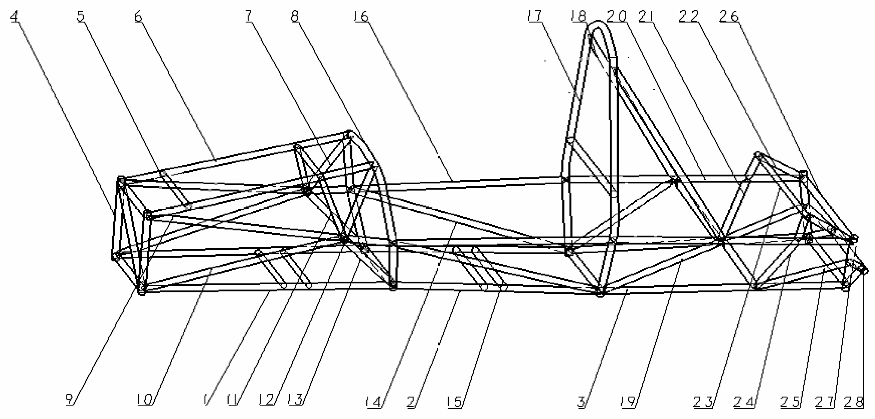
The established finite element model of the vehicle frame is shown in Figure 1.
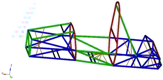
Figure 1.
Finite element model of the vehicle frame.
2.3. Working Condition Analysis
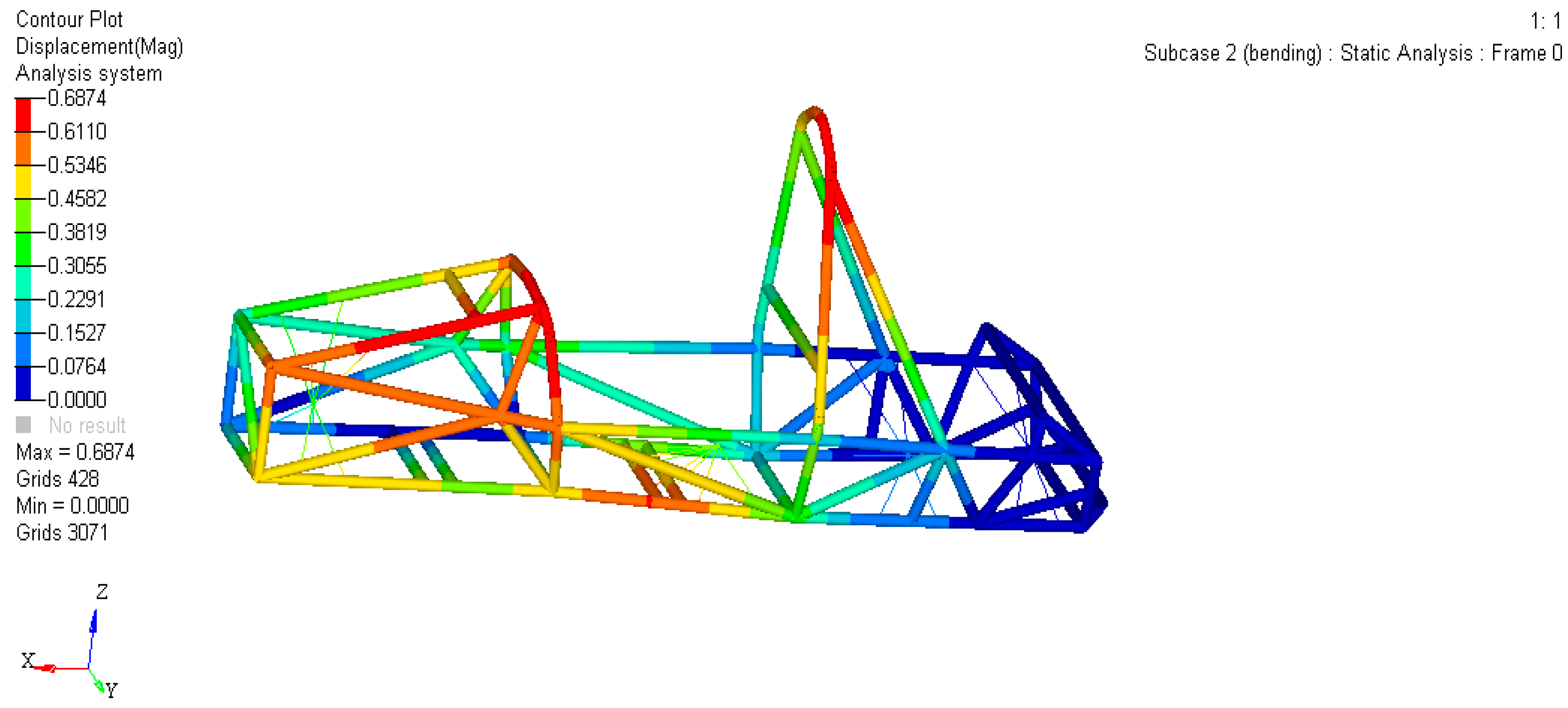
2.3.1. Bending Conditions
The bending condition is used to analyze the strength and stiffness of a racing car when all four wheels land simultaneously under full load, mainly simulating the stress distribution and deformation of a racing car driving at a uniform speed on a good road surface. Establish constraint conditions with a frame weight of approximately 45 kg and represent the vehicle weight by applying a gravity field. Set the gravity acceleration to 9.8 N/kg and input N3 to −1, indicating that the gravity field is loaded in the negative direction of the z-axis. Due to the relatively high speed under bending conditions, the dynamic load coefficient is taken as 2.0. Constrain the left and right front suspensions dof3, and constrain the left and right rear suspensions dof1, dof2, and dof3. Among them, dof1, dof2, and dof3 represent linear degrees of freedom along the x, y, and z axes, while dof4, dof5, and dof6 represent angular degrees of freedom around the x, y, and z axes. In the process of analyzing the working condition of the racing frame, the constraint condition is indispensable, mainly to constrain the force and various loads of the frame in the actual driving so that it will not be excessively bent or deformed and to ensure its stability and safety.
As shown in Figure 2 and Figure 3, dark blue to red represents the minimum to maximum stress or strain value. Among them, red is the area where stress or strain is mainly concentrated, and it is also the focus of attention. The maximum strain of the frame is 0.6874 mm, and the maximum pressure is 62.44 MPa.
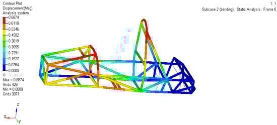
Figure 2.
Displacement cloud diagram of the frame under bending conditions.
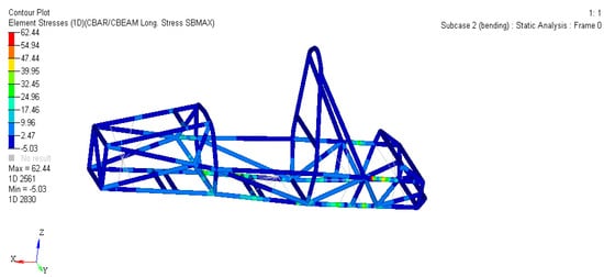
Figure 3.
Stress cloud diagram of the frame under bending conditions.
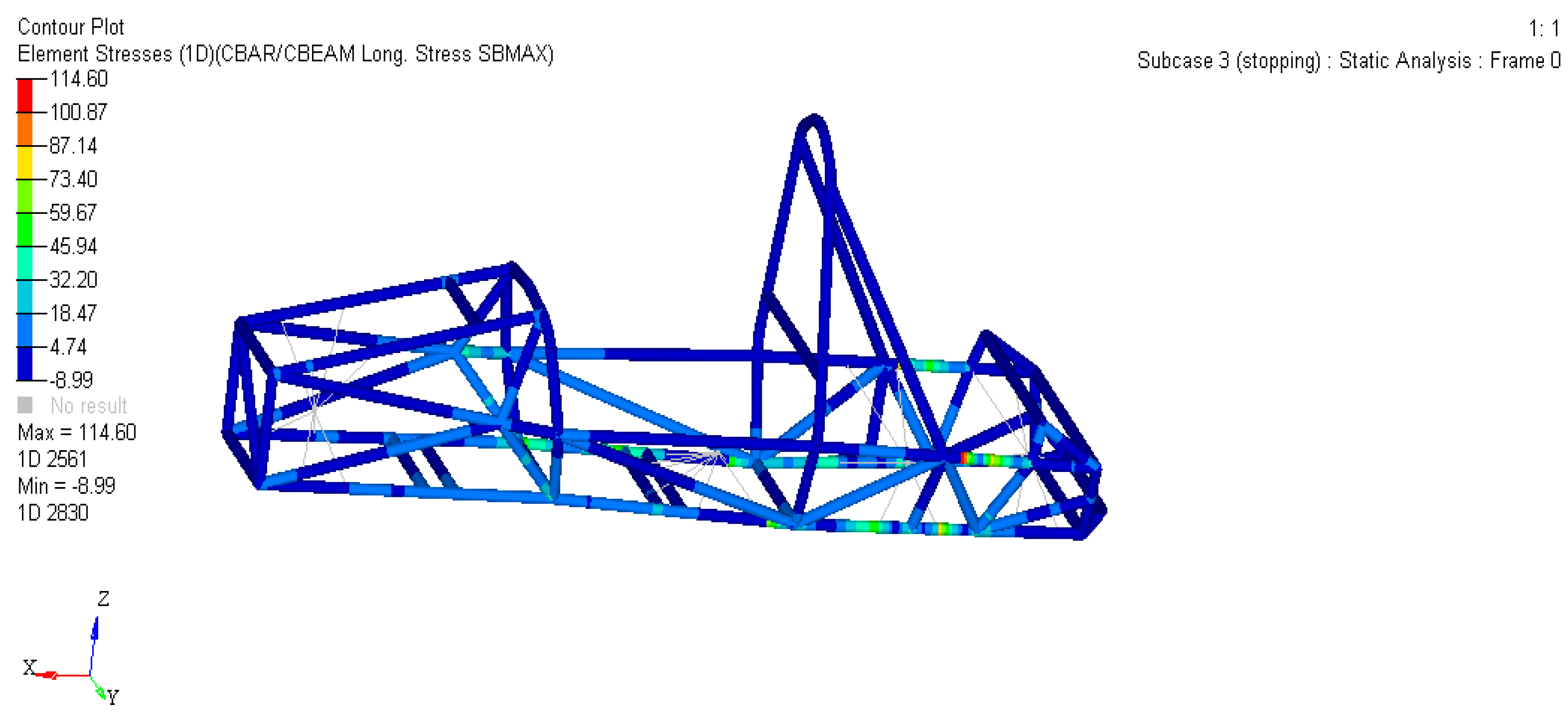
2.3.2. Emergency Braking Conditions
When a racing car brakes, the frame not only bears the same static load as the bending condition but also receives the longitudinal inertia force generated by the braking force at the contact point between the tire and the ground. Here, the dynamic load coefficient is taken as 2.0, and the braking deceleration is 1.4 g. The constraint conditions are the same as those of the full load bending condition.
As shown in Figure 4 and Figure 5, the maximum strain of the frame is 1.125 mm, and the maximum pressure is 114.6 MPa.
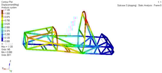
Figure 4.
Displacement cloud map of the frame under braking conditions.

Figure 5.
Stress cloud diagram of the frame under braking conditions.
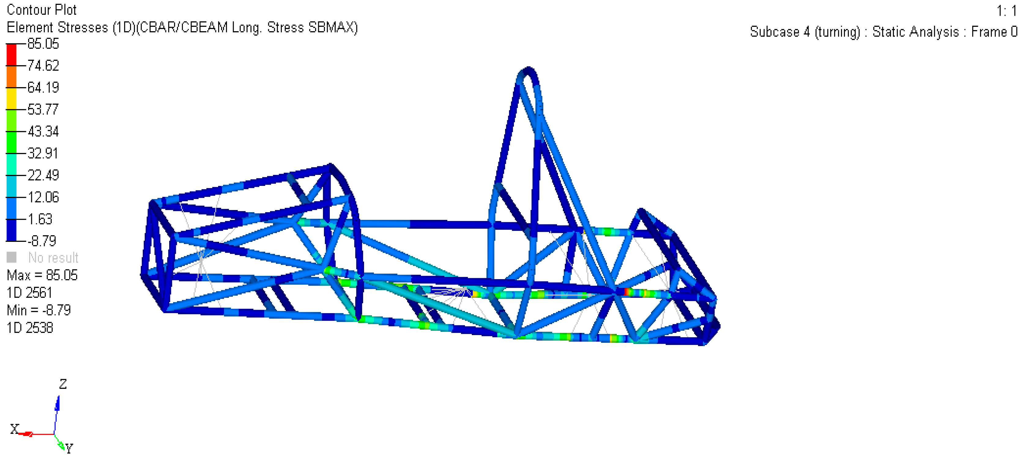
2.3.3. High-Speed Turning Conditions
When a racing car enters a corner, the frame not only bears the same static load as the bending condition but also undergoes lateral inertia under the action of centrifugal force. The magnitude of this inertia force depends on the vehicle speed, turning radius, road angle, etc. This condition corresponds to an eight-figure surround test. Taking a left turn as an example, the dynamic load coefficient is 1.5 and the centripetal acceleration is about 1 g. Constrain the left front suspension equivalent points dof1 and dof3, constrain the right front suspension equivalent points dof2 and dof3, and constrain the left and right rear suspension equivalent points dof3.
As shown in Figure 6 and Figure 7, the maximum strain of the frame is 0.8838 mm and the maximum pressure is 85.05 MPa.
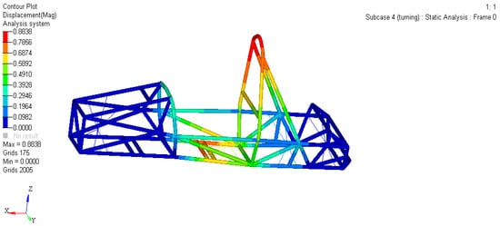
Figure 6.
Displacement cloud map of the frame under turning conditions.
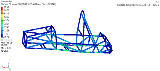
Figure 7.
Stress cloud diagram of the frame under turning conditions.
2.4. Analysis of Frame Structure Stiffness
The static stiffness of the frame mainly includes bending stiffness and torsional stiffness, which have a significant impact on the strength, vibration, noise, and fatigue characteristics of the frame. Generally speaking, the greater the stiffness of the frame, the greater its strength. For FSC racing frames, their strength is usually guaranteed by the rules, but their stiffness varies greatly. Therefore, it is necessary to analyze the stiffness of the frame, especially the torsional stiffness.
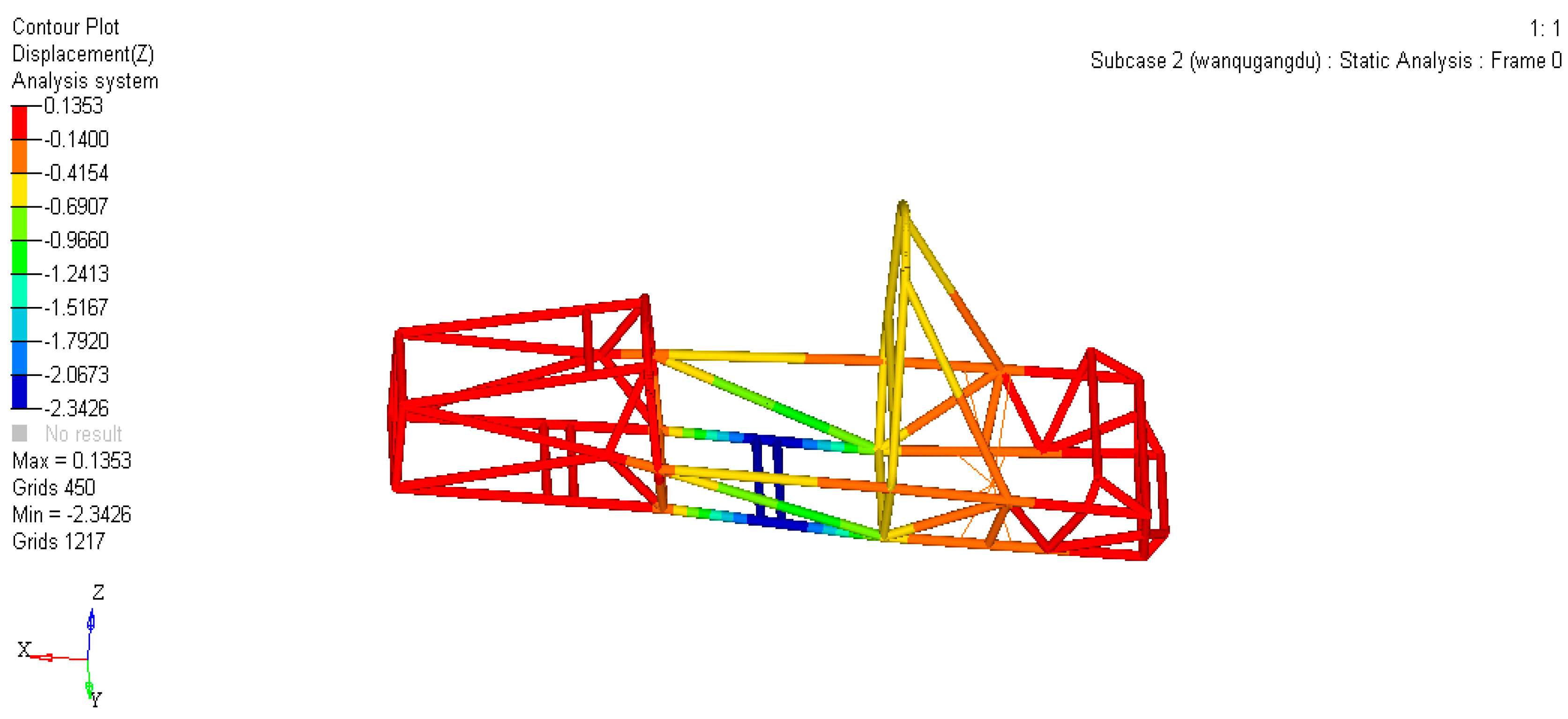
2.4.1. Bending Stiffness Analysis
On the basis of the finite element model of the frame bending condition, remove the driver’s mass and retain the motor’s mass. At the middle of the longitudinal beams on both sides of the cockpit bottom, a concentrated force F = 1000 N of equal magnitude and in the same direction (the negative direction of the Z-axis) is applied, and the constraint conditions and other settings are the same as the bending condition.
The solution result is shown in Figure 8, with a deflection value of 0.1353 mm in the vertical direction. Calculate the bending stiffness EI = F/Z = 7390 N/mm according to the formula (where F represents the bending load, Z represents the larger deflection value of the frame in the vertical direction, and EI represents the bending stiffness).

Figure 8.
Displacement variables of the frame in the z-axis direction.
2.4.2. Torsional Stiffness Analysis
Constrain the left rear suspension dof1 and dof3, constrain the right rear suspension dof1, dof2, and dof3, and release all dofs from the left and right front suspensions [30]. Apply a pair of equal and opposite concentrated forces F (left Z, right Z) to the equivalent points of the left and right front suspensions, where F = 1000 N.
The solution results in a significant deviation of 3.502 mm. Subsequently, the torsion angle between the two equivalent points of the front suspension was measured, and the result was 0.333° with a spacing of 490.008 mm. According to the formula K = T/θ, calculate the torsional stiffness of the frame with a value of 1471.5 Nm/°, where K denotes torsional stiffness and T and θ denote torque and torsional angle of view, respectively. After reviewing foreign design materials, it was found that the torsional stiffness range of the racing car is basically within the range of 1000–4000 Nm/° [31], indicating that the torsional stiffness design of the frame is reasonable.
2.5. Modal Analysis
2.5.1. Modal Analysis Theory
Modal analysis is the process of obtaining the modal vibration characteristics of a modal construction system. Each mode includes its inherent damping coefficient, modal frequency, modal shape, and other key parameters. The process of obtaining these basic parameters is called modal analysis. Based on modal analysis, on the one hand, the degree of influence between the supported component and the supporting component can be evaluated. On the other hand, as an evaluation indicator of dynamic characteristics, its modal frequency and mode shape can serve as a reference for dynamic changes. Therefore, conducting modal analysis on the frame is particularly important [32].
2.5.2. Calculation Process of Frame Mode
- (1)
- Establish a finite element model of the structure;
- (2)
- Set solution methods and control parameters;
- (3)
- Extracting modal results;
- (4)
- As shown in Table 2, the low-order modal frequency and modal shape of the frame are obtained through calculation. Among them, the frequencies before the first-order mode are all lower than 1 Hz, which corresponds to the six-degree-of-freedom rigid mode in free modal analysis. Therefore, considering the extraction from modes greater than 1 Hz as the first order, the result is that the lowest first-order frequency is approximately 36 Hz. The frame possesses a natural frequency, which refers to the frame’s elastic vibration frequency within a small range around its equilibrium state. When the frame experiences external excitation close to its natural frequency, resonance occurs, increasing the frame’s amplitude and consequently affecting the handling stability and driving safety of the vehicle. Generally, the frequency of road excitation is around 20 Hz, while the lowest first-order frequency of the frame is about 36 Hz. Thus, if the vehicle operates on a road with a frequency of around 20 Hz, it can avoid the frame’s natural frequency to a certain extent and prevent the occurrence of resonance effects.
Table 2. Frame-free modal analysis results.
3. Frame Optimization Design
3.1. Introduction to Topology Optimization Method
Topology is a way to improve the spread of materials in the design space under the constraints of the initial conditions and internal structural performance parameters. Among them, the variable density method is widely used in topology. It takes the unit density of each module in the design space as the design variable. In density-based topology optimization, the continuous density field ρ:Ω → [0, 1] is replaced by the constant density distribution of the element caused by the finite element discretization. Topological design is within the design domain ρ = 1. Void material ρ = 0 is described by the continuous variation of fictional unit density [33], but in reality, intermediate-density units cannot exist and cannot be manufactured. Therefore, it is necessary to avoid the generation of intermediate-density units as much as possible and reduce the number of intermediate-density units. In this case, it is necessary to penalize the intermediate density values that appear in the design variables. The most popular material interpolation model method currently is the SIMP method, which is represented by the formula:
In the equation:
—Elastic modulus after interpolation.
—Elastic modulus of material in the solid part.
—Elastic modulus of material in the porous part.
—Unit relative density, with a value of 1 indicating the presence of material and 0 indicating the absence of material or holes.
p—Penalty factor.
The higher the unit density, the more critical it is that the material at this location be retained, as it is responsible for bearing the load. Reduce the use of materials with low unit density, achieving lightweight design and rational utilization of materials.
The mathematical model of topology optimization can be expressed as [32]:
Minimize:
Constraints:
In the function, X represents the design variable, f (X) represents the objective function, represents inequality constraint functions, represents the equality constraint function, L represents the upper limit of the constraint, and U represents the lower limit of the constraint.
3.2. Topology Optimization of Frame
3.2.1. Topology Optimization Settings
- (1)
- Design variable: Unit density of the frame space;
- (2)
- Establish responses: Create responses such as weighted comp and mass, respectively;
- (3)
- Constraint condition: The mass of the frame design space is limited to 0.3–0.5, which means that the solved material mass accounts for 30–50% of the original mass (placement penalty factor);
- (4)
- Establish objective function: The optimization objective is flexibility, which is equivalent to the displacement formed by a unit force at that point in data, while stiffness is equivalent to the force required to cause a unit displacement at that point in data. Therefore, the objective function sets the minimum flexibility as the maximum stiffness;
- (5)
- Minimum and maximum member sizes: The minimum size needs to be greater than three times the size of the grid unit, and the maximum member size needs to be greater than two times the minimum member size. The measured unit distance is 13.15 mm, so the minimum size min-dim is set to 50 mm and the maximum size max-dim is set to 100 mm;
- (6)
- Symmetric constraint: The frame structure is symmetrical about the longitudinal plane. Since only the degrees of freedom of the left front suspension are fixed in the load step, a symmetric constraint about the xoz plane is applied in the design variables in order to simultaneously consider the right front suspension.
Based on the above settings, establish a topology model, as shown in Figure 9.
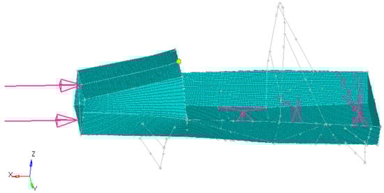
Figure 9.
Topological model of the frame.
3.2.2. Topology Optimization Results
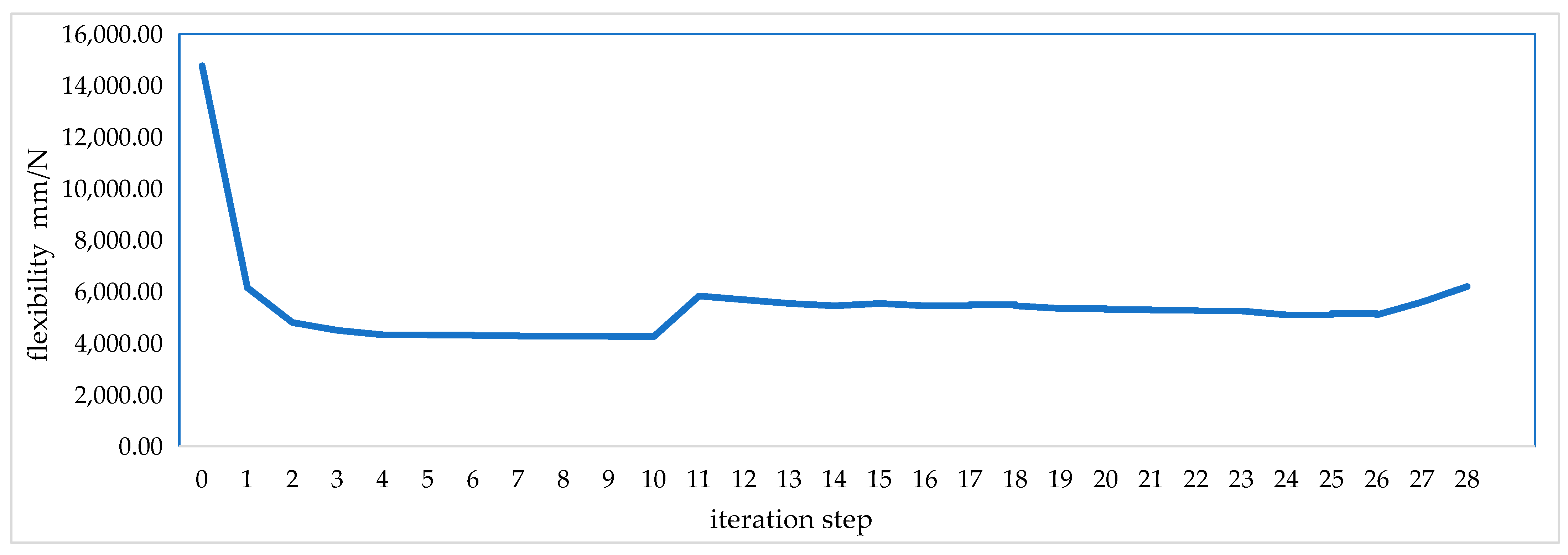
After 33 iterations, the calculation was completed, and the iteration frequency curve is shown in Figure 10. With the increase in iteration frequency, the flexibility maintained a decreasing trend, with the lowest points of flexibility being 4760 and 5100 in the 10th and 26th iterations, respectively.
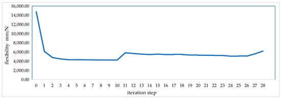
Figure 10.
Function image of flexibility change.
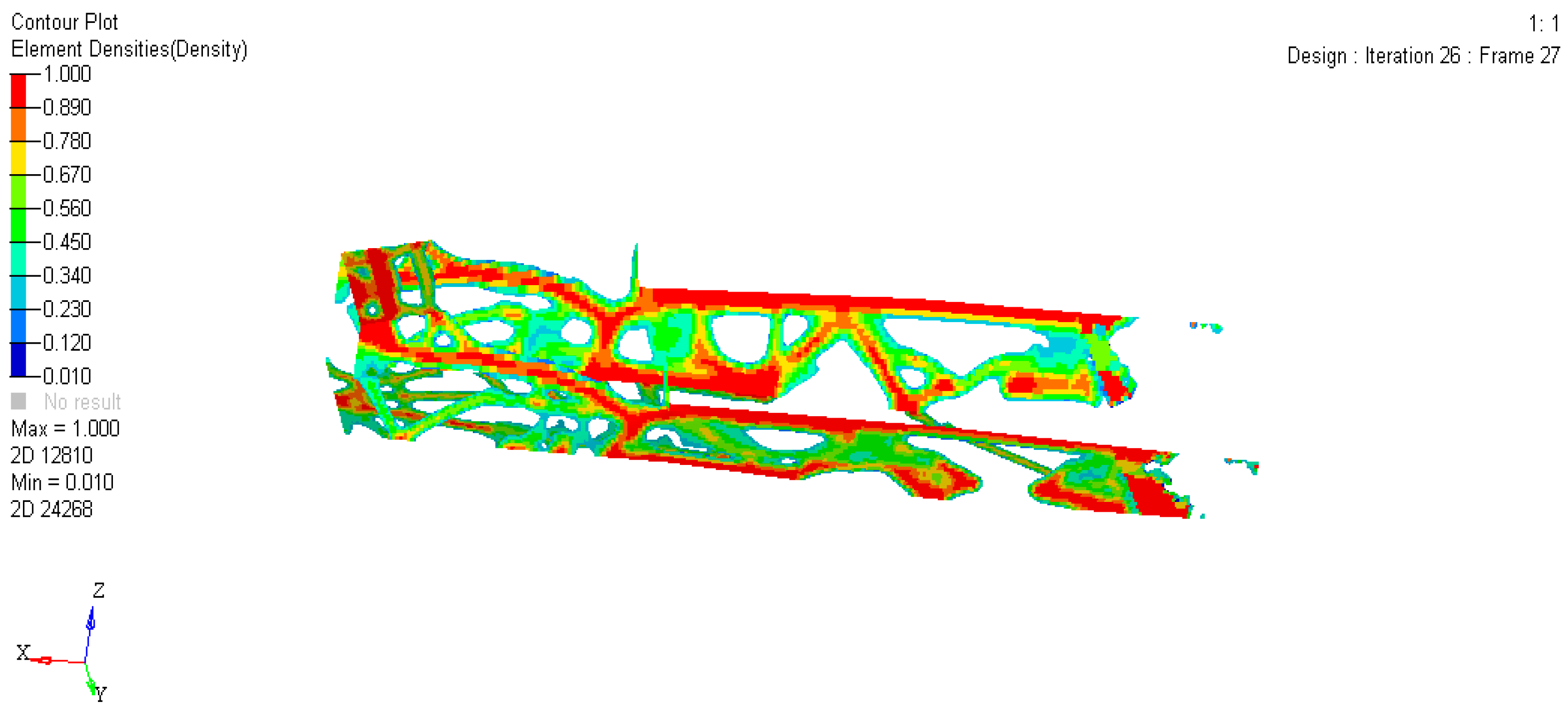
Pay attention to the iterative results of these two steps and obtain the material interpolation model based on the SIMP method, as depicted in Figure 11 and Figure 12. This is achieved by assigning intermediate densities to represent the obtained topological result while penalizing them. In the model, the bright red area corresponds to a unit density of 1, the dark blue area represents a unit density of 0, and the other shades represent intermediate densities.
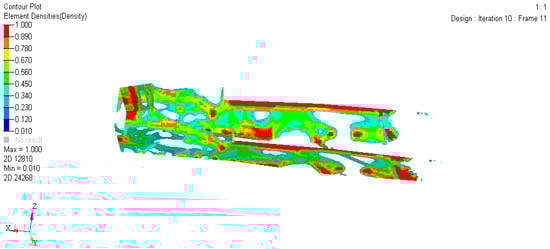
Figure 11.
The pattern after the iterative optimization solution is in step 10.
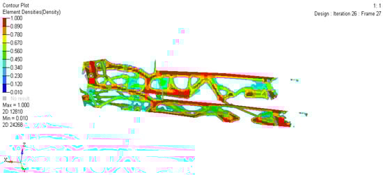
Figure 12.
The pattern after the iterative optimization solution is in step 26.
These two resolved patterns represent the material distribution of the frame. The area with a unit density of 1 serves as the main component of the frame, responsible for load transmission, while the areas with intermediate densities represent other components of the frame.
Through comprehensive analysis of Figure 10, Figure 11 and Figure 12, it is observed that although the flexibility in the iterative operation of Step 10 is slightly smaller than that in Step 26, the difference is not significant. Considering the material distribution effect, Step 26 yields the best result with a more pronounced material distribution. Therefore, the difference in flexibility is disregarded, and the iterative result obtained in Step 26 is selected as the final result of topology optimization.
Finally, some adjustments are made to the pipe fittings based on the results of the topology optimization. As shown in Figure 13, a solid line indicates the addition of a pipe fitting in the front compartment. In the frame structure considered in this paper, the main body comprises thin-walled circular steel tubes. Designing solely based on the results of topology optimization would lead to practical manufacturing issues and non-compliance with competition rules. Thus, it becomes necessary to incorporate manufacturability treatment, which involves combining the optimization result with actual processing technology and modifying it based on engineering experience. This ensures that the optimized frame can be manufactured smoothly and meets the requirements set by the competition rules. Figure 14 illustrates the addition of a pipe fitting to the front partition support structure, while Figure 15 depicts the removal of a pipe fitting from the rear compartment (represented by a dashed line).
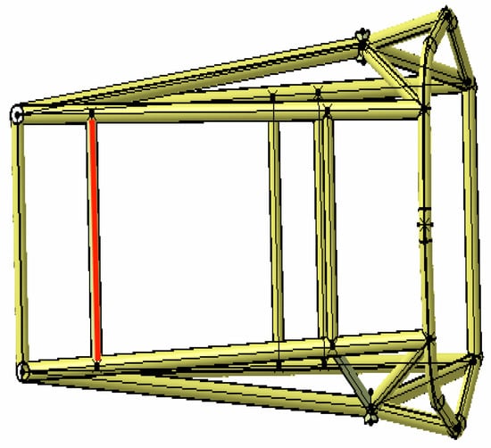
Figure 13.
Front compartment model after topology optimization.
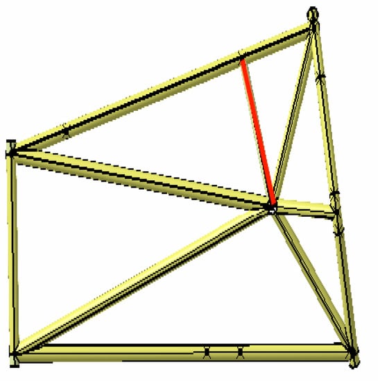
Figure 14.
Front diaphragm support structure after topology optimization.
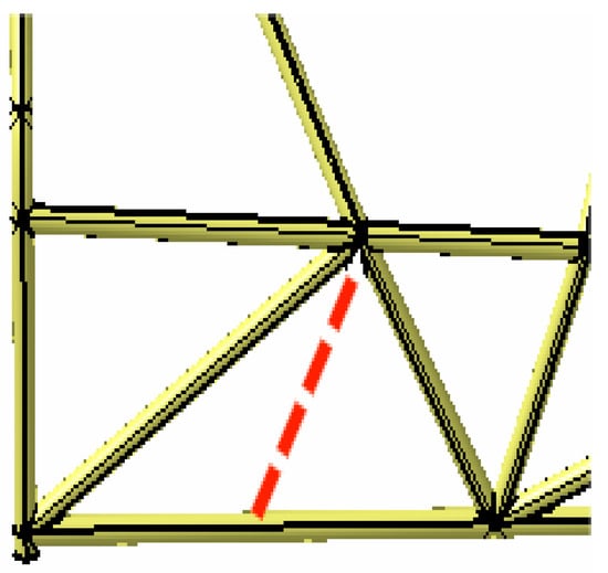
Figure 15.
Rear compartment model of the frame after topology optimization.
3.3. Size Optimization
3.3.1. Sensitivity Analysis
The sensitivity analysis of the frame involves examining the impact of changes in technical parameters on design variables. It is performed based on the optimization design approach. By conducting sensitivity analysis, we can determine the level of influence that design variables have on the design response, which helps in clarifying improvement plans. Sensitivity refers to the partial derivative of the design response with respect to a particular design variable. It represents the extent of change in the objective function when the design variable is altered, and the weight of the variable is obtained through this sensitivity. Design sensitivity, on the other hand, refers to the partial derivative of the design response with respect to optimization variables. For optimization problems with a large number of design variables and fewer constraints, such as topology optimization and topography optimization, the adjoint variable method can be used to calculate sensitivity. The adjoint variable method enables the simultaneous processing of multiple variables. When there are more design variables than responses, the adjoint variable method proves to be more efficient compared to other methods. This feature makes it particularly suitable for analyzing sensitivity issues in large structures [34]. In the following sections, the method will be described in detail.
- (1)
- Solving the original finite element model: According to the geometric parameters and material parameters of the original finite element model, the numerical solution of the target physical quantity represented by the displacement field is obtained by solving the static, dynamic, or steady-state analysis problems. This numerical solution is used to solve the following adjoint problem;
- (2)
- Establish the motion balance equation: There is a relationship between the structural performance parameter g and displacement as follows:where K represents the stiffness matrix and represents the load space vector of a unit node.
- (3)
- Lagrange equation: According to the Lagrange equation, the kinematic equation of the system is expressed as a differential equation of generalized coordinates and generalized velocities. The following formula is as follows:where is the Lagrange multiplier, the structural design variable , is the constraint function, and is the Lagrange function.
- (4)
- Solving the adjoint problem: Suppose there is the following relationship between the structural performance parameter g and the displacement:where represents the adjoint displacement vector and represents the vector of the element displacement node.
The sensitivity of the structural response to the structural design variable X is expressed as [35]:
- (5)
- Calculation of generalized displacement gradient: For the optimization problem with many design variables and few design tube bundles, the adjoint variable a is introduced to make
From Equations (12) to (16), it can be concluded that:
3.3.2. Optimization of Frame Size
The purpose of size optimization is to reduce the wall thickness of less stressed pipe fittings, thereby achieving a lightweight design (some pipe fittings are determined according to rules) and improving the power performance of racing cars.
- (1)
- Design variables: Use the inner and outer diameters of each pipe fitting on the frame as design variables. Because the frame is a symmetrical structure about the longitudinal plane, setting two symmetrical pipe fittings as a variable effectively improves computational efficiency. According to specific needs, the range of values for each variable should be clarified. The initial value of the inner circle radius for this racing frame is 10.3 mm, with a variation range of 1–14 mm. The initial value of the outer circle radius is 12.7 mm, with a variation range of 1–3 mm (as shown in Figure 16);
 Figure 16. Definition of design variables for size optimization.
 - (2)
- Establish responses: In the responses panel, establish three responses: mass, stress, and displacement;
- (3)
- Constraints: ① Because the maximum stress of the frame under three typical working conditions is 114.6 MPa, which is lower than the allowable stress and has a large optimization space, the maximum stress is set to not exceed 200 MPa. ② Respectively constrain the displacement to not exceed the original value under various working conditions; for example, the displacement does not exceed 0.3792 mm under bending conditions;
- (4)
- Set objective function: With the overall goal of minimizing the net weight of the vehicle frame, use the accuracy and output card provided in Hypermesh to define the accompanying variables and output sensitivity analysis results.
3.3.3. Analysis of Optimization Results
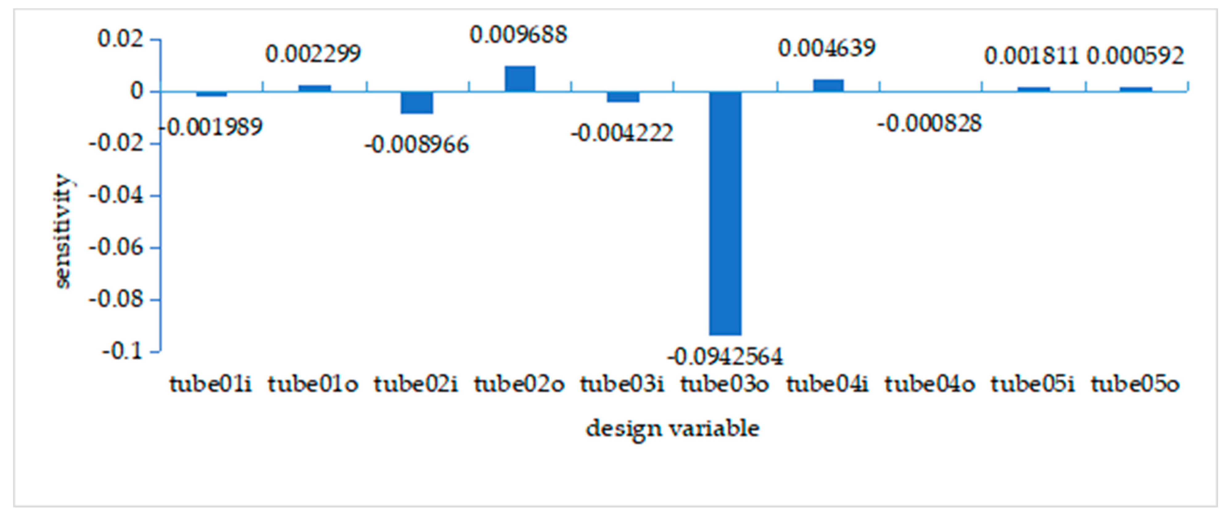
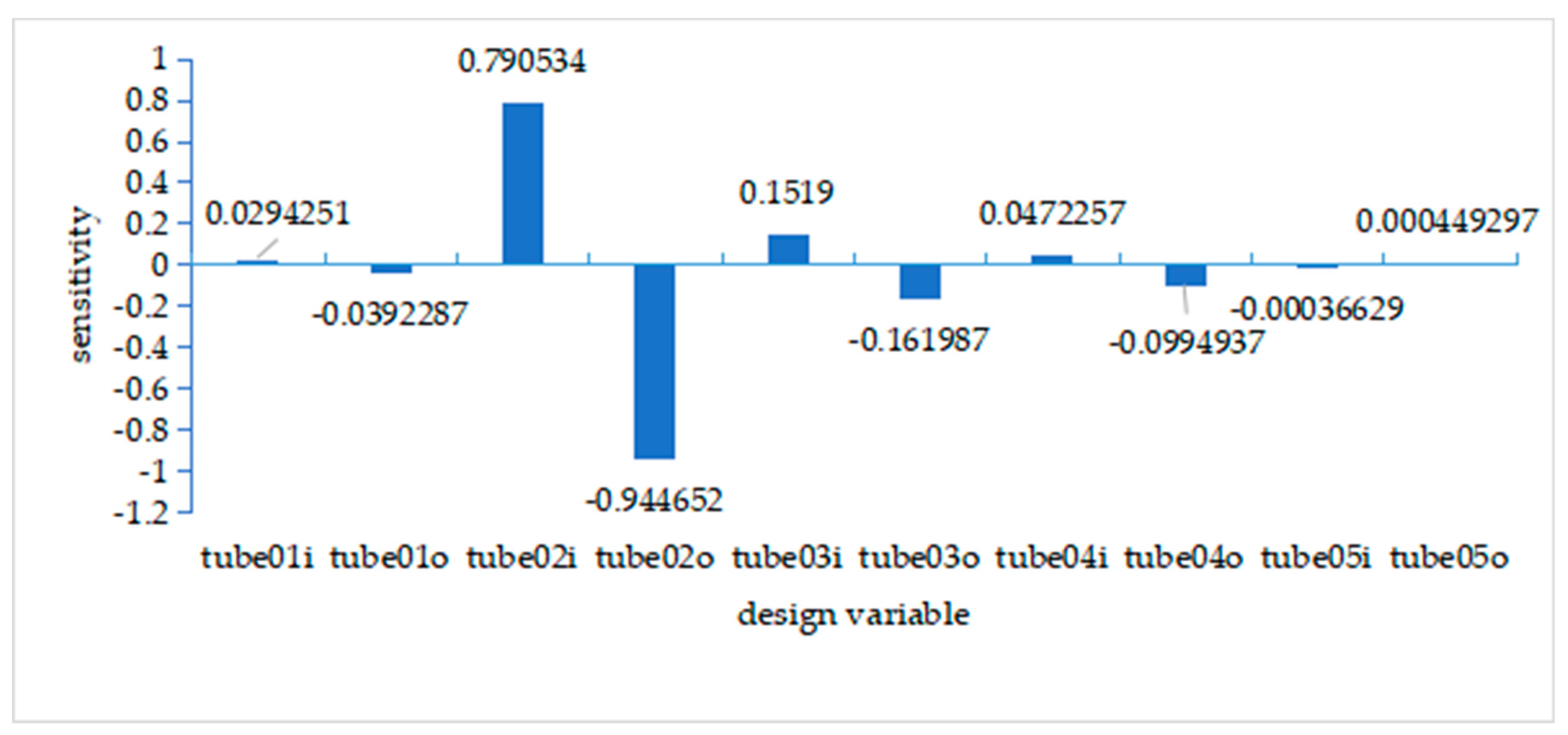
Considering that the residual stress under each working condition is relatively large, size optimization mainly focuses on the direction of strain. After post-processing the visualization file in HyperGraph, the sensitivity analysis results are shown in Figure 17. Except for the first five pipe fittings, the sensitivity of other pipe fittings is very low and can be ignored. The sensitivity is positive, indicating that the calculated variables and factors change in a positive direction. When the sensitivity is negative, it indicates that the calculated variable changes in the opposite direction from the factor.
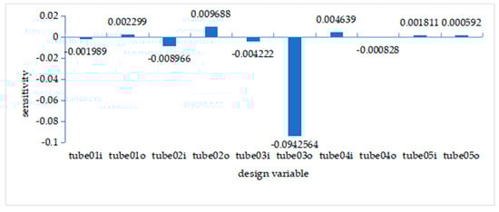
Figure 17.
Quality sensitivity.
On the premise of meeting the strength requirements, the second pipe fitting has the greatest impact on the overall quality of the vehicle. However, due to the basic determination of the hard point position of the suspension, it is considered necessary to adjust the side collision avoidance structure.
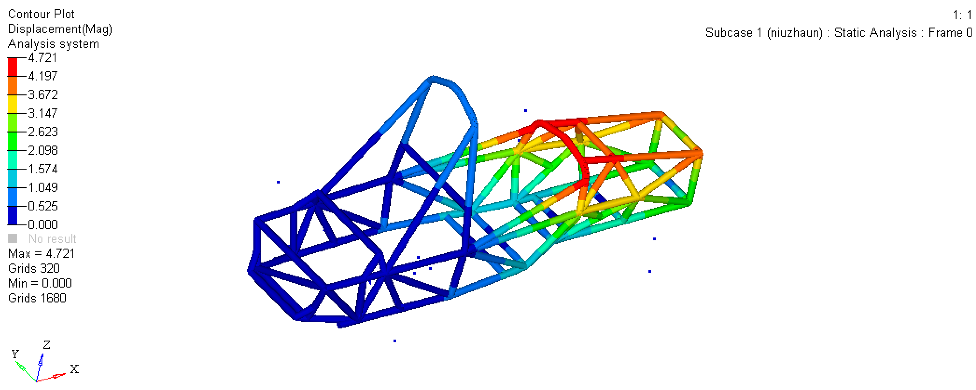
Analysis of Figure 18, Figure 19 and Figure 20 reveals that the maximum strain values under bending, braking, and turning conditions primarily occur near the bottom of the cabin. Overall, the No. 2 and No. 3 pipe fittings have a relatively significant influence. Therefore, adjusting the structure of the cabin can effectively reduce the deformation of the pipe fittings. The next design focus is to decrease the wall thickness of the pipe fittings in this area. Table 3 presents the data for some pipe fittings after the solution. The outer diameter of the steel tube is set to 25.4 mm. To ensure that the wall thickness of the steel tube does not exceed 2 mm, the inner diameter is set to 23.4 mm. From the sensitivity results obtained in Figure 17, Figure 18, Figure 19 and Figure 20, it can be observed that the sensitivity is nearly 0 for steel pipe numbered 5, indicating that it has little effect on the overall frame. As a result, it can be ignored. After optimization, both the inner and outer diameters of the steel pipe will change. To comply with the competition’s specified standard of an outer diameter not exceeding 25.4 mm and the actual steel pipe specifications, the optimized inner and outer diameters should be adjusted accordingly. Finally, the frame is designed based on the corrected inner and outer diameters to ensure compliance with specifications.
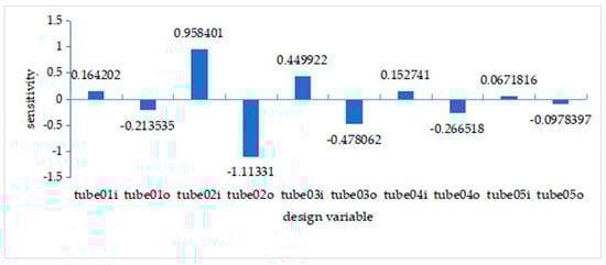
Figure 18.
Strain sensitivity under bending conditions.

Figure 19.
Strain sensitivity under emergency braking conditions.
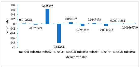
Figure 20.
Strain sensitivity under high-speed turning conditions.
Table 3.
Optimization results of the pipe size for part of the frame.
3.3.4. Comparison between the Optimized Frame and the Original Frame
- (1)
- Quality change: After size optimization, according to the results of sensitivity analysis, Table 2 shows that the diameter of No.2 and No.3 pipe fittings changes greatly; that is, the wall thickness of steel pipe decreases. In the solution report, the weight of the frame is reduced from 45.71 kg to 39.87 kg, which is reduced by 12.8%;
- (2)
- Strength change: As shown in Table 4, compared with the existing frame, the maximum displacement and maximum stress of the original frame have decreased to varying degrees under various working conditions, the strength performance has improved, and the modal has also been correspondingly improved;
Table 4. Strength comparison before and after optimization.
- (3)
- Stiffness comparison: As shown in Figure 21, a force of 2000 N was applied to the optimized model under torsion conditions, resulting in a torsion angle of 0.592°. According to the formula K = T/θ, the calculated stiffness is 1718.3 Nm/°, which increases by 16.7% compared to the original torsional stiffness calculated in Section 2.4.2;
 Figure 21. Optimized torsional stiffness related data.
 - (4)
- Modal comparison: The lowest-order modal of the frame increases by 0.75 Hz, which improves the handling stability and driving safety of the vehicle.
Based on the above analysis, the overall performance of the optimized frame has been improved, thus meeting the requirements of lightweight design.
4. Conclusions
The main contribution of this paper lies in the integration of two methods for frame design optimization. Firstly, we propose a global topology optimization approach based on the variable density method to comprehensively solve the frame and obtain an accurate material distribution solution. Secondly, we introduce sensitivity analysis utilizing the adjoint variable method to identify the influential factors of design variables within the racing frame context. Based on the magnitude of these influence factors, optimal design variables are determined, and the frame size is subsequently optimized to reduce its weight and refine its structure. Finally, a performance comparison is conducted between the current frame and the original frame to validate the feasibility of the optimized design.
However, it is worth noting that the topology optimization method based on the variable density method is considered outdated as it involves a time-consuming post-processing stage. In this era of intelligence, there is hope for the future introduction of optimization design techniques based on deep learning into the field of racing frame design.
Author Contributions
Conceptualization, W.M., Y.L., P.W., Y.W. and J.W. All authors have read and agreed to the published version of the manuscript.
Funding
This research received no external funding.
Conflicts of Interest
The authors declare no conflict of interest.
References
- Hetawal, S.; Gophane, M.; Ajayb, K. Aerodynamic study of formula FSAE car. Procedia Eng. 2016, 97, 1198–1207. [Google Scholar] [CrossRef]
- Song, S. Joint Study on Aerodynamics and Handling Stability of FSAE Racing Car under Unsteady Wind; Jilin University: Changchun, China, 2021. [Google Scholar]
- Ni, J.; Bin, X. Modeling and handling stability simulation of FSAE racing car based on ADAMS. Eng. Des. J. 2019, 18, 354–358. [Google Scholar]
- Vaidya, S.; Kulkarni, C. Aerodynamic development of a formula FSAE car: Initial Design Stage. Int. J. Eng. Res. Technol. 2017, 6, 14–18. [Google Scholar]
- Gui, C.; Bai, J.; Zuo, W. Simplified crash worthiness method of automotive frame for conceptual design. Thin-Walled Struct. 2018, 131, 324–335. [Google Scholar] [CrossRef]
- Yu, H.; Xu, H.; Zhou, C. Optimization of single shell body of composite material for Formula Student Racing. J. Tongji Univ. Nat. Sci. Ed. 2016, 44, 1729–1734. [Google Scholar]
- Hu, L.; Shi, Y.; Yang, Q. Optimization design of a certain type of college students’ formula racing car frame based on finite element method. J. Wuhan Univ. Sci. Technol. Nat. Sci. Ed. 2017, 38, 31–34. [Google Scholar]
- Kong, D.; Li, W.; Xiao, X. Lightweight design of Formula Racing Frame. Mech. Des. 2021, 26, 455–459. [Google Scholar]
- Abdi, M.; Ashcroft, I.; Wildman, R. Topology optimization of geometrically nonlinear structures using an evolutionary optimization method. Eng. Optim. 2018, 50, 1850–1870. [Google Scholar] [CrossRef]
- Chen, Y.; Gao, L.; Xiao, M. Topology optimization design of heat dissipation structure based on variable density method. Comput. Integr. Manuf. Syst. 2018, 24, 117–126. [Google Scholar]
- Zhu, B.; Chen, Q.; Wang, R. Structural topology optimization using a moving morph able component-based method considering geometrical non-linearity. J. Mech. Des. 2018, 140, 081403. [Google Scholar] [CrossRef]
- Zang, J.; Peng, Y.; Liu, M. Topology optimization design of continuum structures based on multi-performance constraints. Comput. Integr. Manuf. Syst. 2022, 28, 1746. [Google Scholar]
- Jung, T.; Lee, J.; Nomura, T.; Dede, E. Inverse design of three-dimensional fiber reinforced composites with spatially-varying fiber size and orientation using multiscale topology optimization. Compos. Struct. 2022, 279, 114768. [Google Scholar] [CrossRef]
- Zhao, F. A nodal variable ESO (BESO) method for structural topology optimization. Finite Elem. Anal. Des. 2019, 86, 34–40. [Google Scholar] [CrossRef]
- Xie, L.; Zhang, Y.; Ge, M. Topology optimization of heat sink based on variable density method. Energy Rep. 2022, 8, 718–726. [Google Scholar] [CrossRef]
- Christensen, J.; Bastien, C. Introduction to structural optimization and its potential for development of vehicle safety structures. In Book: Nonlinear Optimization of Vehicle Safety Structures; Butterworth-Heinemann: Oxford, UK, 2019; pp. 169–207. [Google Scholar]
- Rodriguez, T.; Montemurro, M.; Texier, P.; Pailhès, J. Structural displacement requirement in a topology optimization algorithm based on isogeometric entities. J. Optim. Theory Appl. 2020, 184, 250–276. [Google Scholar] [CrossRef]
- Smith, H.; Norato, J. A MATLAB code for topology optimization using the geometry projection method. Struct. Multidiscip. Optim. 2020, 62, 1579–1594. [Google Scholar] [CrossRef]
- Zhang, W.; Jiang, Q.; Feng, W.; Youn, S.; Guo, X. Explicit structural topology optimization using boundary element method-based moving morphable void approach. Int. J. Numer. Methods Eng. 2021, 122, 6155–6179. [Google Scholar] [CrossRef]
- Lu, J.; Ding, J. Direct differential method for sensitivity analysis of multibody system dynamics design. J. Qingdao Univ. Eng. Technol. Ed. 2019, 19, 76–79. [Google Scholar]
- Blondel, M.; Berthet, Q.; Cuturi, M. Efficient and modular implicit differentiation. Adv. Neural Inf. Process. Syst. 2022, 35, 5230–5242. [Google Scholar]
- Wang, B.; Yuan, Z.; Hu, J.; Yao, W. Simulation Analysis and Experimental Study of Baja Racing Car Frame Based on Special Working Conditions. SAE Technical Paper 2023, 214–232. [Google Scholar]
- Lyduch, K.; Szymanski, S.; Nowak, M. The frame design of a three-wheeled vehicle for a student competition using topology optimization. Int. J. Interact. Des. Manuf. 2022, 16, 927–942. [Google Scholar] [CrossRef]
- Fu, S.; Li, Y.; Xiong, X.; Hu, L.; Jun, H.; Zhou, S. Optimal design of the frame of baja racing car for college students. In Proceedings of the China SAE Congress 2020: Selected Papers, Shanghai, China, 27–29 October 2022; pp. 293–310. [Google Scholar]
- Krzikalla, D.; Sliva, A.; Petru, J. On modelling of simulation model for racing car frame torsional stiffness analysis. Alex. Eng. J. 2020, 59, 5123–5133. [Google Scholar] [CrossRef]
- Napolitano, G.; Adiletta, G.; Farroni, F.; Sakhnevych, A.; Timpone, F. Tire wear sensitivity analysis and modeling based on a statistical multidisciplinary approach for high-performance vehicles. Lubricants 2023, 11, 269. [Google Scholar] [CrossRef]
- He, Y.; Pang, J. Optimization design of suspension geometric parameters of formula student race vehicle based on ADAMS. In Proceedings of the 2022 International Conference on Manufacturing, Industrial Automation and Electronics (ICMIAE), Rimini, Italy, 26–28 August 2022; pp. 164–169. [Google Scholar]
- Plante, E.; Bideaux, E.; Delhommais, M.; Gerard, M. Large size optimization problem for power management in a fuel cell electric race car using combinatorial approach. In Proceedings of the IECON 2022–48th Annual Conference of the IEEE Industrial Electronics Society, Brussels, Belgium, 17–20 October 2022; pp. 125–138. [Google Scholar]
- Jang, W. Optimal design for torsional stiffness of the tubular space frame of a low-cost single seat race Car. J. Korea Acad.-Ind. Coop. Soc. 2021, 15, 5955–5962. [Google Scholar]
- Yuan, S.; Lin, J. Design and lightweight of FSAE racing car frame. J. Zhengzhou Univ. (Eng. Ed.) 2018, 39, 18–24. [Google Scholar]
- Chen, H.; Lu, C.; Liu, Z. Structural modal analysis and optimization of SUV door based on response surface method. Shock Vib. 2020, 185–206. [Google Scholar] [CrossRef]
- Li, K.; Cheng, G. Structural topology optimization of elastoplastic continuous under shakedown theory. Int. J. Numer. Methods Eng. 2022, 123, 4459–4482. [Google Scholar] [CrossRef]
- Xu, S.; Liu, J.; Zou, B. Stress constrained multi-material topology optimization with the ordered SIMP method. Comput. Methods Appl. Mech. Eng. 2021, 373, 113453. [Google Scholar] [CrossRef]
- Kijanski, W.; Barthold, F. Two-scale shape optimisation based on numerical homogenisation techniques and variational sensitivity analysis. Comput. Mech. 2021, 67, 1021–1040. [Google Scholar] [CrossRef]
- Chun, J. Reliability-Based design optimization of structures using complex-step approximation with sensitivity analysis. Appl. Sci. 2021, 11, 4708. [Google Scholar] [CrossRef]


Disclaimer/Publisher’s Note: The statements, opinions and data contained in all publications are solely those of the individual author(s) and contributor(s) and not of MDPI and/or the editor(s). MDPI and/or the editor(s) disclaim responsibility for any injury to people or property resulting from any ideas, methods, instructions or products referred to in the content. |
© 2023 by the authors. Licensee MDPI, Basel, Switzerland. This article is an open access article distributed under the terms and conditions of the Creative Commons Attribution (CC BY) license (https://creativecommons.org/licenses/by/4.0/).