Computer Vision Based Planogram Compliance Evaluation

Abstract

Arranging products in stores according to planograms, optimized product arrangement maps, is an important sales enabler and necessary for keeping up with the highly competitive modern retail market. Key benefits of planograms include increased efficiency, maximized retail store space, increased customer satisfaction, visual appeal, and increased revenue. The planograms are realized into product arrangements by humans, a process that is prone to mistakes. Therefore, for optimal merchandising performance, the planogram compliance of the arrangements needs to be evaluated from time to time. We investigate utilizing a computer vision problem setting—retail product detection—to automate planogram compliance evaluation. Retail product detection comprises product detection and classification. The detected and classified products can be compared to the planogram in order to evaluate compliance. In this paper, we propose a novel retail product detection pipeline combining a Gaussian layer network product proposal generator and domain invariant hierarchical embedding (DIHE) classifier. We utilize the detection pipeline with RANSAC pose estimation for planogram compliance evaluation. As the existing metrics for evaluating the planogram compliance evaluation performance assume unrealistically that the test image matches the planogram, we propose a novel metric, called normalized planogram compliance error $\left(E_{PC}\right)$, for benchmarking real-world setups. We evaluate the performance of our method with two datasets: the only open-source dataset with planogram evaluation data, GP-180, and our own dataset collected from a large Nordic retailer. Based on the evaluation, our method provides an improved planogram compliance evaluation pipeline, with accurate product location estimation when using real-life images that include entire shelves, unlike previous research that has only used images with few products. Our analysis also demonstrates that our method requires less processing time than the state-of-the-art compliance evaluation methods.

1. Introduction

In the modern, highly competitive retail environment, work efficiency is essential and requires algorithmic optimization of operations. This includes optimization of the display and arrangement of products in stores: planograms, charts that show where each product should reside on a shelf, are often generated by specialized software, and the products are then arranged accordingly. Studies have shown that complying with optimized planograms can increase sales up to 7–8%, and that the total cost of suboptimal merchandising sales performance in the US is approximately 1% of gross product sales [1]. Over 60 percent of purchase decisions are made at the point of sale for which visibility and presentation, and thereby decisions made through a planogram, are vital for motivating sales.

As the planograms are “realized” into product arrangements by people, the possibility of human error is always present. Therefore, the arrangements need to be checked for planogram compliance—whether the arrangement of products in-store truly matches the desired arrangement given by the planogram—from time to time. This, too, is still a manual task, requiring costly human resources. Computers, on the other hand, have better memories, do not make mathematical errors, and are better at multitasking than humans, and therefore a computer-based compliance method is appealing. We encourage the reader who is less familiar with the latest deep learning-based methods of computer vision to look for background information from the field’s foundational sources [2,3].

Object detection is a computer vision task that could provide automation for planogram compliance evaluation. Most object detection literature deals with generic object detection—recognizing everyday objects in everyday environments. This includes approaches such as feature pyramid networks (FPNs) [4], region-based convolutional neural networks (R-CNNs) [5], and you only look once (YOLO) [6], as well as challenges such as ImageNet [7] and MS COCO [8]. However, recognizing retail products in the environment of racks is a mix of generic object detection and object instance detection. Object instance detection means detecting a specific object instead of a general class, as is carried out in general object detection. In the retail product detection problem setting, the aim is to localize and classify products from images of shelves, cabinets, racks, or bays taken in retail store aisles. The recognition process is called the retail product detection problem [9], and it exhibits a number of difficulties in comparison to this more general problem that has made using computer vision for planogram compliance verification infeasible for quite some time.

The two most fundamental difficulties of retail product detection—the small amount of available training data per class and the domain shift between training data and test data—were identified already by [10], who kick-started research into retail product detection in 2007. Other difficulties of retail product detection when compared to generic object detection and object instance detection include the very high number of object classes (in the order of several thousand for small shops and tens of thousands for hypermarkets); the closeness of the appearance of the object classes (for example, for different flavors of the same product from the same brand), requiring fine-grained classification; and the frequently changing assortment-making models that require slow retraining infeasible [11]. Due to these peculiarities, the results achieved by [10]—and, indeed, results achieved with any pure generic object detection or instance detection methods—were quite poor.

Retail product detection approaches that perform well enough to be utilized in practice have emerged only recently. Local invariant feature-based approaches have been utilized to solve the problem well beyond the breakthrough of CNNs for generic object detection. Notable approaches that utilize invariant features, in addition to the seminal [10], include combining corner detection, color information, and Bag of Words [12]; utilizing BRISK features and Hough transform estimation [13]; and detecting products one shelf level at a time with SURF features and dimensionality information-based refinement [14].

The first papers discussing the use of deep learning for retail product detection were published only in 2017. Initially, deep learning was utilized in hybrid approaches, that is, in combination with local invariant features. In notable hybrid models, deep learning was used for product classification [12] showing the power of deep learning over more traditional methods in the case of complex (that is, realistic) scenarios and [15] presenting a non-parametric probabilistic model for initial detection with CNN-based refinement trying to overcome the lack of training data. An attention mechanism was added by Geng et al. [16], improving the detection accuracy and adaptability to new product classes without retraining.

Starting in 2018, fully deep-learning-based product detection pipelines have started to emerge. These include combining a class-agnostic object detector with an encoder network utilized for classification into a model that, after being trained once, was able to fit new stores, products, and packages of existing products [11] and combining RCNN [5] object detection and ResNet-101 [17] classification with a specialized non-maximal suppression approach for rejecting region proposals for unlikely objects arising from overlapping products in images [18].

In addition to end-to-end retail product detection, research has been carried out towards product proposal generation—detecting the objects without classifying them. The main obstacle with this research was, until 2019, the lack of quality training data, with attempts to circumvent this via, e.g., 3-D renderings [19]. In 2019, however, Ref. [20] introduced the SKU-110K dataset, including images collected from thousands of supermarket stores and being of various scales, viewing angles, lighting conditions, and noise levels and thus enabled the training of deep product proposal generators. The baseline product proposal generation approach of [20] consisted of combining RetinaNet with a Gaussian-based non-maximal suppression. Later utilizations of SKU-110K include baking the Gaussian non-maximal suppression into the product proposal generator network itself, thus resulting in a multi-task learning problem [21], and addressing object rotations and outlier training samples with engineered-for-purpose neural network models [22].

The other end of end-to-end retail product detection—that is, retail product classification—has also seen some research separate from the full problem. One notable approach is that of [23], which combines training an encoder for k-nearest neighbor (KNN) product classification with utilizing generative adversarial networks (GANs) for data augmentation and a distance measure that takes into account the product hierarchy.

The planogram compliance evaluation problem is not solved by just detecting the products. Additionally, the detected arrangement needs to be compared to the planogram, and any deviations noted. This is not trivial, either: the exact positions where the products given in the planogram should be in the image are rarely known.

Planogram compliance evaluation is not as well researched as retail product detection. The seminal articles [1,24] came out in 2015, with approaches consisting of the utilization of detecting subsections of shelves [1] and distance metrics of the current shelf image with an image of the shelf taken in its ideal, planogram-compliant state [24]. Other notable approaches to the problem include viewing it as a recurring pattern detection problem [25], evaluating compliance one shelf at a time with the help of directed acyclic graphs (DAGs) [14], and viewing the product arrangements as graphs and solving for a maximum common subgraph between them [13]. The evaluation methods used in existing research on planogram compliance evaluation seem to assume that the test images match the planograms and to then just calculate standard object detection performance metrics based on how many of the facings were indeed detected. We argue that for a real-world use case, having test images that do not fully match the planogram is more interesting than having only a hundred percent compliant images. To enable evaluating planogram compliance evaluation methods with datasets that correct this deficiency, we propose a novel metric called normalized planogram compliance error $E_{PC}$.

Some of the recent developments bordering retail product detection have not been to our knowledge yet utilized in a full retail product detection pipeline. On the one hand, the SKU-110K dataset [20] has enabled the training of product proposal generators, deep neural networks that locate the products without classifying them, on an unprecedented scale. The dataset has already been successfully utilized in networks such as the Gaussian layer network (GLN) [21] and the dynamic refinement network [22]. On the other hand, the domain invariant hierarchical embedding (DIHE) [23] introduced the idea of utilizing GANs to train an encoder for KNN classification to be used for product classification purposes.

To enable planogram compliance evaluation on large, real-world shelves and to take planogram compliance evaluation to the neural network era, we propose a novel retail product detection pipeline using GLN for product detection, DIHE for product classification, and RANSAC for pose estimation [26]. Our proposed pipeline is suitable for use in all brick-and-mortar stores regardless of the retail vertical. As the conventional metrics used for evaluating the performance of object detection are not suitable for planogram compliance detection, we propose a novel metric. We summarize our main contributions as follows:

• We propose a novel retail product detection pipeline by combining a product proposal generator [21] with a product classification approach [23], and compare the product proposal generation, product classification, and retail product detection performance of the resulting framework to existing approaches.
• We utilize the product detection pipeline and RANSAC pose estimation [26] to evaluate planogram compliance on real retail data consisting of full planograms and images that are not fully planogram compliant, while previous research has focused on small fully compliant subsections of planograms
• We propose a novel metric, the mean-squared planogram compliance error, for benchmarking planogram compliance detection performance.

2. Materials and Methods

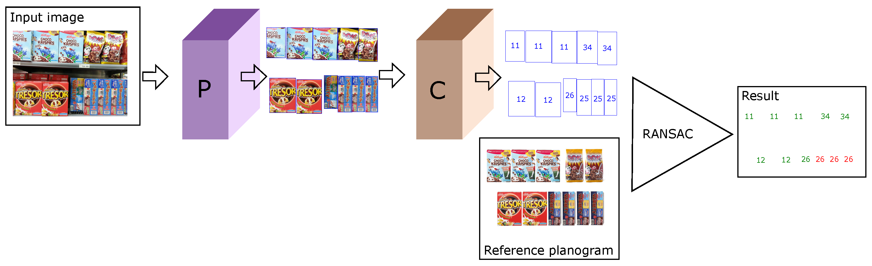
Our proposed approach consists of a two-stage product detector and a RANSAC comparison between the planogram and the detections. We choose a two-stage detector over a one-stage one due to a number of reasons related to the retail product detection problem: one-stage approaches need retraining whenever the assortment changes; one-stage detectors have been shown to fare poorly against two-stage approaches when dealing with a multitude of small objects, which is a common scenario in retail product detection [27]; and a two-stage detector allows us to choose and improve upon both of the components separately.

The proposed two-stage detector utilizes a deep product proposal generator [21] as its first stage, and classifies these proposals with an encoder-based approach [23] in the second stage. The first stage is selected due to its impressive performance with the SKU-110K dataset, which leads us to expect top-level performance in real-world use. The second stage is selected for its novel way of dealing with the domain shift, its ability to handle an arbitrary amount of classes, and its ability to classify products that were not present in the training data.

The detector outputs an empirical planogram, which is then compared to the expected planogram utilizing RANSAC-based pose estimation. The approach is visualized in Figure 1.

2.1. Product Proposal Generation

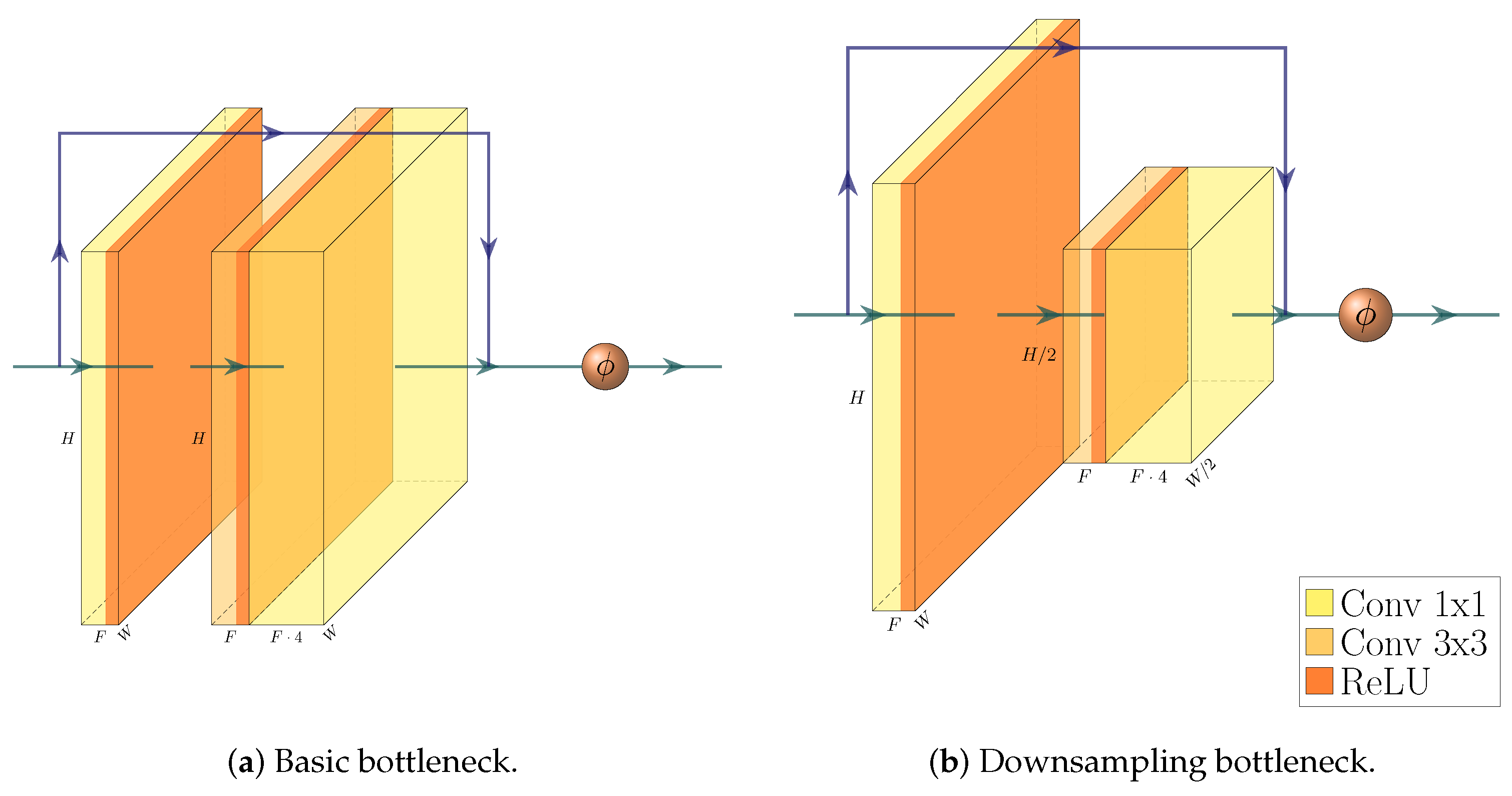
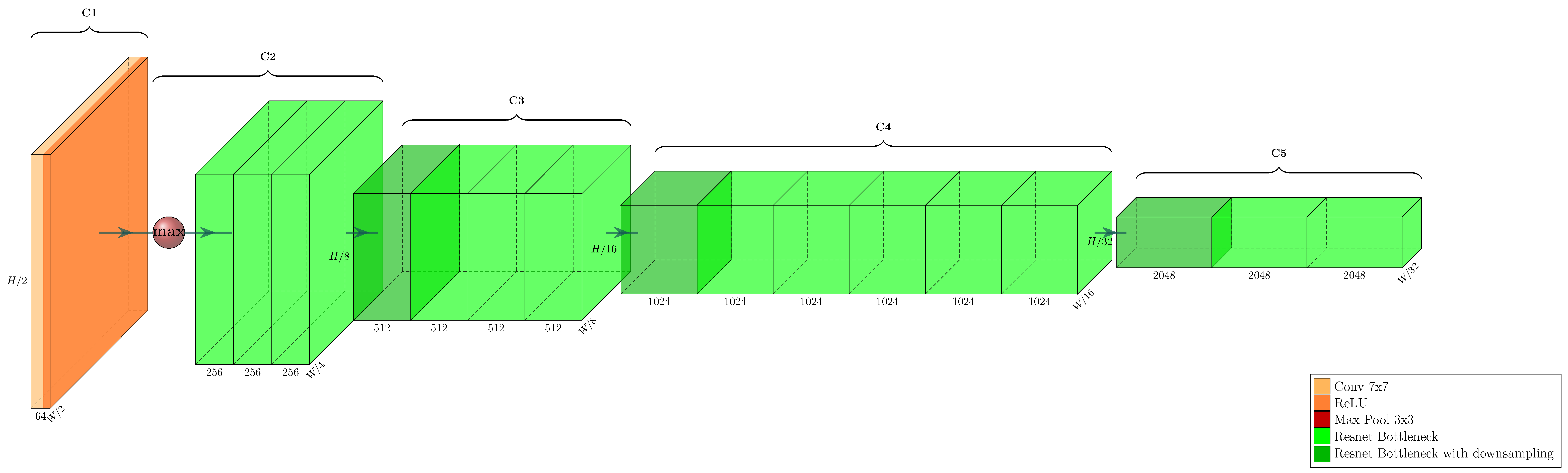
We follow the example of [21] in choosing ResNet-50, a fully convolutional object classification network, pre-trained with the ImageNet dataset [7], as the backbone for our product proposal generator. The backbone architecture is visualized in Figure 2 and Figure 3.

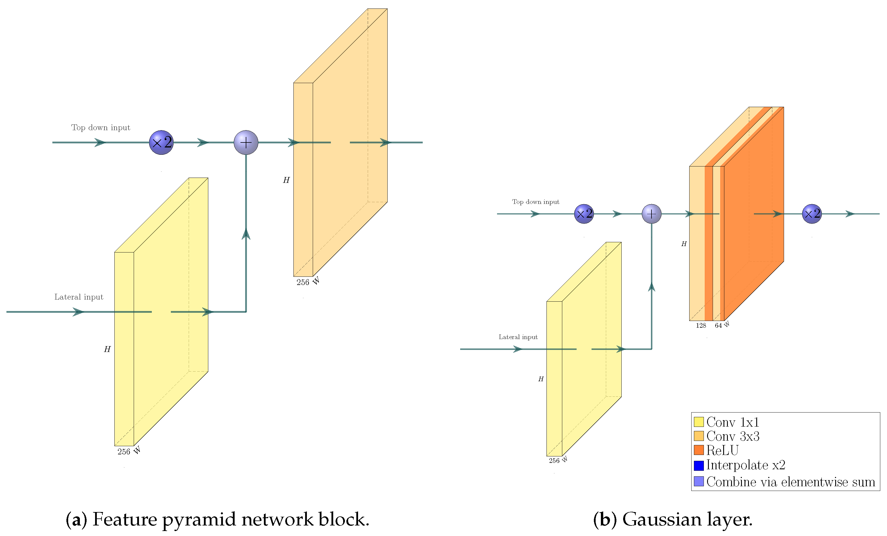
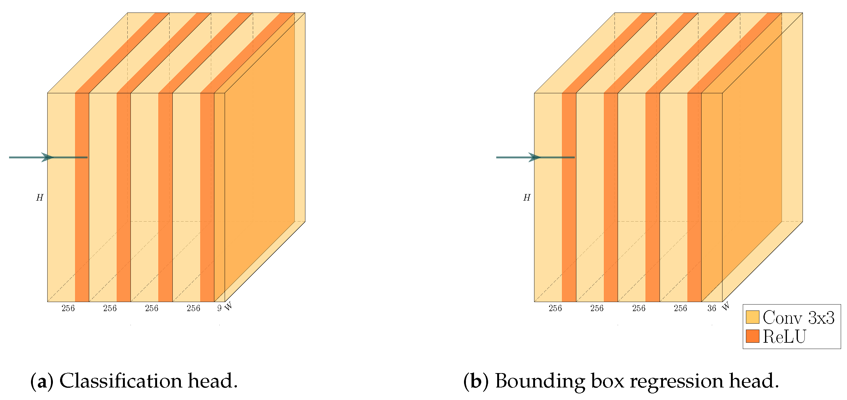
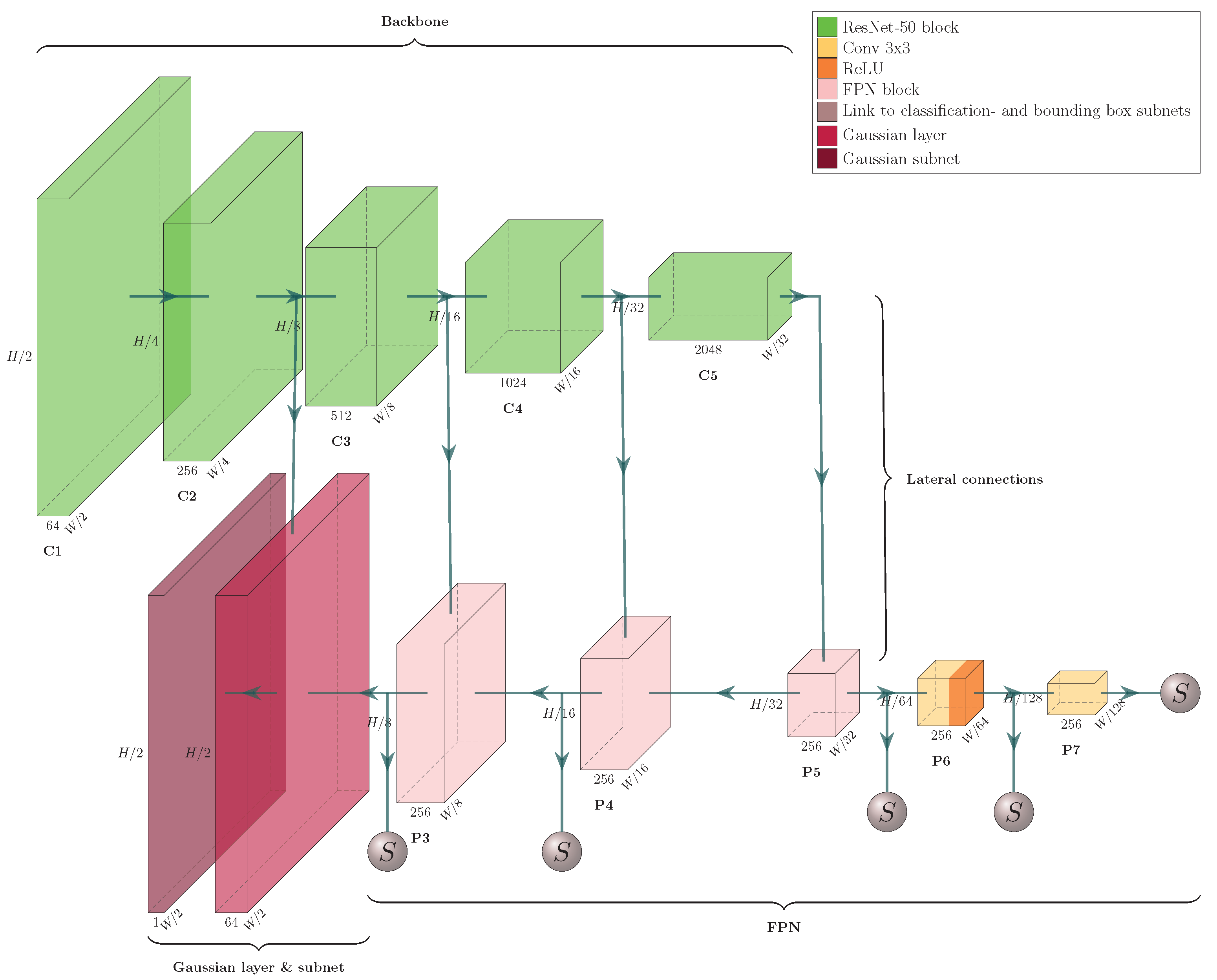
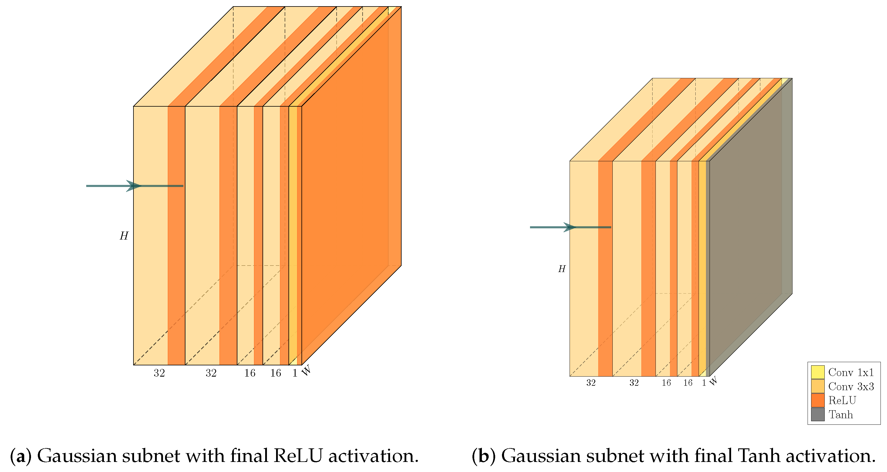
We build a feature pyramid network (FPN, Ref. [4]) on top of this backbone, and augment the architecture further by making our network training a multi-task learning problem via the introduction of a Gaussian layer and subnet [21]. The architecture of the resulting network is visualized in Figure 4, Figure 5, Figure 6 and Figure 7. We further explore substituting the ReLU activation of the final layer of the Gaussian subnet with Tanh. Our intuition here is that as the prediction target of the Gaussian subnet is limited to the range $[0,1]$, it makes sense to bar the neural network from producing values outside of this range. This alternative is visualized in Figure 6b.

As suggested by [21], we use a weighted sum of three different loss functions, each calculated from different outputs of our product proposal generator network. Our full loss function is

$$\mathcal{L}={\alpha }_{\mathrm{focal}}{\mathcal{L}}_{\mathrm{focal}}+{\mathcal{L}}_{L_1}+{\alpha }_{\mathrm{MSE}}{\mathcal{L}}_{\mathrm{MSE}}.$$

(1)

In the above equation, ${\mathcal{L}}_{\mathrm{focal}}$ is focal loss [30]. We use it for foreground–background classification loss. It is calculated as

$${\mathcal{L}}_{\mathrm{focal}}\left(p_t\right)=-{\alpha }_t{(1-p_t)}^{\gamma }log\left(p_t\right),$$

(2)

where

$${\alpha }_t=\left\{\begin{array}{cc}\alpha \hfill & \mathrm{if}\mathrm{the}\mathrm{detection}\mathrm{belongs}\mathrm{to}\mathrm{the}\mathrm{foreground},\hfill \\ 1-\alpha \hfill & \mathrm{otherwise}\hfill \end{array}\right..$$

(3)

$\alpha \in [0,1],\gamma \ge 0$ are hyperparameters,

$$p_t=\left\{\begin{array}{cc}p\hfill & \mathrm{if}\mathrm{the}\mathrm{detection}\mathrm{belongs}\mathrm{to}\mathrm{the}\mathrm{foreground},\hfill \\ 1-p\hfill & \mathrm{otherwise}\hfill \end{array}\right.,$$

(4)

and $p\in [0,1]$ is the estimated probability that the detection belongs to the foreground [30].

${\mathcal{L}}_{L_1}$ is $L_1$ loss, or, in other words, mean absolute error. We use it as our bounding box regression loss. It is defined as

$${\mathcal{L}}_{L_1}(x,\widehat{x})=|x-\widehat{x}|,$$

(5)

where x is the ground truth, and $\widehat{x}$ is the prediction.

Finally, ${\mathcal{L}}_{\mathrm{MSE}}$ is the mean-squared error. It is used as the loss for our multi-task learning part—the loss between our generated Gaussian maps and ground-truth Gaussian maps. It is calculated as

$${\mathcal{L}}_{MSE}(x,\widehat{x})={(x-\widehat{x})}^2,$$

(6)

where x is the ground-truth Gaussian map, and $\widehat{x}$ is the prediction. The Gaussian loss is only calculated for coordinates where x is either 0 or larger than a hyperparameter, $\omega$ [21].

${\alpha }_{\mathrm{focal}}$ and ${\alpha }_{\mathrm{MSE}}$ are weighting parameters for focal loss and MSE, respectively. We use them to tune the loss function in order to achieve more stable training and better results.

2.2. Product Classification

We use an embedding approach, the domain invariant hierarchical embedding (DIHE, Ref. [23]), as our product classification model. It consists of three networks: the encoder, the generator, and the discriminator.

The encoder network learns an embedding, and a function from images into vectors, with the distance between two output vectors signifying the similarity between the respective images. This embedding can be used to classify images via nearest neighbor search: the query image is converted into a vector with the encoder, and it is assigned a class based on the nearest embedding of a reference image. The encoder is the only network that is used beyond the training stage.

The generator and discriminator are only used to augment the data when training the encoder. The purpose of this is to overcome the lack of data inherent with retail product image sets and to combat the problems caused by domain shift, that is, the training images being clear and iconic while the test images are noisy crops from an image of a retail store shelf.

We selected the VGG16 [31] as the encoder network pre-trained with ImageNet, following the example of [23]. We use maximum activation of convolutions (MACs)—the maximum value produced by select convolution layers—as the output of our encoder network, due to [23] achieving their best results with this approach. The encoder architecture is visualized in Figure 8.

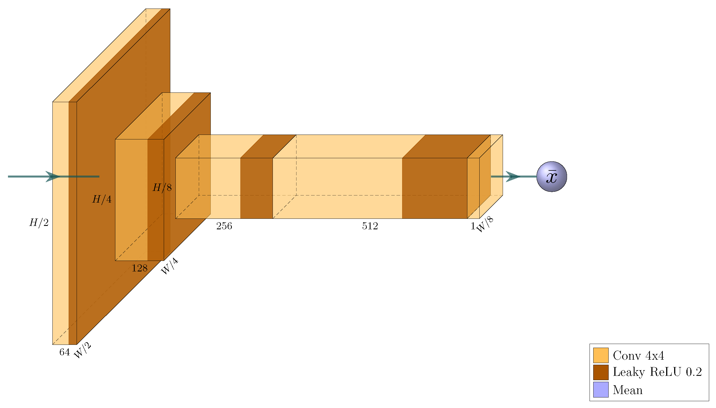
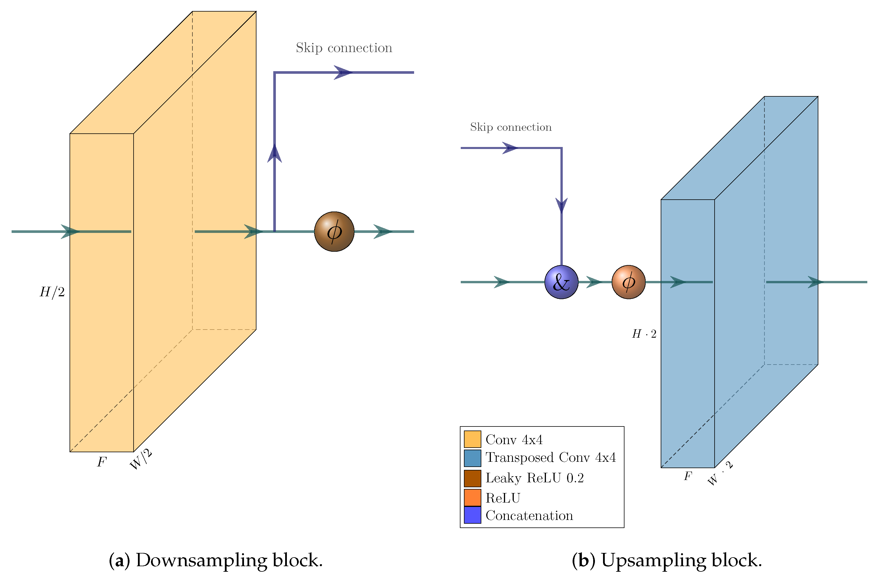
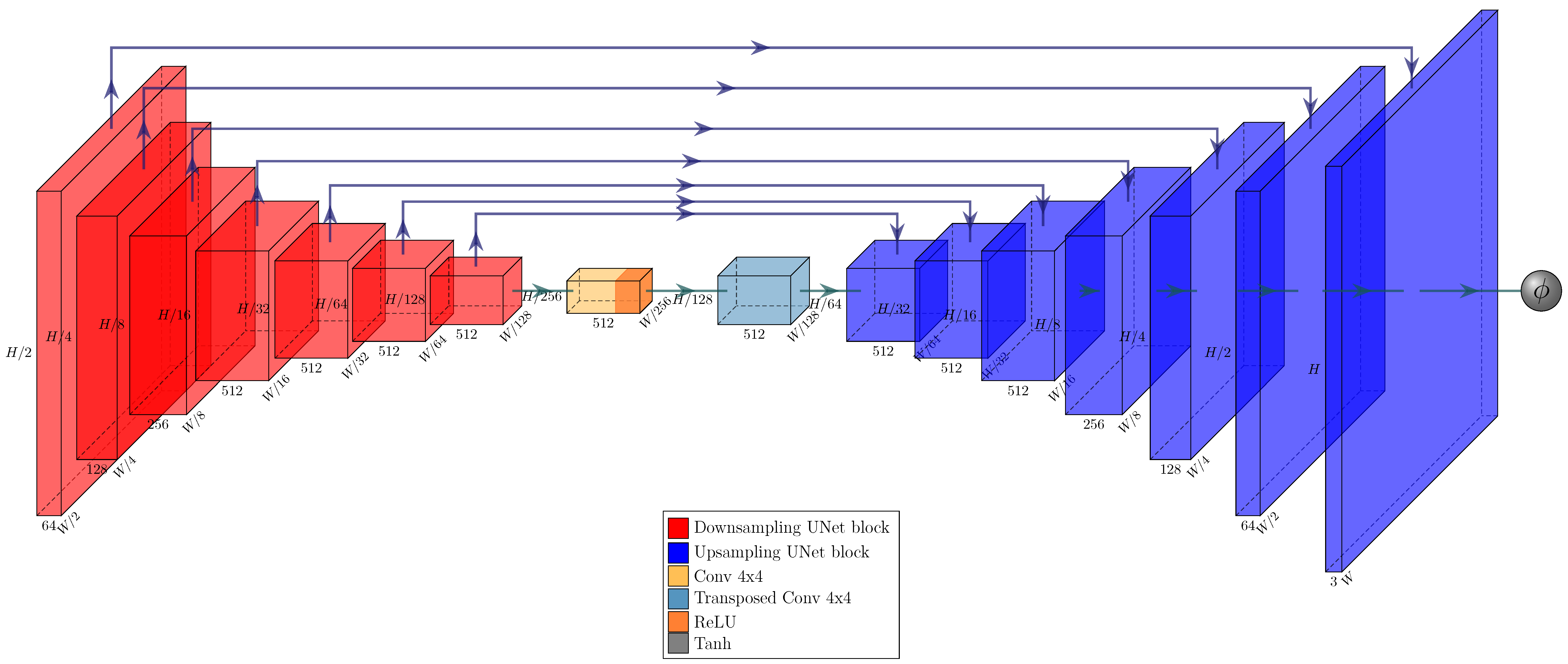
For the generator and discriminator, we adopt the pix2pix GAN, Ref. [32] again, following the example of [23]. The GAN architecture is visualized in Figure 9, Figure 10 and Figure 11.

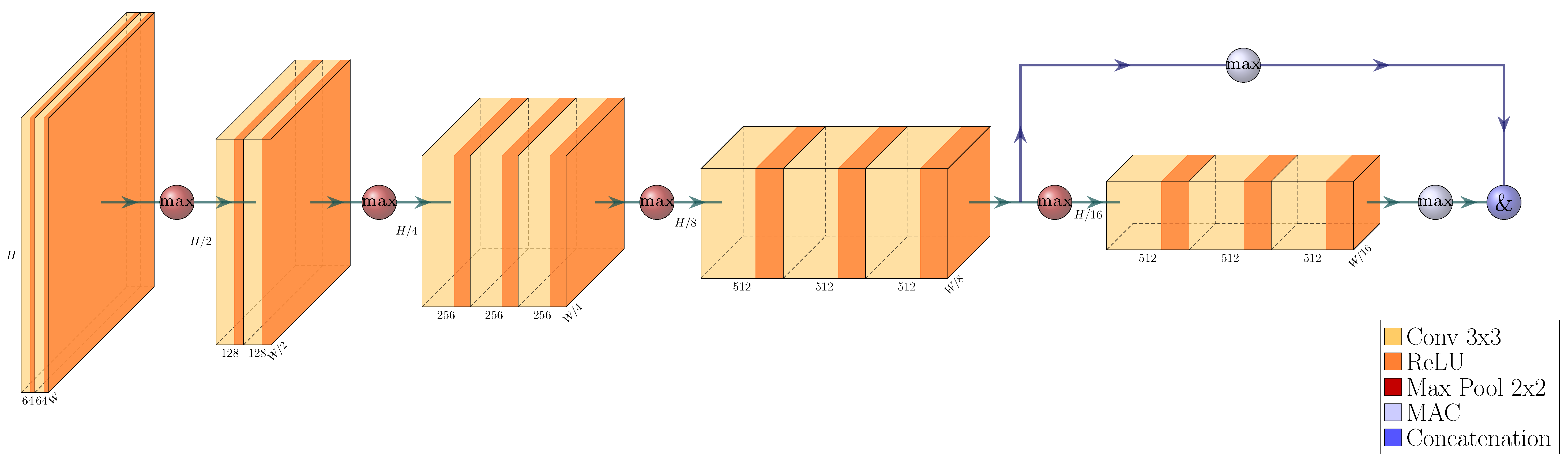
Figure 8. VGG16 encoder utilizing MAC descriptors, built from the PyTorch implementation of said network [29,31,33]. The input is an image with shape $3\times H\times W$. The model outputs a 1024-element MAC descriptor, with the first 512 elements determined by the maximum activations of the last layer of the second-to-last convolutional block, and the remaining 512 elements determined by the maximum activations of the last convolution layer. Downsampling is implemented via stride 2 when max pooling.

Figure 8. VGG16 encoder utilizing MAC descriptors, built from the PyTorch implementation of said network [29,31,33]. The input is an image with shape $3\times H\times W$. The model outputs a 1024-element MAC descriptor, with the first 512 elements determined by the maximum activations of the last layer of the second-to-last convolutional block, and the remaining 512 elements determined by the maximum activations of the last convolution layer. Downsampling is implemented via stride 2 when max pooling.

Keeping with the methodology of [23], we use domain invariant hierarchical embedding loss (${\mathcal{L}}_{\mathrm{DIHE}}$) to train our encoder:

$${\mathcal{L}}_{\mathrm{DIHE}}(i_p,i_n,h_p,h_n)={\mathcal{L}}_{\mathrm{triplet}}(G\left(i_p\right),i_p,i_n,{\alpha }_{\mathrm{hierarchial}}(h_p,h_n)),$$

(7)

where $i_p$ is an image belonging to the class of interest, $i_n$ an image belonging to a different (randomly drawn) class, $h_p$ the product hierarchy of $i_p$, $h_n$ the product hierarchy of $i_n$, G the generator network of the GAN, and ${\alpha }_{\mathrm{hierarchial}}$ a function for calculating the triplet loss marginal. ${\alpha }_{\mathrm{hierarchial}}$ is specified as

$${\alpha }_{\mathrm{hierarchial}}(h_p,h_n)={\alpha }_{min}+(1-\frac{|h_p\cap h_n|}{|h_p|})·({\alpha }_{max}-{\alpha }_{min}),$$

(8)

where ${\alpha }_{min}$ and ${\alpha }_{max}$ are hyperparameters that define the minimum and maximum values of ${\alpha }_{\mathrm{hierarchial}}$.

The loss is based on the standard triplet ranking loss ${\mathcal{L}}_{\mathrm{triplet}}$ [34]. Given an encoder network E, a desired marginal $\alpha$, a distance function $d(a,b)$, and three images—the anchor image $i_a$; the positive image $i_p$, which belongs to the same class as the anchor image; and the negative image $i_n$, which belongs to a different class from the anchor image—a triplet ranking loss (${\mathcal{L}}_{\mathrm{triplet}}$) may be calculated as

$$\begin{array}{cc}\hfill & {\mathcal{L}}_{\mathrm{triplet}}(i_a,i_p,i_n,\alpha )=max(0,\alpha +d(E\left(i_a\right),E\left(i_p\right))-d(E\left(i_a\right),E\left(i_n\right))).\hfill \end{array}$$

(9)

The standard triplet ranking loss expects multiple training samples for each class. In the product detection problem setting, however, we have only one image per class. Therefore, to transform ${\mathcal{L}}_{\mathrm{triplet}}$ into ${\mathcal{L}}_{\mathrm{DIHE}}$ in order to overcome the domain gap between the training and test samples, we sample only the positive and negative images from the training set. The anchors are in turn generated by the generator network, G in our GAN, by passing the positive images through it and thus producing images that resemble the test samples that the network will encounter in real images.

Again, following [23], we train the discriminator of the GAN with the standard cross-entropy loss,

$${\mathcal{L}}_{\mathrm{discriminator}}=logD\left(i_s\right)+log(1-D\left(G\left(i_p\right)\right)).$$

(10)

In this definition, D is the discriminator, G the generator, $i_s$ an image sampled from the target domain, and $i_p$ an image from the source domain. To train the generator, we use a weighted sum of three loss functions:

$${\mathcal{L}}_{\mathrm{generator}}={\mathcal{L}}_{\mathrm{adversarial}}+{\mathcal{L}}_{\mathrm{regularization}}+\lambda {\mathcal{L}}_{\mathrm{embedding}}.$$

(11)

In this loss function, ${\mathcal{L}}_{\mathrm{adversarial}}$ is the standard adversarial loss,

$${\mathcal{L}}_{\mathrm{adversarial}}=-logD\left(G\left(i_p\right)\right).$$

(12)

${\mathcal{L}}_{\mathrm{regularization}}$ is a regularization term that ensures that the generators output does not diverge too much from its input,

$${\mathcal{L}}_{\mathrm{regularization}}=-NCC(i_p,G\left(i_p\right)),$$

(13)

where $NCC$ is the zero-mean normalized cross correlation discussed by, among others, Ref. [35]. ${\mathcal{L}}_{\mathrm{embedding}}$ is a term that rewards the generator for creating hard-to-embed products, thus ultimately strengthening the encoder performance,

$${\mathcal{L}}_{\mathrm{embedding}}=-d(E\left(G\left(i_p\right)\right),E\left(i_p\right)),$$

(14)

where d is a distance function, E the encoder, G the generator, and $i_p$ a positive training image. $\lambda$ is a hyperparameter used to tune the training process.

2.3. Planogram Compliance Evaluation

Initially, we tested a maximum common subgraph-based approach [13] for the planogram compliance evaluation. However, while this approach works well for images that contain only a few products, such as in the GP-180 dataset, it is computationally infeasible for the more realistic scenario where images span whole shelves. This is due to the computational complexity of the algorithm proposed by Tonioni and di Stefano [13]. If we have a reference planogram with at most r instances of a single product and an observed planogram with at most o instances of a single product, and if the intersection of the products in these two planograms includes N products, the proposed CreateHypotheses routine creates $O\left(P^{2}N\right)$ hypotheses where $P=max(r,o)$. With a hypothesis set this big, assuming that finding the best hypothesis always requires only constant time (which is quite optimistic) and that each product is resolved completely before moving on to the next product, FindSolution requires $N{\sum }_1^P{P}^2=O\left(P^{3}N\right)$ iterations to clear the hypotheses related to the first product. As the first product is now cleared, the next product requires $O\left(P^3(N-1)\right)$ iterations and the product after that $O\left(P^3(N-2)\right)$ iterations all the way to $O\left(P^3\right)$ iterations for the final product; therefore, the full computational complexity of the first FindSolution run is $O\left(P^3{\sum }_1^{N}N\right)=O\left(P^3{N}^2\right)$. This is then repeated for each hypothesis (of which there are $O\left(P^{2}N\right)$) with a slowly shrinking input set. It is therefore obvious that the proposed algorithm of Tonioni and di Stefano [13] is fine for a dataset such as the planograms in GP-180 introduced by them, where the largest values for P and N are 6 and 9, respectively, but that it is not suitable for full shelf planograms with tens of different products and tens of facings for each product.

To overcome this prohibitive complexity, we started by calculating an arbitrary common subgraph instead of a maximal one and then utilizing RANSAC pose estimation [26] for determining the presence of the majority of products. We further evolved this approach with the realization that, in fact, the whole subgraph comparison is unnecessary —RANSAC is computationally performant and very resistant to outliers, so we can instead just match all detected products of some class to all expected products of the matching class.

Ultimately, our planogram compliance evaluation approach is as follows: We take as input the bounding boxes and classes of products in the reference planogram and the bounding boxes and classes of products detected in the image under evaluation. Then, we calculate a Cartesian product of planogram bounding boxes and detect bounding boxes for which the classification matches. Out of each pairing generated by the Cartesian product, we create nine pointwise matches: one match between each matching corner of the planogram and the detected bounding box, one match between each matching midpoint of a side of the planogram and the detected bounding box, and one match between the centers of the bounding boxes. We feed these pointwise matches to a RANSAC algorithm, and get an estimated pose as an output.

We utilize the estimated pose to transform the reference planogram’s bounding boxes to image coordinates. Then, we check whether each bounding box in the reference planogram has a good enough matching detection in the image by determining whether there is a detected bounding box with a matching class and an IoU between the boxes larger than 0.5. Finally, inspired by previous work [13], we try to reclassify the part of the image under each projected planogram bounding box for which we could not find a match. We determine that each product in the planogram for which a matching detection could be found immediately or that could be determined as present by reclassification are present in the image. Products in the planogram that were not determined as present after these two steps are deemed as not present.

3. Experiments and Analysis of the Results

3.1. Datasets

We utilize the SKU-110K product proposal generation dataset [21] for training and testing the product proposal generator, and the GP-180 product detection dataset [13] for training and testing the classifier. We select these datasets due to the fact that they are the most suitable openly available datasets for the product proposal generation and product classification problems, respectively. The SKU-110K dataset provides 11,762 images with more than 1.7 million annotated bounding boxes and GP-180 instance-level annotations of 74 rack images. For more details on these datasets, the reader is encouraged to refer to the original papers.

The only public dataset for planogram compliance evaluation that we know of is included in GP-180. However, this dataset is problematic in several ways. First, the planograms in GP-180 consist only of information on the position of products relevant to each other instead of Cartesian coordinates in reference to the shelf—for example, a planogram might say that Product A should be above Product B, and that Product C should be on the right side of product B. This means that in order to use the proposed RANSAC matching, we would first need to somehow infer the Cartesian coordinates of the products based on these relative positions, which is prone to error. Second, in GP-180, all images are fully planogram compliant—a predictor that consistently gives 1 as the planogram compliance would achieve perfect accuracy with GP-180. Third, as already outlined in Section 2.3, the planograms in GP-180 encompass only small fractions of whole shelves. This makes the planograms both unrealistic and enables solving the problem with methods that are unfeasible with a realistic amount of facings and different products per image. The smallness of planograms in GP-180 also makes it unsuitable for our RANSAC-based matching, which benefits from a larger number and diversity of products that can be found in real whole-shelf images.

Due to these limitations, and in order to test the performance of our approach with actual production data, we collected an internal dataset with the help of a large retailer. The dataset consists of five test pictures encompassing whole racks in the vein of SKU-110K, corresponding planograms and iconic images of 7290 products. The test pictures were not annotated, but their planogram compliance was known.

For each of the products, there could be up to six images for the six facings (front, back, top, bottom, left, and right) and additional images for different merchandising types such as product trays. Due to this, there were a total of 27,204 product images, on average 3.7 images per product.

The product image data also included a four-level product group hierarchy in the vein of GP-180. We extended this hierarchy with two additional levels: the facing of the product and the merchandising type.

3.2. Metrics

For evaluating product proposal generation and product classification performance, we use the industry standard metrics. Our product proposal generation metrics include mean average precision (AP) calculated at intersection of union (IoU) of 0.50 and 0.75 [36], the mean of APs calculated at IoUs of 0.50 to 0.95 in steps of 0.05 (${\mathrm{AP}}_{\mathrm{COCO}}$) [8], and average recall (AR) with 300 top detections [8]. The product classification metric we use is the recall at one and five top classifications.

To the best of our knowledge, there do not seem to be any established evaluation metrics for planogram compliance evaluation performance despite prior work on the subject. The existing research seems to assume that the test image perfectly matches the planogram and to then just calculate standard object detection performance metrics based on how many of the facings were detected.

We argue that for a real-world use case, having test images that do not fully match the planogram is more interesting than having only one-hundred-percent compliant images. Therefore, using the planogram as ground truth and evaluating product detection performance based on it—as has been often carried out by prior work—is not sufficient. Due to this, we propose a new metric, the normalized planogram compliance error $E_{PC}$.

Given the set of facings expected by the planogram E, and the set of facings that are actually present in their expected positions in the test image $F\subseteq E$, we can calculate planogram compliance $PC$ simply as

$$PC(F,E)=\frac{\left|F\right|}{\left|E\right|}.$$

(15)

Let $D\subseteq E$ be the set of facings that were detected by the planogram compliance evaluation model to be in their expected positions, and $G\subseteq E$ the set of facings that are truly in their correct positions in the image, where G is determined via manual annotation. Utilising these, we can calculate the detected planogram compliance $PC(D,E)$ and the ground-truth planogram compliance $PC(G,E)$. Further, we can set the planogram compliance error $PE$ as

$$PE(D,G,E)=PC(D,E)-PC(G,E).$$

(16)

The planogram compliance error is a value between −1 and 1, where the negative values signify underestimation by the model and vice versa. To further make the metric one-sided, we can calculate the square of planogram compliance error.

By calculating the squared planogram compliance error for all of our test images and then calculating the mean of all the squared planogram compliance errors, we arrive at the mean-squared planogram compliance error, $MS{E}_{PC}$,

$$MS{E}_{PC}\left(R\right)=\frac{1}{\left|R\right|}\sum _{(D,G,E)\in R}PE{(D,G,E)}^2,$$

(17)

where R is a set of tuples consisting of detected facings, ground truths, and planograms for each of the test images.

The $MS{E}_{PC}$ would otherwise be a good metric as it is, but its scale is somewhat awkward. Let us say we have two independent variables X and Y, both of which are uniformly random between 0 and 1. The variable X could represent a randomly guessed planogram compliance, while the variable Y represents the ground-truth planogram compliance of some random image. The expected value of the squared error between these two variables—in our example, that is, the squared planogram compliance error—is

$$\begin{array}{cc}\hfill E[{(X-Y)}^2]& =E[X^2-2XY+Y^2]\hfill \\ \hfill & =E[X^2]-2E[X]E[Y]+E[Y^2].\hfill \end{array}$$

(18)

The expected value of a random variable Z that is uniformly random between 0 and 1 is $E\left[Z\right]=\frac{1}{2}$, and the expected value of its square $E\left[Z^2\right]=\frac{1}{3}$. Plugging these into Equation (18), we obtain

$$\begin{array}{cc}\hfill E[{(X-Y)}^2]& =E[X^2]-2E[X]E[Y]+E[Y^2]\hfill \\ \hfill & =\frac{1}{3}-2·\frac{1}{2}·\frac{1}{2}+\frac{1}{3}\hfill \\ \hfill & =\frac{1}{6}.\hfill \end{array}$$

(19)

Therefore, assuming that the ground-truth planogram compliances in our dataset are uniformly distributed between 0 and 1, the expected $MS{E}_{PC}$ is $\frac{1}{6}$ if we just randomly guess real numbers between 0 and 1 as our detected planogram compliances. The $MS{E}_{PC}$ is also of similarly small magnitude with more realistic ground-truth compliance distributions: if the ground-truth compliance of all the test images is 0.8, the $MS{E}_{PC}$ we expect to achieve by randomly guessing is 0.173, and for 100% compliant test images—the worst case for random guessing—the expected $MS{E}_{PC}$ is $\frac{1}{3}$.

An error metric with a value smaller than $\frac{1}{3}$ sounds quite low, yet as shown, such a low $MS{E}_{PC}$ can be achieved by just random guessing. Therefore, we arrive at our proposed error metric, the normalized planogram compliance error $E_{PC}$, by normalizing $MS{E}_{PC}$ with a dataset specific factor $E_{\mathrm{random}}\left[MS{E}_{PC}\right]$. The factor can be calculated with

$$\begin{array}{cc}\hfill E_{\mathrm{random}}\left[MS{E}_{PC}\right]& =\frac{1}{3}-2·\frac{1}{2}·E\left[PC(G,E)\right]+E\left[PC{(G,E)}^2\right]\hfill \\ \hfill & =E\left[PC{(G,E)}^2\right]-E\left[PC(G,E)\right]+\frac{1}{3},\hfill \end{array}$$

(20)

where $E\left[PC\right(G,E\left)\right]$ and $E\left[PC{(G,E)}^2\right]$ are the expected values of the ground-truth planogram compliance and its square, respectively. These can be calculated via the mean of all ground-truth planogram compliances in the dataset ($E\left[PC\right(G,E\left)\right]$) and the mean of squared ground-truth planogram compliances in the dataset ($E\left[PC{(G,E)}^2\right]$). Using this factor, we arrive at $E_{PC}$:

$$E_{PC}\left(R\right)=\frac{MS{E}_{PC}\left(R\right)}{E_{\mathrm{random}}\left[MS{E}_{PC}\right]}.$$

(21)

The normalized planogram compliance error gets a value of 0 with perfect performance, a value of 1 when randomly guessing and a value higher than 1 when performance is worse than expected via random guessing.

The $E_{\mathrm{random}}\left[MS{E}_{PC}\right]$ of our internal dataset is 0.131.

3.3. Implementation Details

Our implementation was built in Python using the PyTorch library [29]. We extended the library’s pre-built models with our own as follows. We built our Gaussian layer network implementation by adding the Gaussian layer and subnet, and an additional term for Gaussian loss, to the RetinaNet implementation included in PyTorch. The weights of the additional layers are initialized with Kaiming normal in the case of rectified linear unit activation, or Xavier normal in the case of our proposed hyperbolic tangent activation. A backbone pre-trained with ImageNet is included by PyTorch, and the RetinaNet implementation includes initialization for the FPN and bounding box and classification subnets.

We set the hyperparameters of focal loss to $\alpha =0.25,\gamma =2$ following the example set by [30]. The product proposal generator was trained with the training subset of the SKU-110K dataset. We left out a total of 19 training samples due to them being either corrupted or poorly annotated. We determined the $\omega$ of Gaussian loss and a per-epoch learning rate multiplier via hyperparameter optimization. The optimization arrived at $\omega \approx 0.6$, and at 0.995 for the learning rate multiplier. Finally, we changed the last activation of the Gaussian subnet to hyperbolic tangent activation, which required us to scale $\omega$ to 0.3. Despite switching the value of $\omega$ to a less optimal one, the resulting setup provided best performance.

We trained each product proposal generator model for 200 epochs on four NVidia Tesla V100 GPUs with a batch size of 24 (6 per GPU). We used a stochastic gradient descend optimizer with initial learning rate 0.0025, momentum 0.9, and decay 0.0001. These hyperparameters were inherited from [30], except for the learning rate, which we set to one-quarter to stabilize the training. The models were evaluated every three epochs with the validation subset of SKU-110K, and the model that achieved the greatest AP at IoU threshold 0.75 was kept as the result of the training.

We used modified PyTorch implementations of Pix2Pix UNet generator and PatchGAN discriminator [32] for our DIHE classifier’s GAN, by adding an averaging operation to the output of the PatchGAN. We built the encoder part of DIHE from the PyTorch implementation of VGG16 [31] by intercepting the results from relevant layers and calculating MAC features from them. The base VGG16 was pre-trained with ImageNet.

The various loss-related hyperparameters of the classifier were set as ${\alpha }_{min}=0.05$, ${\alpha }_{max}=0.5$ and $\lambda =0.1$ [23].

We used hyperparameter optimization to determine whether to use batch normalization in the classifier’s VGG16 model and to set a learning rate and a per-epoch learning rate multiplier. The optimization arrived at no batch normalization, an initial learning rate of approximately ${10}^{-6}$ (which matches the learning rate given by [23]), and a per-epoch learning rate multiplier of approximately 0.7. As the optimization was performed on a single GPU, we used a per-epoch multiplier of $\sqrt[4]{0.7}\approx 0.9$ in the actual training to achieve a similar per-iteration learning rate multiplier, due to four GPUs resulting in four times fewer iterations per epoch. This adjustment was more important for DIHE than for GLN due to the generally very small amount of iterations per epoch.

Before training the actual encoder, the GAN was pre-trained for 100 epochs on a single NVidia Tesla V100 with a batch size of 64. GP-180 was used as the data for the generator, while cropped product images from the training subset of SKU-110K were utilized in training the discriminator. Adam optimizers were used for both components of the GAN, with learning rates set to ${10}^{-5}$.

The encoder models were trained jointly with the GAN for 50 epochs after GAN pre-training on four Tesla V100 GPUs. We trained encoder models with both GP-180 and our internal dataset for a total of two models. The optimizers of the GAN used the same parameters as they did during the pre-training, and an Adam optimizer was used for the encoder. The encoder was evaluated every epoch with a validation split from GP-180, regardless of which dataset was used for training. This was due to our internal dataset not containing test annotations. The model with the highest validation classification accuracy was kept as the result of the training.

We utilized the homography estimation of OpenCV [37] for the planogram compliance-related pose estimation. The RANSAC reprojection threshold was set to one percent of the smaller dimension of the input image. We considered a projected planogram bounding box to match a detection if the IoU of the boxes was over 0.5.

The implementation is available at https://github.com/laitalaj/cvpce, accessed on 25 July 2023.

3.4. Results

As evident from

Table 1. Product proposal generation performance with the SKU-110K dataset of Goldman et al. [20]. The IoU threshold used for AP is given as a subscript; ${\mathrm{AP}}_{\mathrm{COCO}}$ is average precision calculated with and averaged over COCO IoU thresholds. The best results for each metric are highlighted in bold.

Method		${\mathbf{AP}}_{\mathbf{COCO}}$	${\mathbf{AP}}_{0.50}$	${\mathbf{AP}}_{0.75}$	${\mathbf{AR}}_{300}$
[21]		0.521	0.891	0.562	0.569
Our GLN, optimized hyperparameters		0.539	0.874	0.571	0.613
	+ Tanh activation	0.546	0.874	0.571	0.612

, hyperparameter optimization gives significant improvements with the SKU-110K dataset to both the average precision and the average recall—1.8 and 4.4 percentage points, respectively—and our hyperbolic tangent activation in the Gaussian subnet gives an additional average precision boost of 0.7 percentage points for a total advantage of 2.5 percentage points over [21].

As shown in

Table 2. Product proposal generation performance with classless annotations of the GP-180 dataset, given by Varadarajan et al. [38]. The IoU threshold used for AP is given as a subscript; ${\mathrm{AP}}_{\mathrm{COCO}}$ is average precision calculated with and averaged over COCO IoU thresholds. The best results for each metric are highlighted in bold.

Method		${\mathbf{AP}}_{\mathbf{COCO}}$	${\mathbf{AP}}_{0.50}$	${\mathbf{AP}}_{0.75}$	${\mathbf{AR}}_{300}$
[21]		0.506	0.862	0.548	0.634
Our GLN, optimized hyperparameters		0.303	0.594	0.263	0.476
	+ Tanh activation	0.296	0.569	0.252	0.417

and

Table 3. Product proposal generation performance with the GP-180 dataset [13]. The IoU threshold used for AP is given as a subscript; ${\mathrm{AP}}_{\mathrm{COCO}}$ is average precision calculated with and averaged over COCO IoU thresholds. The best results for each metric are highlighted in bold.

Method		${\mathbf{AP}}_{\mathbf{COCO}}$	${\mathbf{AP}}_{0.50}$	${\mathbf{AP}}_{0.75}$	${\mathbf{AR}}_{300}$
Our GLN, optimized hyperparameters		0.287	0.537	0.271	0.505
	+ Tanh activation	0.233	0.469	0.202	0.415

, the performance of our models with the GP-180 dataset does not get anywhere near the performance of [21]. The suspected reason for poor GP-180 performance is differences in implementation: notably, we did not include anything like random crops or resizes of the training data in our training procedure. Nevertheless, we do not consider the sub-par performance of the model with the GP-180 set too big of a problem, as the test images in the set do not really correspond to real-life planogram compliance evaluation cases.

As the two product proposal generator models are slightly better than each other in different areas—the one with hyperbolic tangent activation with SKU-110K-like data, and the one with rectified linear unit activation with Grocery Products data—we kept both of the models in the loop when validating product detection and planogram compliance evaluation performance.

During our DIHE implementation process, we noticed that achieving the classification accuracy reported by [23] is quite challenging. The DIHE training starts to overfit quite easily, and the best validation set performance is often achieved after just a few epochs of training. In addition to this, the out-of-the-box, no fine-tuning performance of the pre-trained VGG16 provided by PyTorch is five percentage points worse than that of the Tensorflow weights used by [23], meaning that more fine-tuning is necessary to achieve the same accuracy with PyTorch. Both of these facts are shown in

Table 4. Product classification performance with the GP-180 dataset of [13]. “GP-180 all” refers to all of the test annotations in GP-180, while “GP-180 test” refers to our test split. K refers to the number of nearest neighbors used to determine classification correctness, $K=1$ means a classification is considered correct if the correct class is the nearest neighbor of the query, while $K=5$ means that a classification is considered correct if the set of five nearest neighbors of the query contains the correct class. Both the results achieved by [23] and the best results achieved by us are highlighted in bold.

		GP-180 All		GP-180 Test		Highest Acc.
Method		$\mathbf{K}=\mathbf{1}$	$\mathbf{K}=\mathbf{5}$	$\mathbf{K}=\mathbf{1}$	$\mathbf{K}=\mathbf{5}$	at Epoch
[23]	Untrained	0.787	–	–	–	–
	Best	0.842	0.942	–	–	–
Our DIHE, untrained		0.727	0.882	0.730	0.878	–
Our DIHE, trained with GP-180		0.809	0.936	0.811	0.930	9
Our DIHE, trained with internal data		0.812	0.936	0.813	0.931	3

.

Despite these hurdles, the DIHE trained with our internal dataset almost reached the performance of [23], with nearest neighbor classification performance 3 percentage points behind their results. When considering a classification correct when the correct class is contained within the five nearest neighbors of the query image, our classification performance got even closer to that of [23], the gap being only 0.6 percentage points. It could be argued that these accuracies are a bit skewed in our favor, as we used a part of the whole GP-180 test set as a validation set;however, as seen in Table 4, the performance using only the part of the data unseen during the validation is approximately the same as—and often even slightly better than—the full-set performance.

We used a DIHE model from each of the respective datasets in our further planogram compliance evaluation performance tests. We kept the model trained with Grocery Products as a part of our tests despite the one trained with our internal dataset outperforming it even with GP-180.

The quantitative planogram compliance evaluation performance of our approach is somewhat underwhelming, as shown in

Table 5. Planogram compliance evaluation performance with the internal dataset. The “Generator” column refers to the GLN model used—the “original” with rectified linear unit (ReLU) activation or our proposed modification with hyperbolic tangent (Tanh) activation. The “Classifier” column refers to the dataset that was used to train the classifier—either grocery products (GP) or our internal dataset. The columns “I1” to “I5” refer to the test images in the internal dataset, and the values given are planogram compliance errors. Each value is the mean of 100 runs, and the standard deviation is given in parenthesis. Best values for each image and the best $E_{PC}$ are highlighted in bold.

Generator	Classifier	I1	I2	I3	I4	I5	${\mathbf{E}}_{\mathbf{PC}}$
ReLU	GP	−0.626 (0.013)	−0.183 (0.041)	−0.415 (0.018)	−0.285 (0.019)	−0.506 (0.019)	1.434 (0.057)
	Internal	−0.615 (0.014)	−0.227 (0.051)	−0.406 (0.015)	−0.293 (0.014)	−0.454 (0.018)	1.362 (0.060)
Tanh	GP	−0.622 (0.011)	−0.169 (0.038)	−0.407 (0.022)	−0.293 (0.019)	−0.516 (0.019)	1.430
	Internal	−0.616 (0.015)	−0.201 (0.055)	−0.405 (0.021)	−0.292 (0.015)	−0.454 (0.020)	1.346 (0.061)

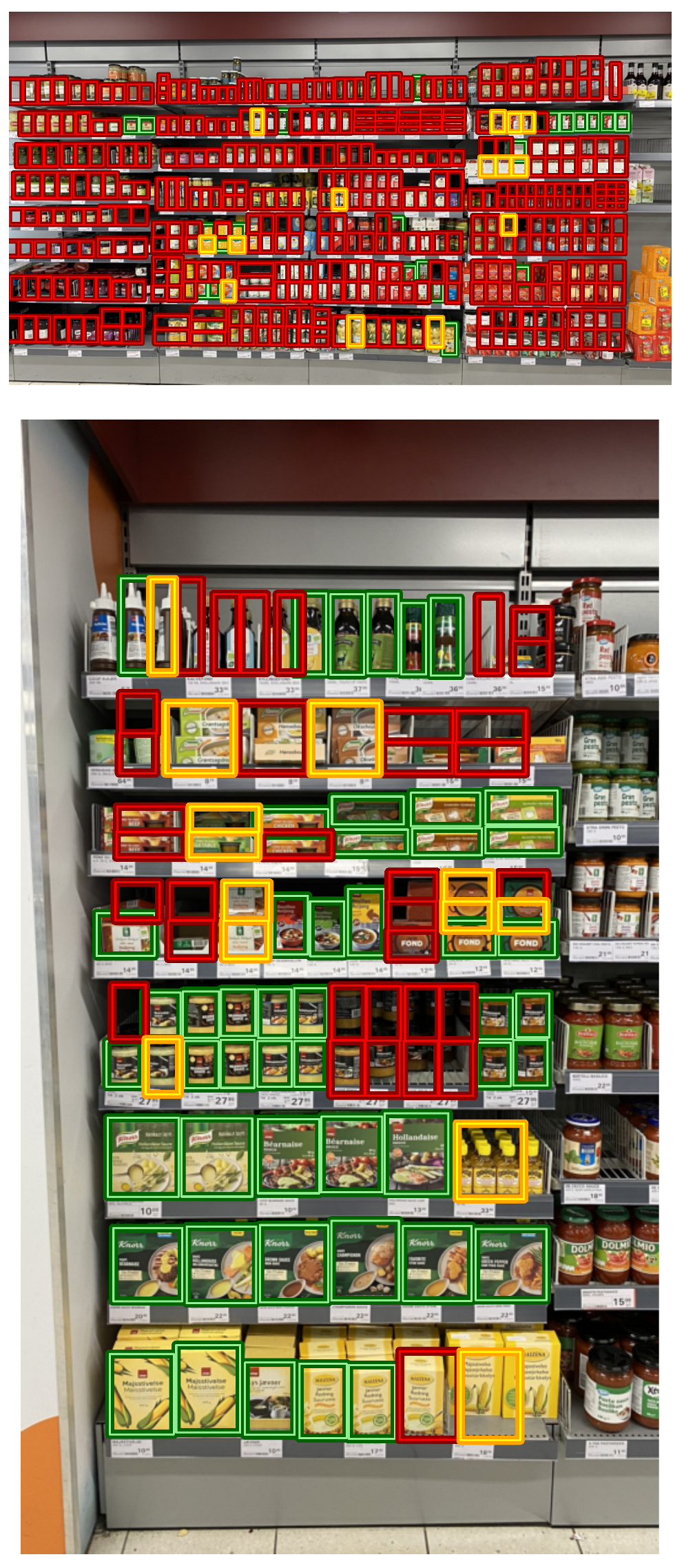
. However, this is mostly due to the classifier performance not being up to par. Figure 12 visualizes the planogram compliance evaluation performance for both the worst- and the best-performing images of our internal dataset using our best model (see Table 5 and

Table 6. Planogram compliance evaluation statistics for each image in the internal dataset, using the model with the lowest $E_{PC}$ (see Table 5). The “Ground truth” and “Detected” values are planogram compliances.

Image	Ground Truth	Detected	$\mathbf{PE}$	${\mathbf{PE}}^2$	${\mathbf{PE}}^2$ std
1	0.697	0.082	−0.616	0.379	0.018
2	0.812	0.612	−0.201	0.043	0.026
3	0.702	0.296	−0.405	0.165	0.017
4	0.569	0.277	−0.292	0.086	0.009
5	0.733	0.279	−0.454	0.207	0.018

). It is evident that even with the worst performing image (Image 1, the top image in the figure) the RANSAC reprojection of the planogram matches the locations of most of the products, yet the classifier does not recognize the products correctly.

Overall, the results show that our approach is a promising option for tackling the difficult automated planogram compliance evaluation problem. However, some further research into the classifier’s accuracy is needed in order to achieve an operationally acceptable level of performance.

4. Conclusions

In this paper, we presented a novel retail product detection pipeline combining a Gaussian layer network product proposal generator and domain invariant hierarchical embedding (DIHE) for classification and utilized it with RANSAC pose estimation for planogram compliance evaluation. We evaluated the performance of our method with two datasets, with the only open-source dataset with planogram evaluation data, GP-180, and our own dataset collected from a large Nordic retailer. We performed the evaluation with a novel metric for evaluating planogram compliance evaluator performance in real-world setups, $E_{PC}$.

The only public dataset for planogram compliance evaluation that we know of is GP-180. This dataset is problematic in several ways: the planograms in GP-180 consist only of information on the position of products relevant to each other instead of in reference to the shelf, all images are fully planogram compliant, and it encompasses only small fractions of whole shelves. This makes the planograms unrealistic. Therefore, we collected our own dataset with the help of a large retailer. The dataset consists of five test pictures encompassing whole racks, corresponding planograms, and iconic images of 7290 products with up to 6 facings each, resulting in 27,204 images in total.

The results showed that our method provided an improved planogram compliance evaluation pipeline, which resulted in accurate estimation solutions when using real-life images that included entire shelves, unlike previous research that has only used images with few products. However, the classification method requires further research to achieve comparable performance using real data as the previous research. Our analysis also demonstrated that our method requires less processing time than the state of the art.

Our approach paves the way for further research that can, eventually, enable utilizing computer vision for the daily in-store planogram operations, thus increasing retail efficiency. The limiting factor of our approach—the product classifier—could be further improved via more sophisticated representation learning methods or by improving the domain adaptation capabilities via substituting the GAN with a latent diffusion model [39], as the latter approach has proven to be superior to GANs in tasks such as image generation and style transfer.