Abstract
Efficiently cutting smaller two-dimensional parts from a larger surface area is a recurring challenge in many manufacturing environments. This point falls under the cut-and-pack (C&P) problems. This study specifically focused on a specialization of the cut path determination (CPD) known as the laser cutting path planning (LCPP) problem. The LCPP aims to determine a sequence of cutting and sliding movements for the head that minimizes the parts’ separation time. It is important to note that both cutting and glide speeds (moving the head without cutting) can vary depending on the equipment, despite their importance in real-world scenarios. This study investigates an adaptive biased random-key genetic algorithm (ABRKGA) and a heuristic to create improved individuals applied to LCPP. Our focus is on dealing with more meaningful instances that resemble real-world requirements. The experiments in this article used parameter values for typical laser cutting machines to assess the feasibility of the proposed methods compared to an existing strategy. The results demonstrate that solutions based on metaheuristics are competitive and that the inclusion of heuristics in the creation of the initial population benefits the execution of the evolutionary strategy in the treatment of practical problems, achieving better performance in terms of the quality of solutions and computational time.
1. Introduction
Researchers frequently aspire to reduce production costs by considering the context of cutting materials. Integrating CAD (computer-aided design) and CAM (computer-aided manufacturing) systems has significantly enhanced the production capacity of device tools for generating NC (numerical control) programs. Consequently, developers have created numerous commercial computer system packages to automate the NC programming process for diverse cutting applications. This advancement has resulted in the extensive adoption of automated devices across manufacturing industries, enabling the precise cutting of various materials such as clothes, papers, glasses, and sheet metals.
For example, cutting clothes involves working with polygon-shaped pieces that must be carefully positioned on a “strip” to minimize waste. This process, known as cutting and packing (C&P), is classified as an optimization problem. It aims to efficiently arrange items within a given space, maintaining the same dimension [1,2]. Employing heuristics and exact techniques for C&P can provide a significant commercial advantage [3]. For comprehensive surveys on C&P problems, refer to [4,5].
In the nesting process, which is the initial stage, the objective is to minimize the amount of raw material required. This process can also involve additional constraints specific to the application at hand. Laser cutting, for instance, is a widely used technique for separating sheet metal items, making it one of the primary methods employed once an optimal layout has been determined.
Once a suitable arrangement of polygons (layout) has been found, the next step is to compute the optimal cutting path the cutting device should follow to minimize the processing time. This problem is known as the cutting path determination problem (CPDP) [6]. The CPDP focuses on determining the most efficient cutting path for a tool or machine to manufacture a specific part or product.
Cutting can be categorized into two main categories: complete cutting, where each polygon is cut entirely before moving on to the next polygon, and partial cutting, where an item can be cut in portions, allowing for switching between partially cut pieces during the cutting process. The CPDP plays a crucial role in the manufacturing industry, and extensive research has been conducted to develop efficient algorithms and approaches to solve this problem across various manufacturing processes. The aim is to optimize the cutting path and minimize processing time, leading to improved efficiency and productivity in the manufacturing industry.
Various studies have explored the impact of laser cutting materials, specifically by examining the effects of processing heat and different speed parameters on cutting quality. However, our research specifically focuses on reducing the empty laser cutting path, mainly when dealing with instances involving connected and separate nested pieces. We incorporate two parameters to represent the air movement () and cutting speeds () of a laser cutting machine. Thus, we are able to simulate the elapsed time to cut the pieces in different paths. It is worth reinforcing that such processes can be time consuming in most applications and gains, however tiny, represent a large improvement overall.
We encounter the laser cutting path planning (LCPP) problem in this context. LCPP is a specific type of CPDP that aims to quickly determine a cutting path that minimizes the overall time required to cut all parts from the given layout. This optimization considers two crucial parameters: and . The total time involved in the laser cutting operation consists of the actual processing time and the movement time, during which the laser head moves without cutting between different nodes and edges (representing the items). Consequently, the actual processing time can be determined once the machine and material cut speed limitations are correctly defined. By optimizing the laser head’s traversal distance between different items, the time spent on air movement can be reduced.
LCPP is an extension of the well-known traveling salesman problem (TSP), a typical NP-hard problem [7]. Consequently, algorithms that aim to provide optimal solutions for LCPP face exponentially increasing computational time as the number of layout pieces grows. Hence, heuristic methods that offer approximate solutions are justified and necessary for solving industrial-scale problems. Metaheuristic methods have gained popularity among researchers as they can discover approximate solutions often close to optimal. On the other hand, approaches based on mathematical formulations have proven impractical for real-world examples, but they can serve as valuable guides for potential methods. This paper presents the self-adapted parameters biased random-key genetic algorithm (ABRKGA) [8] to address the laser cutting path planning problem. We also present a heuristic approach based on Eulerian paths to generate high-quality initial individuals. Our methods outperform existing approaches, and our promising results are compared with those presented in [9] and discussed in detail in Section 4.3.
The rest of this paper is organized as follows: Section 2 provides a formal definition of LCPP, Section 3 presents an overview of current approaches for tool path generation, and Section 4 highlights the critical aspects of the ABRKGA approach and the Eulerian concept for constructing an excellent initial population. Section 5 focuses on the test instances and compares the performance with the best-known solutions, presented in [9]. Finally, Section 6 draws conclusions based on the findings of this research.
2. The Laser Cutting Path Problem (LCPP)
A laser cutting machine is an automated device for precise cutting and design projects in various industries. It offers high cutting speed, narrow kerf, excellent cutting quality, and versatility. The laser cutting path is crucial in determining the cutting quality, processing efficiency, and energy consumption, directly impacting production costs. The required time is divided into cutting and air time (head movement between different edges/patterns) in the laser cutting process. Therefore, the specific CPDP applied to laser cutting machines is known as laser cutting path planning (LCPP).
The primary objective of the LCPP problem is to optimize the cutting time, which depends on two key parameters that simulate the laser cutting device: cutting velocity () and air-moving (or sliding) velocity () of the cutting head. The first parameter is influenced by the machine’s hardware, the shape of the pieces in the input layout, and the characteristics of the material being cut. The second parameter controls the speed at which the cutting head moves without cutting. In this study, we aim to address a generalized type of CPDP [6] considering the earlier constraints, distinguishing it from the research conducted by Derwil et al. [10].
Furthermore, LCPP involves optimizing the distances between cutting points where no cutting is performed, reducing air time. Therefore, strategies must minimize the length of unnecessary laser head movements. This situation can also be considered an “empty trip” problem in laser cutting [11].
Figure 1 illustrates an optimal solution obtained by input layout instance. Note that, in the LCPP problem, the choice process for every solution considers the source (S) coordinates . Usually, the top-left corner of the laser cut machines. The main question is: starting from the source point, how can a laser cutting machine (a computational method) select the best sequence of edges that minimizes the complete cutting process time?
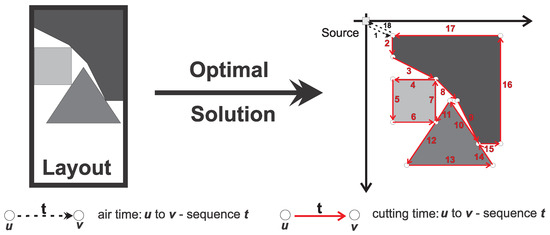
Figure 1.
An optimal solution example for laser cutting path planning.
Furthermore, in Figure 1, the LCPP considers the initial and the final air time (represented by a dashed line, a sequence with the numbers 1 and 18). In every cutting process, the head of the device will move without cutting from the origin to the first point of the input layout (sequence number 1). The same happens when all the edges are cut, and the head must return to the origin (sequence number 18). Thus, it only moves the head when it does not perform a cut. The cost function uses a parameter and the Chebyschev distance between points to compute the time required for that movement. All the rest of the head machine moves (sequences 2–17) increase the final process time to cut the demand of an input layout. For this case, each cut uses the parameter and the size of the edge. Note that the sequence numbers 11 and 12 represent the same edge. Nonetheless, we divide common points for our proposal to increase path possibilities. For example, the node of the square that touches the triangle allows one edge division between sequence numbers 11 and 12.
2.1. Formal Definition
In this paper, we use a graph representation to tackle the LCPP. A graph is an ordered pair of two sets, V the set of vertices and , the set of edges. If , we say that the graph is directed and, if for each element of E we have a value associated with it, we say that the graph is weighted and that is the weight of the edge .
Given a graph , we say that v is adjacent to u if and for a vertex , we call the neighborhood of v in G the set of all vertices adjacent to v in G and denote such a set by . A walk in G is a sequence of edges from G such that, for all we have that and , in other words, the second endpoint of an edge is the first of the next edge. We are given a complete weighted graph with weights for each edge, a set of q required edges such that and two numerical constants, and , representing the cutting speed and the gliding speed for a cutting laser machine.
In this context, the laser cutting path problem (LCPP) can be defined as the optimization problem where one wants to minimize the sum of the weights of the edges in the walk multiplied by the proper speed, meaning that the edges in R must be multiplied by exactly once. All the other edges (including the other appearances of the edges in R) must be multiplied by . More formally, let be a walk in G and be the set of edges obtained from W by removing the first, and only the first, occurrence of an edge in R. We define the cost of W as ; the LCPP problem could be defined as presented in (1).
2.2. An Integer Programming Formulation
A mathematical model serves several purposes. Firstly, it provides a common language that enables effective communication between researchers, practitioners, and stakeholders. Mathematical notation can precisely describe the problem and its requirements, facilitating a shared understanding among different parties.
The model is crucial for formalizing an LCPP: We have two sets of binary variables. The first set of variables are variables that represent wherever the cutting edge is the i-th edge to be cut or not. These variables represent the LCPP solution since this represents the order in which one must cut the pieces. As we know the cut order for the cutting edges, to compute the total cost of this solution, one only needs to determine the edges used as slight edges. Such information is encoded by the second set of binary variables used to represent whether or not we require edge to be used as a sliding edge in the time i. This variable is defined as for all and . Under such variables, we can define the following model.
The objective function (2a) computes the cost of a given solution under the form of an ordering of the required edges; constraints (2b) and constraints (2c) enforce a total ordering of the edges in R, (2c) enforces that each position is an edge, and (2b) ensures that every edge is listed; constraints (2d) compute the movements outside the required edges; and finally, constraints (2e) and constraints (2f) define the bounds on the variables.
Notice that the model encodes the solution as a sequence of edges to be crossed as it is building the path of the solution. Moreover, notice that the formulation has a large number of variables, , and a large number of constraints . The computational results show that this large number of variables take their tool in the formulation and serve as a motivation for the proposition of heuristic methods.
3. Literature Review
Researchers have attempted to apply metaheuristics to various processing methods to minimize the inefficient “airtime” during the operation of cutting devices [12]. GA (genetic algorithm) and BRKGA (biased random-key genetic algorithm) have been used to determine the optimal arrangement of edges for a set of operations located in asymmetrical positions and diverse classes [9,13]. The ant colony optimization (ACO) algorithm has been employed to minimize tool switching time and tool airtime in hole-making operations [14], as well as to discover the optimal travel path by determining the best ordering for hole-cutting operations [15].
The literature encompasses various research studies on algorithmic techniques for CPD. Dewil et al. [7] presented and classified these methods based on the approach used to traverse the vertices of the polygons. They identified three categories: the touring polygons problem [16,17], traveling salesman problem (TSP) [18,19], generalized TSP (GTPS) [20,21], and TSP with neighborhoods (TSP-N) [22].
Derwil et al. [10] classified CPD problems based on the flexibility of selecting an initial contour entry point and whether a piece is partially cut before the cutting head device moves to another object. The first category includes situations with continuous cutting, where the cut can start from any point along the perimeter of the pieces [22,23]. In such cases, the entry point should be the same for both entry and exit. The second category is referred to as endpoint cutting, which pertains to problems where the cut starts and ends at predefined vertices of the polygons [24,25]. The final category is intermittent cutting, which imposes no constraints on the points that can be used to enter or exit the cutting [26,27].
Additional objectives in CPD include minimizing the path length of the cutting trajectory across contours and considering the impact of heat on the cutting path sequence [28]. Another potential constraint is the requirement for a predefined cutting sequence of items without any sliding movements [29]. Manber and Israni [24] addressed the sequencing problem of a torch (flame cutter machine) for cutting regular and irregular parts placed on a surface. Their approach aimed to improve the cutting process by minimizing the number of piercings, which refers to small holes made near each piece.
One approach for solving CPD problems is to use linear integer models to determine the optimal sequence of actions that minimizes the overall cutting time for a given set of parts [30]. Building on this, Dewil et al. [10] further extended the work presented in [30] by incorporating additional constraints that reflect real-world conditions. For instance, the relationships between inner and outer contours arise from holes in parts, pieces positioned within holes, or elements nested within enclosed waste areas. Considering the inner–outer contour relationship means an inner contour must be cut entirely before the outer shape is cut.
In summary, the cutting sequence requires all pieces of an inner contour to be cut before the final element of its outer contour is cut. Additionally, imposing a set of constraints on primary cuts is feasible. In specific layouts, each regular cut is enclosed by a contour formed by its two surrounding contours. Therefore, it is not permitted for a regular cut to connect both of its surrounding contours.
Another set of significant constraints arises from the observation that when a regular cut intersects the contour of two surrounding contours, the disconnected contour can slide, rendering the remaining cutting process infeasible. The laser must move into the cut kerf to achieve precise cutting of the remaining contour objects. This event is not permissible if high part quality is required, and a pre-cut should have been made earlier. Similarly, when cutting a part, a small pre-cut can be created in a neighboring element if the laser head needs to start cutting from that location later on. Dewil et al. [7] also consider several non-trivial extensions, such as collisions, bridges, and thermal effects, which further add to the practical complexities of the problem.
An alternative approach involves mapping CPD to graph-based problems, such as the capacitated node routing problem (NRP), also known as the vehicle routing or dispatch problem [31]. This mapping allows for using mathematical models to optimize CPD [6,32]. These techniques handle CPD by manipulating a mathematical formulation based on the NRP problem and a derived model for the traveling salesman problem (TSP). This strategy is particularly effective in obtaining optimal solutions for instances with approximately 2000 edges within a reasonable time frame. The formulation presented in [6] achieved optimal results for more significant instances, with up to 712 edges and a maximum of 560 nodes.
It is important to note that using mathematical models in practical instances with tens of thousands of edges and nodes has proven impractical. A viable approach is to employ heuristics and metaheuristics to solve graph-based problems equivalent to the original CPD problem. For instance, Moreira et al. [25] adopted this technique by considering the surface as having an elevation (height) and allowing objects to fall as they are being cut. This approach qualifies for exploring alternative strategies that efficiently handle more extensive and complex instances.
Similarly, the empty path problems in laser cutting can be seen as an extension of the traveling salesman problem (TSP), a well-known NP-hard problem. Hajad et al. [33] propose an approach for addressing the laser cutting path problem, formulated as a generalized traveling salesman problem (GTSP). Their study combines population-based simulated annealing (SA) with adaptive large neighborhood search (ALNS). Recombination techniques, such as swap, reversion, insertion, and removal–insertion, are applied alternately using a fitness proportionate sampling mechanism. In each iteration, the cultural algorithm selection method manages 35% of the population to reduce computational execution time while maintaining solution quality. The results indicate that this method can solve problems of various sizes with a reasonable error percentage compared to the best-known solutions.
The study by Hajad et al. [33] demonstrates a promising approach for tackling the laser cutting path problem, utilizing a combination of population-based simulated annealing and adaptive extensive neighborhood search techniques. Their method effectively solves problems of different scales and provides satisfactory accuracy compared to the best-known solutions.
Skinderowicza [34] introduced a modified version of the ant colony optimization (ACO) algorithm called focused ACO (FACO). This approach incorporates a mechanism to manage potential differences between newly generated and previously selected solutions. The main objective is to create a more focused search procedure that allows for the discovery of improvements while maintaining the quality of the existing solution. A computational study using various traveling salesman problem (TSP) datasets was conducted to evaluate the performance of FACO. The results showed that FACO outperforms state-of-the-art ACO algorithms significantly when solving large TSP instances. FACO could find high-quality solutions within less than an hour using an eight-core commodity CPU.
Overall, Skinderowicza’s FACO algorithm presents a promising enhancement to the traditional ACO approach, demonstrating improved performance in solving large-scale TSP instances. The efficient computational performance of FACO makes it a valuable tool for tackling optimization problems with practical significance.
It is worth noting that mathematical formulations have proven to be impractical for more real-world examples. A practicable technique is using metaheuristics that employ a graph-based representation similar to the traditional CPD problem. However, we incorporate the air and cut speeds as additional considerations. We employ the adaptive biased random-key genetic algorithm (ABRKGA) [8], combined with an Eulerian heuristic, to construct the initial population and generate new individuals during the entire execution process.
By integrating the ABRKGA and the Eulerian heuristic, we aim to overcome the challenges posed by practical instances and enhance the efficiency of the solution process. This hybrid approach combines the benefits of both metaheuristics and heuristic techniques, allowing us to explore the solution space effectively and generate high-quality initial solutions.
In general, the proposed approach of utilizing the ABRKGA and Eulerian heuristic in conjunction with a graph-based representation addresses the limitations of traditional mathematical formulations. This combination of techniques provides a promising framework for solving practical CPD problems, considering the complexities of real-world scenarios and optimizing the air and cut speeds.
4. Overview of Application of ABRKGA to LCPP
4.1. Introduction
Metaheuristics serve as practical tools for acquiring high-quality solutions to combinatorial optimization problems. Nevertheless, during the design phase, developers must carefully consider various aspects, including solution representation, objective function calculation, constraints handling, neighborhood structures, initial solution selection, and parameter configuration. These decisions present numerous alternatives, and selecting the most suitable options becomes essential in attaining reasonable solutions for a given optimization problem.
The biased random-key genetic algorithm (BRKGA), put forward by Goncalves and Resende [35], presents an evolutionary algorithm that streamlines several choices mentioned above. It relies on the notion of random keys to depict a solution and employs a decoder function to transform the random-key solution into an optimized solution for the problem. Consequently, developers must implement the problem-specific decoder and adjust the method’s parameters.
Nonetheless, a crucial aspect of metaheuristics is the impact of parameters on the efficiency and effectiveness of exploring the solution space. These parameters necessitate configuration in every metaheuristic. However, the values are only sometimes optimal for specific problems or instances, and they may not be suitable considering the available computational time for execution. Consequently, conducting an efficient configuration of parameter values utilized in each specific application is essential.
The execution of evolutionary algorithms can involve configuration parameters as constants at the beginning of the execution or allowing flexibility in adjusting them as the process unfolds. In [36], the authors present a classification of parameter configuration techniques for evolutionary algorithms. Parameter values can be predetermined before the execution and remain fixed throughout the search (offline), or the parameter values can be dynamically modified during the execution (online).
In this section, we present a self-adapted params BRKGA, [8] (ABRKGA), aiming to balance exploration and exploitation considering the context of LCPP representation. The parameter values are modified according to deterministic rules (e.g., varying over the number of iterations) or adapted based on information obtained during the search (e.g., the quality of the solution found). Parameters can also be included in the solution representation and evolve during the search process (self-adaptive control). We know this approach does not necessarily reduce the number of parameters; however, the authors proposed simplifying the parameter configuration. Figure 2 depicts the evolutionary progression of the proposed ABRKGA.
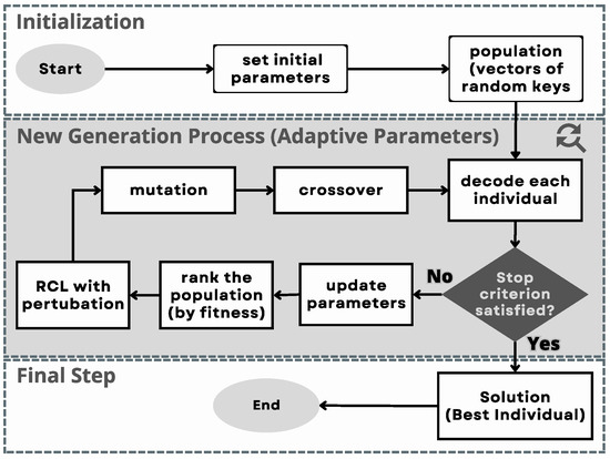
Figure 2.
The ABRKGA workflow. Adapted from [8].
4.2. Initialization and Basic Concepts
Similarly to [9], the execution will be performed on a laser cutting machine that moves along coordinates (x, y). The input parameters will define the head movement speed () and cutting speed (). These values may vary according to equipment needs. The Chebyshev distance was considered to calculate the required time for a machine to extract parts from the inputs.
The input parameters of our approach include the following:
- p—population size (representing the set of solutions viable in each iteration);
- —elite size partition of the population (representing the portion of the population that is selected as elite);
- —mutant size partition of the population (representing the portion of the solutions that are submitted to our mutation procedure);
- —probability of inheriting the key from an elite parent;
- —maximum number of generations;
- —value based on the running available time and ();
- —the device head movement speed value;
- —the device head cutting speed value.
We apply five classical parameters of BRKGA [37] (), and also consider (, , ) (ABRKGA) [36] and (,), specific parameters of LCPP. The variables and exhibit self-adjusting characteristics, while the remaining variables are modified using deterministic principles, except and which are constant for the whole execution. Users must specify a solitary fresh parameter depending on the available duration of execution. The objective of the ABRKGA is to employ parameter adjustment to facilitate increased exploration during the initial stage of the search and enhanced exploitation throughout the evolutionary progression.
The ABRKGA creates an initial population comprising p randomly generated key vectors (individuals). Each individual’s chromosome consists of genes, randomly generated with a uniform probability from the range [0, 1]. The representation of a possible solution for LCPP is divided into three parts. Each individual is encoded by a vector of random keys (1, 2, …, n, n + 1, …, 2n, 2n + 1, 2n + 2), where n corresponds to the number of edges () that must be cut from the input layout. The n’s first positions define the cutting order of each required edge, and the next n’s indexes denote the direction of the cut. Finally, the remaining positions () and () are utilized to calculate the self-adjusting parameters and , correspondingly. Figure 3 illustrates the three elements of individual representation.
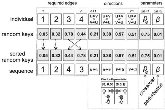
Figure 3.
Encoder and decoder for an individual representation.
It is necessary to emphasize that the cutting process starts from the original system of each device (source) and returns with the movement head at the end (regress). This research considers point (0,0) as the source because the industrial cutting machine applies the same idea. In this context, Figure 4 shows a visual solution considering an input layout and the same individual presented in Figure 3.
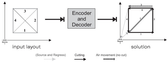
Figure 4.
Input layout and solution constructed, for example illustrated in Figure 3.
Therefore, the fitness of each individual () and, consequently, the quality of the solutions is linked to the cutting time of an input layout. It is crucial to compute the fitness function for each i to count the time to cut the necessary edges () and the movements of the head from the origin to the initially chosen node of the layout and back to the source (). Then, we use the head movement speed () and cutting speed () to calculate the value of .
Figure 5 shows the (i, i + 1) step of the function. Note that (i) typifies the edge to be cut in time(i), and () the direction, see Figure 3. The position and indicates that the edge labeled with 4 must be separated with the direction of nodes (). Note that the complete cutting time () is incremented by . The next element, and , needs to perform the air movement only to then cut edge 5 in the direction (). Thus, add to . The time considered to cut in i and is computed by this function :
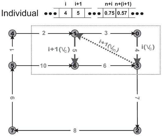
Figure 5.
Example of the quality value computed between i and indexes of individual vector representation.
In other words, the faster the cut is made, the higher the quality of the individual. Therefore, Equation (4) denotes the fitness function for an individual i, Equation (5) denotes the best individual i of a population P, and Equation (6) the quality of a population k. These concepts are expressed more formally as:
The quality of the solutions generated and inserted into the population, either initially or during the execution of the evolutionary algorithm, has a positive impact when associated with some knowledge about the problem at hand. In light of this, we apply a strategy to transform the input graph (computational representation of the layout) into another graph containing at least one Eulerian path. Thus, this heuristic guides the construction of the initial population. Section 4.3 describes the heuristic in the context of solutions for the LCPP.
4.3. An Eulerian Heuristic to Generate Improved Individuals for LCPP
Consider an LCPP context. Examine the provided layout (Figure 6) and note that it can commence from a single point and traverse every edge precisely once without changing the device mode (always cutting). The term traversable describes graphs in which it is possible to begin at a vertex and trace all the edges without lifting the pen off the page or retracing any edge. There are two categories of traversable graphs:
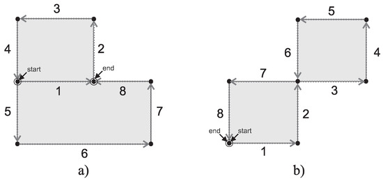
Figure 6.
Each graph has a trail that utilizes each edge exactly once. The trail on the left (a) is open, commencing and ending at different vertices. Conversely, the graph on the right (b) is closed, allowing any vertices to be the start and end points.
- A graph is called Eulerian if it possesses a closed trail, known as an Eulerian trail or an Eulerian circuit, which starts and ends at the same vertex while traversing every edge.
- A graph with an open trail, where the trail begins and ends at distinct vertices while traversing every edge, is called semi-Eulerian. Alternatively, it can be denoted as having a semi-Eulerian trail.
It is feasible to ascertain whether an undirected graph is Eulerian or semi-Eulerian without the need to identify the trail explicitly: if a graph exhibits precisely two vertices with an odd degree, it is classified as semi-Eulerian (Figure 6a). These two vertices serve as the start and end points of the open semi-Eulerian trail. If a graph consists entirely of even-degree vertices, it is categorized as Eulerian (Figure 6b). The closed Eulerian trail can commence from any vertex within the graph.
In this context, we consider the concept, as mentioned earlier, to improve individual fitness, whereas solutions tend to have fewer unnecessary air moves. In [9], the authors construct the initial population with a random order of edges. This fact impacts several air movements. Our idea is to consider four specific cases on the generation of initial solutions:
- We assume the input layout is connected and contains all nodes with even degrees (Eulerian graph). Then, the heuristic can find an Eulerian circuit and needs to use one air movement (source to nearest node) and another (nearest node back to origin). In this case, we have the minimum time required to cut all items.Note: To return the sequence of edges at the Eulerian circuit, we apply a linear time implementation adapted from [38] with NetworkX (Python library).
- We assume the input layout is connected and contains precisely two vertices that have odd degrees (semi-Eulerian graph). In this way, the initial population comprises solutions with path routes that necessarily pass through both odd-degree vertices. The idea is that the metaheuristic finds the combination that minimizes the end-cut time in the LCPP, assuming that a good solution must pass through the starting and ending points.
- We assume the input layout is connected and contains more than two nodes with odd degrees. In this case, the heuristic seeks to transform the graph’s vertices that have odd degrees into even degrees, adding new edges between them until only two odd edges remain in the semi-Eulerian graph (2).
- We consider the possibility that the input layouts present items without contact between them. This situation occurs when the cut needs to maintain a safe area for the edges.
In this procedure, edges between odd vertices enter the solution and are counted as displacement. Algorithm 1 shows the pseudocode for applying the heuristic to the graph. First, the edges are divided into two sets with even and odd degrees, then the code checks if the graph is semi-Eulerian. Otherwise, the displacements are added between them until only two even vertices remain.
Algorithm 2 shows the pseudocode of how we apply the heuristic to individual generation. Initially, we select a vertex and edge of this vertex, add it to the individual, and later, walk on the edges that can be reached from the initial vertex. When it is not possible, we choose another vertex that was not selected, repeating the process until all edges of the graph are covered.
| Algorithm 1: Eulerian Heuristc Algorithm |
 |
| Algorithm 2: Eulerian Heuristic Individual Generation |
 |
4.4. New Generation Process
During the core stage of the algorithm, the ABRKGA metaheuristic comprises six components in every successive iteration. The first step is to decode each individual, described in Section 4.2. The upper limit of generations determines the termination condition for ABRKGA, computed using the parameter . The population size in each generation is adjusted using the same parameter. Note that the value of is determined in the initialization phase, considering the allotted run time.
The parameters undergo updates based on deterministic rules that consider the advancement of the evolutionary process. The evolutionary process defines the two self-adaptive parameters and as they are included within the chromosomes; see Figure 3. We explain the methodology of online parameter control during the search process, aiming to enhance population variance and prevent premature convergence, considering population size, number of generations, top/mutation partitions, and the crossover process.
Defining the parameter p is complex for real-instance problems. Furthermore, varying sizes could be advantageous during different stages of the search. For instance, at the beginning of the process, a larger population size may be beneficial to explore the search space and discover promising regions. As the subsequent generations progress, reducing the population size could be advantageous for refining the solutions.
According to [39], users of BRKGA typically select a population size ranging from 100 to 1000 individuals. It is worth noting that choosing smaller populations may lead to premature convergence towards local minima due to the limited information in the elite partition. Conversely, employing substantial populations increases computational time.
In this context, the new generation process initiates with the maximum population size (p = ). As each generation progresses, the population size (p) for each generation (k) diminishes by a factor of:
The quantity of offspring is adjusted to determine the size of the new population, which is defined by Equation (7). This strategy reduces the possible solutions at each generation. Then, a restart procedure is executed when the population size falls below a threshold of individuals. This restart procedure involves preserving only the restricted chromosome list (RCL) individuals, explained next, in the current population while generating new individuals at random.
Additionally, these parameters are utilized in the calculation of the stop criterion through Equation (8), which determines the maximum number of generations () for the ABRKGA. Consequently, a minor reduction in population size (with values close to 1) results in fewer generations. Conversely, if the population size decreases faster, it necessitates more generations and restarts.
In order to generalize, the population chromosomes are arranged in ascending order, placing the best chromosomes at the top and the worst at the bottom. This arrangement applies to minimization problems, as is the case for LCPP. The population is divided into two groups, with the best individuals retained in a restricted chromosome list (RCL). The RCL consists of individuals whose fitness surpasses a threshold value () determined by the parameter within the range [0, 1]:
The fitness of the best individual in the current population is denoted as , while the fitness of the poorest individual is represented as . When = 0, only individuals with the highest fitness are included in the RCL, whereas = 1 includes all individuals in the RCL. The value of parameter is adjusted periodically based on the progress of the search. The maximum number of individuals that can be included in the RCL is limited by . Lastly, the individuals in the RCL are replicated and carried over to the next population.
The parameter determines the number of elite individuals by influencing the size of the RCL (defined by Equation (9)). Initially, is set to and decreases with each generation according to Equation (10). The minimum value for is . This range accounts for the suboptimal solutions commonly encountered in the early generations and the tendency for population stagnation after a certain number of iterations. This range was considered equality in the proposal of Chaves et al. [8].
The parameters (ranging from 0.10 to 0.25) and (ranging from 0.05 to 0.20) are employed to determine the elite () and mutant () partitions within the population. Once again, the objective of the search process is to promote diversification during the initial phase and gradually intensify the focus as the population evolves.
The parameter control is defined by Equation (11), while is defined by Equation (12), with representing the current generation. Consequently, the maximum size of the elite partition is smaller in the early generations when the average quality of individuals is lower. However, this number progressively increases in subsequent generations. Conversely, the number of mutants decreases as the search process unfolds.
In order to maintain diversification within the RCL, perturbations are employed to enable the ABRKGA to break free from local optima and overcome the limitations of solely introducing random individuals. Identical fitness values solely determine the similarity between individuals, for simplicity. This perturbation strategy involves randomly swapping values in a vector of random keys, with the strength of perturbation defined by the self-adaptive parameter , which ranges from to .
A random variable is generated for each chromosome gene for each similar individual. This random variable determines whether a specific random key will undergo modification through gene swaps at random positions. This probability is set to a low value, otherwise, the search process may devolve into randomness. The parameter is included in position of the chromosome and evolves alongside the other genes associated with the problem.
Within this framework, individuals with identical fitness values are subjected to perturbations, with the intensity of perturbation determined by , a self-adaptive parameter. The value of , calculated using Equation (13), is incorporated into chromosome c at position and undergoes evolutionary changes.
The mutation stage produces a set of mutant individuals through a random generation process. The identical module for generating the initial population creates these mutants.
The crossover process combines pairs of parents through mating, with one parent chosen from the RCL and the other randomly selected from the remaining population. The parameterized uniform crossover technique [40] is applied, which involves generating uniform random numbers within the range of for each gene of the chromosome. For each gene position j, if is less than or equal to , then the offspring inherits the j-th allele from the RCL parent; otherwise, it inherits the allele from the other parent. The value of the self-adaptive parameter , located at position of the chromosome, is always selected from the non-RCL parent.
The parameterized uniform crossover is designed to prioritize the inheritance of alleles from the RCL parent chromosomes. This method is achieved through the self-adaptive parameter , which determines the probability of an offspring inheriting the vector component from the RCL parent. The calculation of , as defined by Equation (14), involves the utilization of the random-key from the non-RCL chromosome c.
It is essential to point out that the values for defining the calculations of the ABRKGA control parameters equations are based on the work of [39,41]. Table 1 presents each suggested value range for the parameters applied. Furthermore, the parameter is a configuration parameter, but it is relatively straightforward to adjust. Like in [8], we have defined three specific values for based on the available running time. All of these values lead to a gradual decrease in population size. The primary distinction lies in the maximum number of generations, affecting the running time and solution space. Table 2 provides an overview of the and values and their respective characteristics. p1: The search is conducted within a reasonable computational time, ensuring that the minimum population size remains around 70% of the initial population size. p2: The search process is executed within a reasonable time, necessitating the restart of the population to its maximum size once. p3: The search is carried out over an extended duration, requiring four population restarts to be performed.

Table 1.
Parameter definitions and recommended value ranges.
Table 2.
Available options for parameter .
The objective of the ABRKGA is to utilize parameter tuning to enhance exploration during the initial phase of the search and increase exploitation throughout the evolutionary process. The evolutionary process of the ABRKGA is depicted in Figure 2. The decoder represents the problem-dependent component, responsible for converting random-key vectors into solutions and evaluating their fitness. On the other hand, the remaining components are problem-agnostic and can be reused in a general-purpose framework. Using an Eulerian path heuristic, we also consider a specialized initial population and new individual mutation. Algorithm 3 provides the pseudocode for our adaptation for ABRKGA to tackle LCPP. The procedure’s input parameters are the required cutting edges (n) and the specific ABRKGA parameter .
| Algorithm 3: Pseudocode of ABRKGA to tackle LCPP |
 |
5. Computational Results
The computational experiments were performed on a machine with a max turbo clock speed of 4.90 GHz, 11th Gen Intel(R) Core(TM) i7-11700 processor, 16 GB RAM, and running the Windows 10 operational system. All algorithms were implemented using the Python language version 3.7. The input data consisted of layout instances extracted using the research developed by Amaro et al. [41], resulting in SVG files. The subsequent sections provide details about the benchmark instances (Section 5.1), the results obtained with the execution of the LCPP model (Section 5.2), a comparison between BRKGA x e-BRKGA (Section 5.3), ABRKGA without and with an improved initial population with the Eulerian heuristic (Section 5.4), called here e-ABRKGA, and the e-BRKGA x e-ABRKGA in Section (Section 5.5). Please refer to the Data Availability Statement for complete information on the data used and constructed in this paper.
5.1. Instances
We utilized a set of 50 problem instances to evaluate the presented approaches. These instances were categorized based on the possible presence of space between the pieces in the input layout, categorized as connected (C) instances (see Figure A1 and Figure A2 in Appendix A.1) or separated (S) instances (see Figure A3, Figure A4 and Figure A5 in Appendix A.2). The space between items in the latter group enables the utilization of support, which is common in particular material cutting applications. We generated the dataset using the nesting approach outlined in [41], and for all tests, the laser machine parameters considered, (cut) and (air), were 16.67 mm/s and 400 mm/s, respectively.
In [9], several hyperparameter settings have been tested for the GA and the BRKGA heuristics, executed ten times for each instance. The authors chose the best-performing configuration, which will be compared with our approach. In Table 3, we present the instances along with the corresponding number of vertices, the count of edges (for both the original and adapted layouts with the edge joints), and the number of polygons. We also tested ABRKGA with the value of presented in Table 2 and we have chosen to use a maximum () and minimum (), executing each instance ten times.
Table 3.
The properties of each instance were applied in our computational experiments. The table presents each instance’s number of nodes, edges, and polygons: (C) connected pieces and (S) separated.
Some instances present different vertices and edges due to applying the join procedure and split edges in the original input layout. It is necessary to highlight that joining segments are treated as particular cases of splitting edges. The algorithm of preprocessing input data, extracted by [6], converts the input file into a graph before addressing the LCPP. This conversion process can increase the number of edges of the original layout due to the realization of edge separation that occurs when a node of one figure touches the edge of another. For example, in Figure 6a) the “end” point separates edge 1 and edge 8. This procedure needs to occur to connect (C) groups of instances.
5.2. Results for the MIP Flow Model
In this subsection, we report the results obtained for the proposed MIP model. The model was implemented in JULIA 1.8.1 using JuMP library version 0.9, and the computational tests were carried out on a machine with a Linux Ubuntu 20.04 operational system, 16 GB of RAM, and an i7 processor with eight cores and 2.7 Hz speed. We set a time limit of 1 h (3600 s) for each instance. This value was adopted arbitrarily to establish a time control for the execution and validation of the model on the tests. The significance of 3600 s was considered reasonable by our team. We aim to consider the optimal results obtained and check with the BRKGA, ABRKGA, and variations.
Table 4 and Table 5 present results for the MIP flow model in the set of instances connected and separated. The column instance notes the name of the instance; column solution reports the best solution obtained by the model; column time is the elapsed time in seconds if the model reached the time limit of 1 h, this is represented by LIMIT; column gap registers the gap as presented by the solver at the end of execution; and column nodes reports the number of nodes in the branch and bound tree.
Table 4.
Results for the MIP flow model on the connected set of instances.
Table 5.
Results for the MIP flow model on the separated set of instances.
We filter instances containing a maximum of 40 nodes to carry out tests with the model. The results of Table 4 and Table 5 show that the MIP model can only solve a small number of the instances (four in both cases), and the instances that were solved have a small size (number of vertices plus the number of edges). One can verify that the models reach the time limit for most instances. Furthermore, for some instances, it was trapped in the root node of the branch and bound tree, and for the instance blaz2 of the separated benchmark, the model could not even be produced due to memory issues.
All these remarks lead us to conclude that, although this model presents a theoretical contribution to LCPP, it still needs to be a practical method, and heuristic methods are needed to tackle large instances. However, we intend to use the results presented by the model as an initial guide for the solutions of the computational experiments proposed in this research.
5.3. Comparison of Results for BRKGA vs. e-BRKGA
This section shows the first comparison between some strategies discussed in the context of this paper. Thus, the results of BRKGA, as presented by [9], are confronted with the same strategy. However, we incorporate the Eulerian heuristic into the mechanism for creating the initial population. We will refer to this approach as e-BRKGA to simplify the terms.
The same parameters () were applied to both approaches, and the stopping rule was approximately 300 s of time execution or 100 generations without improvement on the best solution found. Table 6 (BRKGA) and Table 7 (e-BRKGA) present the best, worst, average, standard deviation, and coefficient of variation for the ten computational runs of each instance from the connected group (C). The same structure was adopted in Table 8 (BRKGA) and Table 9, except that these two other tables represent execution for the separated group (S).
Table 6.
BRKGA applied to the connected set of instances (C).
Table 7.
e-BRKGA applied to the connected set of instances (C).
Table 8.
BRKGA applied to the separated set of instances (S).
Table 9.
e-BRKGA applied to the separated set of instances (S).
The first point deserving highlight in the analysis of the results is the average computational time of the approaches. Considering the “average” column, the average computational time for all executions in Table 6 was 170.70 s. In contrast, in Table 7, it is possible to observe that the e-BRKGA required a time 41.30% less than BRKGA, approximately 100.20 s. Considering the group (S), the average execution times of instances (Table 8) is 183.43 s, while the same attribute found in Table 9 is 96.17 s. This fact characterizes a gain of 47.57% of the e-BRKGA with respect to the BRKGA.
The coefficient of variation (variation column) allows the determination of the precision of the measurements and the variability within samples. Regarding the execution time, we highlight the variation in the instances “blaz1”, “dighe2”, and “inst_9pol” from group (C), which were the only ones that showed values higher than 10% (moderate variation).
In the instances from Table 7, the entries “dighe1”, “inst_2pol”, “inst_4pol”, and “shapes2” also fall under a moderate aspect regarding the variation in the samples. The only instance that draws attention to the context of the coefficient of variation is “inst_6pol”, with a value of 21.79%. Even so, there still needs to be a sizable relative variability in the data about the mean. Table 8 and Table 9 present the execution time variation, presenting all values less than 10%.
In summary, we can consider the execution times based on their respective averages due to the low value of the coefficient of variation attribute. We also highlight that 76% of the instances in group (C) and 80% in group (S) have GAPs (see Table 10) more significant than 50% concerning the difference in execution times for e-BRKGA.
Table 10.
GAP comparison BRKGA x e-BRKGA to connected (C) and separated (S) instances.
Even in the column of the best and worst solutions found, when the developed Eulerian heuristic is applied to the initial population, it presents gains in execution time when applying e-BRKGA to LCPP. In the group of instances (C), only four instances had a longer execution time for e-BRKGA. However, for the set (S), no e-BRKGA execution took more computational time than BRKGA. All evolution graphs (best individual fitness x number of generation) are available in Data Availability Statement.
To consider the quality of the solutions (objective function value), as the second point of analysis of the results, Table 6, Table 7, Table 8, Table 9 and Table 10 reveal the best and average solutions of each approach and the “GAP” column that presents a comparison between the potentials (solution quality and computational time) of each strategy. For the two values incorporated in the “GAP” column, if the “fitness” or “time (%)” values are positive, it indicates a percentage gain. This improvement can be either in terms of the average solution quality or the execution speed of e-BRKGA compared to BRKGA or vice versa, depending on the sign.
For example, consider the “albano” instance, the first row in Table 10. The “fitness (%)” value in the “GAP connected” column between the approaches is 7.68%, and regarding the “time (%)” column, it is −1.66%. These numbers mean that the value of the “fitness” column for the e-BRKGA average multiplied by (1 + 7.68%) is approximately equal to the average “fitness” of the BRKGA. Furthermore, the “time (%)” column value for the “GAP connected” implies that the BRKGA executed in a time that, when multiplied by (1 + 1.66%), is approximately equal to the time spent by e-BRKGA. A positive GAP percentage represents gains to e-BRKGA in the proportion . Otherwise, the improvement is reached by the BRKGA approach.
From Table 10, it is possible to verify that the BRKGA achieved a better average in the quality of results in 17 instances (negative percentages), tied in 2, and lost in 6 when considering the group of instances (C). For this analysis, it is essential to observe that among the six instances where e-BRKGA had a better average fitness, five have the highest number of nodes and edges in the input graph: “albano”, “blaz3”, “inst_26pol”, “shapes4”, and “trousers”; see Table 3.
Notice that e-BRKGA found, on average, a 7.68% improvement, with an execution time 1.66% higher, meaning 5.04 s slower than BRKGA, considering the “albano” instance. A more significant gain occurs with the “inst_26pol” instance, reaching a 10.69% improvement with a 3.34% longer execution time. In “trousers”, the average fitness gain was 6.31% in 28.88 s (−9.28%) more for the algorithm to stop.
On the other hand, in some instances, e-BRKGA improved compared to BRKGA, both in the average fitness and execution time. The entries “blaz3” and “inst_7pol” demonstrated slight gains in fitness, 0.13% and 0.02%, respectively. However, in terms of execution time, the improvement reaches 34.85% (105.50 s) for “blaz3” and 72.35% (45.77 s) for “inst_7pol.
For the group of separated instances (S), the results exhibit similar characteristics of (C), except for the execution time of e-BRKGA, which is better in all instances. In this examination, it is crucial to note that out of the five instances where e-BRKGA showed a superior average fitness: ”albano“, “inst_16pol”, “inst_26pol”, “shapes4”, and “trousers”.
The conclusion of this initial round of test analyses is well supported in Table 10. The strategy of initializing the population with the Eulerian heuristic for LCPP directly influenced the two aspects discussed here: solution quality and computational execution speed. Notably, in both the group (C) and group (S) datasets, the difference in fitness values when BRKGA averages better is relatively small, less than 2%. This information leads to the preference of the e-BRKGA approach over BRKGA for the LCPP problem, considering the computational execution times.
5.4. Comparison of Results for ABRKGA vs. e-ABRKGA
This section presents the second comparison between the ABRKGA strategies within this paper, explicitly pitting them against the same strategy that incorporates the Eulerian heuristic in the mechanism for creating the initial population. Through this comparison, we aimed to evaluate the performance of both ABRKGA variants and the Eulerian heuristic-based procedure.
The set of three parameters for were applied for both approaches. Table A1 (ABRKGA) and Table A2 (e-ABRKGA) show the best, worst, mean, standard deviation, and coefficient of variation for the ten computational runs of each instance of the connected group (C). The same structure was adopted in Table A3 (ABRKGA) and Table A4 (e-ABRKGA), except that these two other tables represent the execution for the separate group (S).
In this second analysis, the first point that deserves attention in analyzing the results is the average time of the approaches. Considering the “average” column, the average time of all executions in Table A1 was 86.09 s. On the other hand, in Table A2, it is possible to observe that the e-ABRKGA required a time 219.69% longer than the ABRKGA, approximately 275.18 s. Considering group (S), the average execution time of the instances (Table A3) is 101.04 s, while the same attribute found in Table A4 is 179.04 s. This is a 77.2% gain for ABRKGA over e-ABRKGA.
In Table A2 and Table A4, the variation in execution times all show values less than 15%. In e-ABRKGA, both the instances of groups (C) and (S) presented a longer execution time because they use their stopping criteria. All evolution graphs (best individual fitness x number of generation) are available in the Data Availability Statement.
To consider the quality of the solutions, as the second point of analysis of the results, Table A1, Table A2, Table A3, Table A4 and Table A5 reveal the best and average solutions of each approach and the “GAP” column that maintains the comparison between the potentials (solution quality and computational time) of each strategy. For the two values incorporated in the “GAP” column, if the “fitness” or “time (%)” values are positive, it indicates a percentage gain. This improvement can be either in terms of the average solution quality or the execution speed of ABRKGA compared to e-ABRKGA or vice versa, depending on the sign.
From Table A5, it is possible to verify that e-ABRKGA obtained the best average in the quality of the results in 48 instances with its set of parameters (positive percentages), tied in 5, and lost in 22 when considering the group of instances (C). For the (S) instances, the e-ABRKGA only lost in the “trousers” instance with .
Notice that e-ABRKGA found, on average, a 6.7% improvement, with an execution time 152.1% higher, meaning 125.05 s slower than ABRKGA, considering the “albano” instance with .
For the group of separate instances (S), the results show similar characteristics to (C), except for the execution time of e-ABRKGA, which is worse in all instances. In this examination, it is essential to note that in almost all instances e-ABRKGA presented a superior average fitness.
The results from the second round of test analyses are strongly supported by the data presented in Table A5. The strategy of initializing the population with the Eulerian heuristic for LCPP had a direct impact, now negative, assuming the relation solution quality versus computational execution speed. Particularly noteworthy is the observation that in the datasets of groups (C) and group (S), the difference in fitness values when the average ABRKGA result is superior is relatively small, being less than 3%. Simultaneously, the ABRKGA approach demonstrated execution times up to 500% shorter than the e-ABRKGA method. These results show that the ABRKGA approach outperforms the e-ABRKGA approach for the LCPP problem, particularly when considering computational execution times. Therefore, for practical applications where efficiency is a significant factor, the ABRKGA strategy is the preferred choice.
5.5. Comparison of Results for e-BRKGA vs. e-ABRKGA
This section shows the third comparison between strategies incorporating the Eulerian heuristic in Section 5.3 and Section 5.4. The e-BRKGA is compared using the parameters ; and the e-ABRKGA with the parameters .
In this third analysis, the first point that deserves attention in analyzing the results is the average time of the approaches. Considering the “average” column, the average time of all executions in Table 7 was 100.20 s. On the other hand, in Table A2, it is possible to observe that the e-ABRKGA required a time 174.63% greater than the e-BRKGA, approximately 275.18 s. Considering group (S), the average execution time of the instances (Table 9) is 96.17 s, while the same attribute found in Table A4 is 179.04 s. This fact characterizes a gain of 86.17% for e-BRKGA with respect to e-ABRKGA.
To consider the quality of the solutions as the second point of analysis of the results, Table 7, Table 9, Table A2, Table A4 and Table A6 reveal the best and average solutions of each approach and the “GAP” column that presents the comparison between the potentials (solution quality and computational time) of each strategy. For the two values incorporated in the “GAP” column, if the “fitness” or “time (%)” values are positive, this indicates a percentage gain. This improvement can be either in terms of the average solution quality or the execution speed of e-BRKGA compared to e-ABRKGA or vice versa, depending on the sign.
From Table A6, it is possible to verify that e-ABRKGA obtained the best average in the quality of the results in 41 instances with its set of parameters (positive percentages), tied in 6, and lost in 28 when considering the group of instances (C). For the (S) instances, the e-ABRKGA lost in 30, tied in 7, and won in 38 instances.
Note that e-ABRKGA found, in the best result, an improvement of 4.65%, with an execution time 847.78% higher, that is, 2882.43 s slower than e-BRKGA, considering instance “albano” with for group (C). For group (S), the result was similar, an improvement of 5.15%, with an execution time 512.91% higher, that is, 1570.11 s slower than e-BRKGA, considering the instance “albano” with .
The findings of this third round of test analyses are strongly substantiated by the data presented in Table A6. Using the Eulerian heuristic in initializing the population for LCPP impacted the two aspects under consideration: solution quality and computational execution speed. It is worth noting that in the group (C) and group (S) datasets, the disparity in fitness values when the average e-BRKGA result is superior is relatively minor, generally below 3%. Moreover, the e-BRKGA approach exhibited significantly shorter computational execution times, often up to 1000% faster.
These results consistently point to the superiority of the e-BRKGA approach over e-ABRKGA when considering the LCPP problem and its computational execution times. The e-BRKGA strategy outperforms the e-ABRKGA variant, striking a commendable balance between solution optimality and computational efficiency. Therefore, for practical applications with faster results, the e-BRKGA approach emerges as the more favorable choice over the e-ABRKGA approach.
6. Conclusions
This research paper presents the LCPP (laser cutting path planning) problem, which effectively captures real-world conditions by evaluating distinct cutting and air-moving speeds. The consequence of cutting and sliding rates in actual machinery is often overlooked in the existing literature, making this investigation a valuable contribution to the field. By presenting a self-adaptive parameters evolutionary approach, namely, the adaptive biased random-key genetic algorithm (ABRKGA), and a heuristic to try to construct more significant fitness of individuals, the authors demonstrate their effectiveness in tackling practical instances of the problem. These methods hold promise in addressing functional challenges related to the LCPP in real-world systems.
Computational tests were conducted to conclude our investigation, comprising four distinct scenarios and considering 50 available instances in the literature [9]. In the first scenario, tests are conducted using the conceptual model in mathematical programming proposed for the LCPP (Section 2.2). Our findings revealed that the optimal solution was obtained only for instances containing a maximum of 20 nodes and 20 edges within a runtime limit of 1 h.
The other three experiments (Section 5.3, Section 5.4 and Section 5.5) were designed to facilitate a comparative analysis between solution quality and execution time. By conducting these experiments, our objective was to assess how different approaches or algorithms perform in terms of finding high-quality solutions within a limited time frame. This comparison allows us to understand the trade-offs between solution optimality and computational efficiency, providing valuable insights into the strengths and weaknesses of each method under consideration. Such an analysis is crucial in selecting the most suitable approach for practical applications, where finding reasonably good solutions is often paramount. In this context, we conclude, through the analysis of the test tables, that applying the heuristic in conjunction with BRKGA provided the best trade-off between solution quality and speed. Additionally, ABRKGA can be an excellent alternative when there is no prior study on layout patterns for the LCPP.
Accurate thermal evaluation methods can be seamlessly integrated into cutting path algorithms without substantially increasing computation time. As a result, there is a compelling motivation for CAM software developers to integrate these strategies into their software solutions. This enhanced flexibility empowers businesses to tailor their manufacturing processes in response to evolving objectives, ensuring better adaptability in the dynamic market landscape. For future work, the objective is to leverage this versatile framework (e-BRKGA and ABRKGA) to tackle more complex multi-objective optimizations of laser cutting paths, thereby further enhancing the already promising results obtained through an essential linear combination of diverse objective functions. This continuous pursuit of optimization will enable industries to unlock greater efficiencies and precision in their manufacturing operations.
Author Contributions
Conceptualization, B.A.J.; data curation, M.C.S. and G.N.d.C.; methodology, J.W.L.C., B.A.J. and M.C.S.; software, G.N.d.C.; validation, B.A.J.; writing—original draft, M.C.S., B.A.J. and P.R.P.; writing—review and editing, B.A.J. All authors have read and agreed to the published version of the manuscript.
Funding
This research received no external funding.
Institutional Review Board Statement
Not applicable.
Informed Consent Statement
Not applicable.
Data Availability Statement
Publicly available datasets were analyzed in this study. This data can be found here: https://github.com/GUIKAR741/evolutionary-algorithms-lcpp, accessed on 25 August 2023. The folder “algorithms” includes the codes of the two approaches developed for this paper. The folder “instances” holds all input SVG layouts. The folder “results” present the numerical experimental data. The folder “result-evolution process” contains the evolution graph of the best solution (Y) with the number of generations (X), and the folder “results-draw” shows the images of the path sequence found (each instance x execution).
Acknowledgments
Bonfim Amaro Junior was supported by and is grateful to the Edson Queiroz Foundation/University of Fortaleza. Plácido Rogério Pinheiro is grateful to the Edson Queiroz Foundation/University of Fortaleza and to the Brazilian National Council for Scientific and Technological Development (CNPq).
Conflicts of Interest
The authors declare no conflict of interest.
Abbreviations
The following abbreviations are used in this manuscript:
| ABRKGA | Adaptive biased random-key genetic algorithm |
| ACO | Ant colony optimization |
| ALNS | Adaptive large neighborhood search |
| BRKGA | Biased random-key genetic algorithm |
| CAD | Computer-aided design |
| CAM | Computer-aided manufacturing |
| C&P | Cutting and packing |
| CPD | Cut path determination |
| FACO | Focused ant colony optimization |
| GA | Genetic algorithm |
| GTSP | Generalized traveling salesman problem |
| LCPP | Laser cutting path planning |
| NC | Numerical control |
| NRP | Node routing problem |
| SVG | Scalable vector graphics |
| RCL | Restricted chromosome list |
| SA | Simulated annealing |
| TSP | Traveling salesman problem |
| TSP-N | Traveling salesman problem with neighborhoods |
Appendix A. Images of Input Layouts
Appendix A.1. Connected Instances

Figure A1.
Instances with connected items. Part (1/2).

Figure A2.
Instances with connected items. Part (2/2).
Appendix A.2. Separated Instances

Figure A3.
Instances with separated items. Part (1/3).

Figure A4.
Instances with separated items. Part (2/3).

Figure A5.
Instances with separated items. Part (3/3).
Appendix B. Results Tables
Table A1.
ABRKGA applied to the connected set of instances (C).
Table A1.
ABRKGA applied to the connected set of instances (C).
| Instances | Best | Worst | Average | Std. Deviation | Variation | |||||
|---|---|---|---|---|---|---|---|---|---|---|
| Fitness | Exec. | Fitness | Exec. | Fitness | Exec. | Fitness | Exec. | Fitness | Exec. | |
| albano_[0.997] | 109.45 | 81.85 | 110.43 | 82.59 | 109.77 | 82.21 | 0.34 | 1.09 | 0.31 | 1.32 |
| albano_[0.998] | 108.94 | 83.98 | 110.00 | 82.08 | 109.52 | 83.23 | 0.29 | 0.79 | 0.26 | 0.95 |
| albano_[0.999] | 109.65 | 80.55 | 110.51 | 79.69 | 109.99 | 80.79 | 0.27 | 0.94 | 0.24 | 1.16 |
| blaz1_[0.997] | 156.29 | 31.45 | 158.21 | 31.69 | 157.21 | 31.43 | 0.60 | 0.39 | 0.38 | 1.23 |
| blaz1_[0.998] | 156.81 | 30.97 | 157.86 | 32.53 | 157.25 | 31.41 | 0.37 | 0.53 | 0.24 | 1.70 |
| blaz1_[0.999] | 156.29 | 30.48 | 158.14 | 31.15 | 157.21 | 31.01 | 0.69 | 0.62 | 0.44 | 1.99 |
| blaz2_[0.997] | 274.19 | 113.44 | 278.75 | 117.19 | 276.49 | 116.74 | 1.33 | 1.37 | 0.48 | 1.18 |
| blaz2_[0.998] | 275.66 | 90.41 | 279.38 | 89.69 | 277.36 | 91.24 | 0.94 | 0.97 | 0.34 | 1.06 |
| blaz2_[0.999] | 275.81 | 96.73 | 278.40 | 97.11 | 276.86 | 97.53 | 0.76 | 1.46 | 0.27 | 1.50 |
| blaz3_[0.997] | 424.31 | 400.35 | 428.85 | 404.89 | 426.69 | 400.65 | 1.67 | 3.31 | 0.39 | 0.83 |
| blaz3_[0.998] | 426.51 | 276.21 | 429.76 | 276.08 | 428.49 | 274.41 | 1.07 | 1.82 | 0.25 | 0.66 |
| blaz3_[0.999] | 428.02 | 212.58 | 432.00 | 215.66 | 429.43 | 215.19 | 1.04 | 2.22 | 0.24 | 1.03 |
| dighe1_[0.997] | 71.10 | 12.37 | 71.77 | 13.04 | 71.35 | 12.46 | 0.23 | 0.42 | 0.32 | 3.40 |
| dighe1_[0.998] | 71.15 | 13.93 | 72.14 | 15.95 | 71.42 | 13.56 | 0.29 | 1.29 | 0.40 | 9.52 |
| dighe1_[0.999] | 71.02 | 20.58 | 71.76 | 11.97 | 71.38 | 14.66 | 0.20 | 4.12 | 0.28 | 28.09 |
| dighe2_[0.997] | 54.15 | 7.78 | 54.60 | 7.99 | 54.37 | 7.84 | 0.15 | 0.24 | 0.28 | 3.12 |
| dighe2_[0.998] | 54.17 | 7.91 | 54.56 | 7.72 | 54.34 | 7.66 | 0.13 | 0.14 | 0.24 | 1.82 |
| dighe2_[0.999] | 54.23 | 7.36 | 54.61 | 7.49 | 54.37 | 7.36 | 0.13 | 0.13 | 0.25 | 1.72 |
| fu_[0.997] | 24.64 | 5.89 | 24.82 | 6.70 | 24.71 | 6.06 | 0.08 | 0.38 | 0.31 | 6.30 |
| fu_[0.998] | 24.61 | 5.24 | 24.84 | 5.73 | 24.69 | 5.85 | 0.08 | 0.37 | 0.32 | 6.40 |
| fu_[0.999] | 24.59 | 5.77 | 24.95 | 5.73 | 24.74 | 5.59 | 0.11 | 0.12 | 0.44 | 2.17 |
| inst_10pol_[0.997] | 127.31 | 18.00 | 128.44 | 18.78 | 127.71 | 18.30 | 0.34 | 0.26 | 0.27 | 1.42 |
| inst_10pol_[0.998] | 127.19 | 17.64 | 128.94 | 18.03 | 127.89 | 18.37 | 0.50 | 0.49 | 0.39 | 2.67 |
| inst_10pol_[0.999] | 127.00 | 17.31 | 128.13 | 17.97 | 127.72 | 17.85 | 0.36 | 0.29 | 0.28 | 1.65 |
| inst_16pol_[0.997] | 77.35 | 14.55 | 78.23 | 15.38 | 77.74 | 15.05 | 0.31 | 0.37 | 0.40 | 2.43 |
| inst_16pol_[0.998] | 77.28 | 14.75 | 78.33 | 14.62 | 77.91 | 14.66 | 0.31 | 0.20 | 0.39 | 1.34 |
| inst_16pol_[0.999] | 77.78 | 14.17 | 78.55 | 14.75 | 78.09 | 14.28 | 0.27 | 0.28 | 0.34 | 1.93 |
| inst_2pol_[0.997] | 33.13 | 2.18 | 33.13 | 2.18 | 33.13 | 2.14 | 0.00 | 0.06 | 0.00 | 2.80 |
| inst_2pol_[0.998] | 33.13 | 2.01 | 33.13 | 2.01 | 33.13 | 2.16 | 0.00 | 0.19 | 0.00 | 8.89 |
| inst_2pol_[0.999] | 33.13 | 1.80 | 33.13 | 1.80 | 33.13 | 1.87 | 0.00 | 0.14 | 0.00 | 7.30 |
| inst_3pol_[0.997] | 39.25 | 6.06 | 39.25 | 6.06 | 39.25 | 3.84 | 0.00 | 1.01 | 0.00 | 26.36 |
| inst_3pol_[0.998] | 39.25 | 2.85 | 39.25 | 2.85 | 39.25 | 4.61 | 0.00 | 1.31 | 0.00 | 28.44 |
| inst_3pol_[0.999] | 39.25 | 3.17 | 39.25 | 3.17 | 39.25 | 2.88 | 0.00 | 0.20 | 0.00 | 7.01 |
| inst_4pol_[0.997] | 57.38 | 5.04 | 57.38 | 5.04 | 57.38 | 4.80 | 0.00 | 0.17 | 0.00 | 3.48 |
| inst_4pol_[0.998] | 57.38 | 4.62 | 57.38 | 4.62 | 57.38 | 4.79 | 0.00 | 0.28 | 0.00 | 5.93 |
| inst_4pol_[0.999] | 57.38 | 5.64 | 57.38 | 5.64 | 57.38 | 5.58 | 0.00 | 0.31 | 0.00 | 5.52 |
| inst_5pol_[0.997] | 69.63 | 6.65 | 69.75 | 6.50 | 69.66 | 6.67 | 0.06 | 0.10 | 0.09 | 1.49 |
| inst_5pol_[0.998] | 69.63 | 6.19 | 70.00 | 6.71 | 69.67 | 6.55 | 0.12 | 0.17 | 0.17 | 2.66 |
| inst_5pol_[0.999] | 69.63 | 6.76 | 69.75 | 6.74 | 69.65 | 6.61 | 0.05 | 0.31 | 0.08 | 4.70 |
| inst_6pol_[0.997] | 81.75 | 8.30 | 82.38 | 8.50 | 81.88 | 8.97 | 0.23 | 0.55 | 0.28 | 6.10 |
| inst_6pol_[0.998] | 81.75 | 8.25 | 82.00 | 8.47 | 81.84 | 8.34 | 0.10 | 0.15 | 0.12 | 1.74 |
| inst_6pol_[0.999] | 81.75 | 7.97 | 82.13 | 8.19 | 81.91 | 8.12 | 0.15 | 0.15 | 0.18 | 1.85 |
| inst_7pol_[0.997] | 96.88 | 10.75 | 97.50 | 11.30 | 97.13 | 11.36 | 0.19 | 0.32 | 0.20 | 2.83 |
| inst_7pol_[0.998] | 97.00 | 12.93 | 97.88 | 11.91 | 97.18 | 11.52 | 0.28 | 0.81 | 0.29 | 7.01 |
| inst_7pol_[0.999] | 96.88 | 11.73 | 97.38 | 11.30 | 97.08 | 11.61 | 0.22 | 0.50 | 0.23 | 4.31 |
| inst_8pol_[0.997] | 105.75 | 13.06 | 106.75 | 12.83 | 106.05 | 13.03 | 0.29 | 0.17 | 0.27 | 1.32 |
| inst_8pol_[0.998] | 105.75 | 13.73 | 106.75 | 12.92 | 106.18 | 12.93 | 0.37 | 0.37 | 0.35 | 2.90 |
| inst_8pol_[0.999] | 105.75 | 12.16 | 106.50 | 12.25 | 106.05 | 12.28 | 0.24 | 0.27 | 0.23 | 2.24 |
| inst_9pol_[0.997] | 124.13 | 16.52 | 125.50 | 16.89 | 124.68 | 16.98 | 0.43 | 0.60 | 0.34 | 3.52 |
| inst_9pol_[0.998] | 124.00 | 16.61 | 125.50 | 16.73 | 124.74 | 16.61 | 0.43 | 0.17 | 0.34 | 1.02 |
| inst_9pol_[0.999] | 124.00 | 15.92 | 125.13 | 16.54 | 124.50 | 16.01 | 0.33 | 0.27 | 0.27 | 1.67 |
| inst_26pol_[0.997] | 146.11 | 134.68 | 149.09 | 133.96 | 146.99 | 135.00 | 0.86 | 2.26 | 0.58 | 1.67 |
| inst_26pol_[0.998] | 146.29 | 139.31 | 148.45 | 142.15 | 147.33 | 139.75 | 0.69 | 2.58 | 0.47 | 1.85 |
| inst_26pol_[0.999] | 146.71 | 138.98 | 150.06 | 139.59 | 148.07 | 139.72 | 0.90 | 1.41 | 0.61 | 1.01 |
| rco1_[0.997] | 140.98 | 26.05 | 143.70 | 27.41 | 142.29 | 26.56 | 0.81 | 0.48 | 0.57 | 1.81 |
| rco1_[0.998] | 141.84 | 26.47 | 143.34 | 26.01 | 142.28 | 26.28 | 0.44 | 0.52 | 0.31 | 1.99 |
| rco1_[0.999] | 141.61 | 24.82 | 142.94 | 25.53 | 142.29 | 26.57 | 0.43 | 1.40 | 0.30 | 5.28 |
| rco2_[0.997] | 276.80 | 112.56 | 278.61 | 112.74 | 277.53 | 112.39 | 0.65 | 0.92 | 0.23 | 0.82 |
| rco2_[0.998] | 275.61 | 88.67 | 277.43 | 87.02 | 276.52 | 87.73 | 0.69 | 0.80 | 0.25 | 0.91 |
| rco2_[0.999] | 274.42 | 96.80 | 276.87 | 97.30 | 275.83 | 96.84 | 0.70 | 1.40 | 0.25 | 1.44 |
| rco3_[0.997] | 402.96 | 310.02 | 407.02 | 312.44 | 404.28 | 313.75 | 1.29 | 3.45 | 0.32 | 1.10 |
| rco3_[0.998] | 402.55 | 222.08 | 406.46 | 229.15 | 404.62 | 225.31 | 1.32 | 3.23 | 0.33 | 1.43 |
| rco3_[0.999] | 403.49 | 186.90 | 406.39 | 187.75 | 404.48 | 187.60 | 0.95 | 1.85 | 0.24 | 0.98 |
| shapes2_[0.997] | 219.86 | 62.61 | 223.11 | 64.44 | 221.18 | 63.88 | 1.01 | 1.14 | 0.46 | 1.79 |
| shapes2_[0.998] | 220.30 | 66.52 | 222.53 | 67.67 | 221.32 | 67.44 | 0.63 | 0.66 | 0.28 | 0.97 |
| shapes2_[0.999] | 221.04 | 67.50 | 223.20 | 68.73 | 222.04 | 68.59 | 0.76 | 0.65 | 0.34 | 0.94 |
| shapes4_[0.997] | 425.10 | 434.26 | 428.50 | 431.76 | 426.62 | 436.66 | 1.24 | 6.01 | 0.29 | 1.38 |
| shapes4_[0.998] | 426.22 | 306.57 | 429.41 | 308.92 | 427.58 | 303.99 | 1.07 | 7.88 | 0.25 | 2.59 |
| shapes4_[0.999] | 428.66 | 241.17 | 433.44 | 246.15 | 430.30 | 244.22 | 1.44 | 2.63 | 0.34 | 1.08 |
| spfc_[0.997] | 146.64 | 31.29 | 148.12 | 31.53 | 147.25 | 31.61 | 0.43 | 0.28 | 0.29 | 0.89 |
| spfc_[0.998] | 146.43 | 31.21 | 147.94 | 32.05 | 147.06 | 31.70 | 0.52 | 0.42 | 0.35 | 1.32 |
| spfc_[0.999] | 146.78 | 30.35 | 147.92 | 31.02 | 147.34 | 30.87 | 0.43 | 0.37 | 0.29 | 1.19 |
| trousers_[0.997] | 268.61 | 717.63 | 273.28 | 724.13 | 270.71 | 722.14 | 1.46 | 14.19 | 0.54 | 1.97 |
| trousers_[0.998] | 271.50 | 481.03 | 274.61 | 537.23 | 272.44 | 512.28 | 1.14 | 23.39 | 0.42 | 4.57 |
| trousers_[0.999] | 270.75 | 510.17 | 273.38 | 510.43 | 271.84 | 510.43 | 1.02 | 3.72 | 0.38 | 0.73 |
| Exec. time (avg) | 85.34 | 86.65 | 86.09 | |||||||
Table A2.
e-ABRKGA applied to the connected set of instances (C).
Table A2.
e-ABRKGA applied to the connected set of instances (C).
| Instances | Best | Worst | Average | Std. Deviation | Variation | |||||
|---|---|---|---|---|---|---|---|---|---|---|
| Fitness | Exec. | Fitness | Exec. | Fitness | Exec. | Fitness | Exec. | Fitness | Exec. | |
| albano_[0.997] | 102.03 | 207.58 | 102.94 | 207.05 | 102.42 | 207.26 | 0.30 | 1.24 | 0.29 | 0.60 |
| albano_[0.998] | 102.12 | 200.52 | 103.60 | 203.93 | 102.63 | 202.77 | 0.44 | 1.80 | 0.42 | 0.89 |
| albano_[0.999] | 102.27 | 191.72 | 103.34 | 195.22 | 102.68 | 196.52 | 0.32 | 2.17 | 0.31 | 1.10 |
| blaz1_[0.997] | 154.64 | 50.01 | 155.20 | 51.37 | 155.10 | 50.38 | 0.18 | 0.55 | 0.11 | 1.10 |
| blaz1_[0.998] | 154.64 | 49.65 | 155.20 | 50.65 | 155.10 | 50.10 | 0.18 | 0.52 | 0.11 | 1.04 |
| blaz1_[0.999] | 154.64 | 48.14 | 155.20 | 48.17 | 155.10 | 48.02 | 0.18 | 0.33 | 0.11 | 0.68 |
| blaz2_[0.997] | 271.76 | 295.15 | 276.37 | 298.51 | 272.81 | 296.51 | 1.32 | 2.21 | 0.48 | 0.74 |
| blaz2_[0.998] | 270.84 | 221.09 | 274.62 | 225.43 | 272.68 | 223.12 | 1.25 | 1.46 | 0.46 | 0.65 |
| blaz2_[0.999] | 271.46 | 230.73 | 275.32 | 233.02 | 272.59 | 230.22 | 1.17 | 1.88 | 0.43 | 0.82 |
| blaz3_[0.997] | 421.23 | 601.05 | 426.37 | 604.82 | 423.98 | 605.54 | 1.54 | 3.44 | 0.36 | 0.57 |
| blaz3_[0.998] | 423.29 | 413.60 | 427.56 | 409.67 | 425.74 | 410.32 | 1.50 | 1.70 | 0.35 | 0.41 |
| blaz3_[0.999] | 424.69 | 322.69 | 428.82 | 321.57 | 426.92 | 322.75 | 1.47 | 2.89 | 0.34 | 0.90 |
| dighe1_[0.997] | 70.77 | 13.25 | 71.49 | 13.61 | 71.05 | 13.35 | 0.20 | 0.16 | 0.27 | 1.16 |
| dighe1_[0.998] | 70.88 | 13.12 | 71.38 | 13.27 | 71.09 | 13.04 | 0.15 | 0.12 | 0.21 | 0.90 |
| dighe1_[0.999] | 71.04 | 12.72 | 71.51 | 12.48 | 71.20 | 12.58 | 0.15 | 0.12 | 0.22 | 0.98 |
| dighe2_[0.997] | 54.41 | 13.21 | 54.75 | 12.64 | 54.55 | 12.88 | 0.11 | 0.22 | 0.20 | 1.69 |
| dighe2_[0.998] | 54.48 | 12.39 | 54.68 | 12.68 | 54.56 | 12.57 | 0.06 | 0.14 | 0.12 | 1.10 |
| dighe2_[0.999] | 54.46 | 11.89 | 55.03 | 12.40 | 54.67 | 12.09 | 0.20 | 0.15 | 0.37 | 1.26 |
| fu_[0.997] | 24.40 | 12.95 | 24.94 | 13.34 | 24.67 | 13.51 | 0.16 | 0.35 | 0.65 | 2.55 |
| fu_[0.998] | 24.38 | 13.67 | 24.88 | 13.40 | 24.67 | 13.65 | 0.15 | 0.32 | 0.63 | 2.31 |
| fu_[0.999] | 24.27 | 12.94 | 24.91 | 13.60 | 24.67 | 13.54 | 0.19 | 0.39 | 0.77 | 2.84 |
| inst_10pol_[0.997] | 127.00 | 19.13 | 127.88 | 18.83 | 127.39 | 19.04 | 0.24 | 0.25 | 0.18 | 1.31 |
| inst_10pol_[0.998] | 127.00 | 18.80 | 127.81 | 18.84 | 127.36 | 19.01 | 0.20 | 0.27 | 0.16 | 1.41 |
| inst_10pol_[0.999] | 127.00 | 18.17 | 127.63 | 18.09 | 127.34 | 18.19 | 0.20 | 0.23 | 0.16 | 1.24 |
| inst_16pol_[0.997] | 77.28 | 16.67 | 77.95 | 16.51 | 77.55 | 16.70 | 0.19 | 0.22 | 0.25 | 1.29 |
| inst_16pol_[0.998] | 77.50 | 17.42 | 77.93 | 16.04 | 77.69 | 16.45 | 0.15 | 0.40 | 0.20 | 2.41 |
| inst_16pol_[0.999] | 77.35 | 16.04 | 78.18 | 15.83 | 77.63 | 15.87 | 0.25 | 0.19 | 0.33 | 1.21 |
| inst_2pol_[0.997] | 33.50 | 5.88 | 33.50 | 5.88 | 33.50 | 5.87 | 0.00 | 0.20 | 0.00 | 3.46 |
| inst_2pol_[0.998] | 33.50 | 5.38 | 33.50 | 5.38 | 33.50 | 5.60 | 0.00 | 0.23 | 0.00 | 4.08 |
| inst_2pol_[0.999] | 33.50 | 4.36 | 33.50 | 4.36 | 33.50 | 5.01 | 0.00 | 0.41 | 0.00 | 8.27 |
| inst_3pol_[0.997] | 39.25 | 4.89 | 39.25 | 4.89 | 39.25 | 4.76 | 0.00 | 0.11 | 0.00 | 2.25 |
| inst_3pol_[0.998] | 39.25 | 4.58 | 39.25 | 4.58 | 39.25 | 4.57 | 0.00 | 0.18 | 0.00 | 3.90 |
| inst_3pol_[0.999] | 39.25 | 4.92 | 39.25 | 4.92 | 39.25 | 4.52 | 0.00 | 0.19 | 0.00 | 4.29 |
| inst_4pol_[0.997] | 57.38 | 6.15 | 57.75 | 6.16 | 57.41 | 5.99 | 0.12 | 0.14 | 0.21 | 2.36 |
| inst_4pol_[0.998] | 57.38 | 5.79 | 57.50 | 6.06 | 57.38 | 5.86 | 0.04 | 0.16 | 0.07 | 2.74 |
| inst_4pol_[0.999] | 57.38 | 5.77 | 57.38 | 5.77 | 57.38 | 5.76 | 0.00 | 0.08 | 0.00 | 1.35 |
| inst_5pol_[0.997] | 69.63 | 11.96 | 70.13 | 11.02 | 69.74 | 11.25 | 0.18 | 0.49 | 0.25 | 4.37 |
| inst_5pol_[0.998] | 69.63 | 11.45 | 70.13 | 11.84 | 69.95 | 11.35 | 0.18 | 0.27 | 0.26 | 2.35 |
| inst_5pol_[0.999] | 69.63 | 11.21 | 70.25 | 11.35 | 69.92 | 11.38 | 0.24 | 0.15 | 0.35 | 1.33 |
| inst_6pol_[0.997] | 81.88 | 13.28 | 82.38 | 13.23 | 82.10 | 13.05 | 0.20 | 0.19 | 0.24 | 1.44 |
| inst_6pol_[0.998] | 81.75 | 12.66 | 82.25 | 13.52 | 81.95 | 13.18 | 0.14 | 0.40 | 0.17 | 3.07 |
| inst_6pol_[0.999] | 81.88 | 12.87 | 82.38 | 13.16 | 82.13 | 12.80 | 0.17 | 0.21 | 0.21 | 1.67 |
| inst_7pol_[0.997] | 96.88 | 11.03 | 97.13 | 11.08 | 96.95 | 11.10 | 0.10 | 0.15 | 0.11 | 1.37 |
| inst_7pol_[0.998] | 96.88 | 11.09 | 97.00 | 10.97 | 96.97 | 11.01 | 0.05 | 0.16 | 0.05 | 1.43 |
| inst_7pol_[0.999] | 96.88 | 11.57 | 97.00 | 11.36 | 96.92 | 10.89 | 0.06 | 0.40 | 0.07 | 3.71 |
| inst_8pol_[0.997] | 105.75 | 13.47 | 106.25 | 12.98 | 106.02 | 13.06 | 0.16 | 0.18 | 0.15 | 1.36 |
| inst_8pol_[0.998] | 105.75 | 12.64 | 106.25 | 12.75 | 105.94 | 12.89 | 0.18 | 0.19 | 0.17 | 1.46 |
| inst_8pol_[0.999] | 105.75 | 12.76 | 106.50 | 12.48 | 105.94 | 12.46 | 0.26 | 0.18 | 0.24 | 1.43 |
| inst_9pol_[0.997] | 125.63 | 28.27 | 126.25 | 28.11 | 125.99 | 28.43 | 0.19 | 0.26 | 0.15 | 0.92 |
| inst_9pol_[0.998] | 125.75 | 27.78 | 126.25 | 27.24 | 125.97 | 27.73 | 0.16 | 0.48 | 0.13 | 1.74 |
| inst_9pol_[0.999] | 125.75 | 26.09 | 126.13 | 25.43 | 125.93 | 25.87 | 0.12 | 0.34 | 0.10 | 1.32 |
| inst_26pol_[0.997] | 145.32 | 310.40 | 147.52 | 295.21 | 146.49 | 303.92 | 0.69 | 6.84 | 0.47 | 2.25 |
| inst_26pol_[0.998] | 145.64 | 279.32 | 147.77 | 293.59 | 146.71 | 287.98 | 0.61 | 8.47 | 0.42 | 2.94 |
| inst_26pol_[0.999] | 146.39 | 261.52 | 148.40 | 268.48 | 147.33 | 264.13 | 0.64 | 2.03 | 0.43 | 0.77 |
| rco1_[0.997] | 141.31 | 43.82 | 142.40 | 44.36 | 141.68 | 44.39 | 0.29 | 0.35 | 0.20 | 0.79 |
| rco1_[0.998] | 141.35 | 45.61 | 142.17 | 46.86 | 141.67 | 46.44 | 0.28 | 2.04 | 0.20 | 4.39 |
| rco1_[0.999] | 141.17 | 52.97 | 142.10 | 52.95 | 141.58 | 49.70 | 0.26 | 2.78 | 0.18 | 5.59 |
| rco2_[0.997] | 273.93 | 138.93 | 276.66 | 139.57 | 275.13 | 139.86 | 1.01 | 0.93 | 0.37 | 0.67 |
| rco2_[0.998] | 274.91 | 113.39 | 277.22 | 112.39 | 275.93 | 112.23 | 0.82 | 1.25 | 0.30 | 1.11 |
| rco2_[0.999] | 274.77 | 120.76 | 276.38 | 120.09 | 275.59 | 119.92 | 0.58 | 0.70 | 0.21 | 0.58 |
| rco3_[0.997] | 409.02 | 1582.20 | 416.47 | 1622.53 | 412.49 | 1595.47 | 2.22 | 19.13 | 0.54 | 1.20 |
| rco3_[0.998] | 408.78 | 906.03 | 418.29 | 927.53 | 414.10 | 916.01 | 3.33 | 8.62 | 0.80 | 0.94 |
| rco3_[0.999] | 406.78 | 544.03 | 424.24 | 556.58 | 414.57 | 549.43 | 5.95 | 3.72 | 1.43 | 0.68 |
| shapes2_[0.997] | 215.98 | 123.75 | 218.04 | 123.12 | 216.98 | 122.75 | 0.63 | 0.77 | 0.29 | 0.63 |
| shapes2_[0.998] | 216.36 | 129.00 | 218.14 | 129.50 | 216.86 | 128.43 | 0.53 | 1.39 | 0.25 | 1.08 |
| shapes2_[0.999] | 215.81 | 130.11 | 217.27 | 131.53 | 216.61 | 131.03 | 0.45 | 1.28 | 0.21 | 0.97 |
| shapes4_[0.997] | 423.63 | 729.75 | 426.50 | 737.99 | 424.83 | 832.01 | 0.92 | 77.01 | 0.22 | 9.26 |
| shapes4_[0.998] | 422.93 | 654.05 | 427.32 | 734.14 | 425.41 | 660.39 | 1.36 | 34.04 | 0.32 | 5.15 |
| shapes4_[0.999] | 424.58 | 381.28 | 430.23 | 380.46 | 427.40 | 388.22 | 1.66 | 11.73 | 0.39 | 3.02 |
| spfc_[0.997] | 144.46 | 67.95 | 145.58 | 67.80 | 144.87 | 68.03 | 0.40 | 0.37 | 0.28 | 0.55 |
| spfc_[0.998] | 144.49 | 66.69 | 145.96 | 67.17 | 145.06 | 67.05 | 0.53 | 0.33 | 0.37 | 0.50 |
| spfc_[0.999] | 144.39 | 67.95 | 145.73 | 64.31 | 144.91 | 66.58 | 0.42 | 2.31 | 0.29 | 3.47 |
| trousers_[0.997] | 269.45 | 4044.48 | 282.95 | 4618.07 | 275.11 | 4114.72 | 4.91 | 258.25 | 1.78 | 6.28 |
| trousers_[0.998] | 271.72 | 3042.26 | 283.93 | 3331.27 | 277.10 | 3067.14 | 3.52 | 183.45 | 1.27 | 5.98 |
| trousers_[0.999] | 270.86 | 3308.09 | 278.55 | 3386.72 | 274.73 | 3222.42 | 2.87 | 239.20 | 1.04 | 7.42 |
| Exec. time (avg) | 272.99 | 287.97 | 275.18 | 11.95 | ||||||
Table A3.
ABRKGA applied to the separated set of instances (S).
Table A3.
ABRKGA applied to the separated set of instances (S).
| Instances | Best | Worst | Average | Std. Deviation | Variation | |||||
|---|---|---|---|---|---|---|---|---|---|---|
| Fitness | Exec. | Fitness | Exec. | Fitness | Exec. | Fitness | Exec. | Fitness | Exec. | |
| albano_[0.997] | 112.58 | 76.25 | 114.07 | 75.22 | 113.06 | 75.58 | 0.46 | 0.87 | 0.41 | 1.15 |
| albano_[0.998] | 112.70 | 76.92 | 114.27 | 75.76 | 113.35 | 76.23 | 0.46 | 1.15 | 0.41 | 1.51 |
| albano_[0.999] | 112.94 | 71.98 | 114.37 | 72.61 | 113.69 | 72.94 | 0.51 | 1.02 | 0.45 | 1.40 |
| blaz1_[0.997] | 163.99 | 30.85 | 165.62 | 30.13 | 164.64 | 31.03 | 0.55 | 1.37 | 0.33 | 4.41 |
| blaz1_[0.998] | 163.49 | 29.72 | 165.55 | 30.77 | 164.48 | 30.47 | 0.73 | 0.87 | 0.44 | 2.84 |
| blaz1_[0.999] | 163.32 | 29.42 | 166.21 | 29.44 | 164.59 | 29.68 | 0.91 | 0.47 | 0.56 | 1.57 |
| blaz2_[0.997] | 297.25 | 116.10 | 302.22 | 117.62 | 298.54 | 117.50 | 1.43 | 0.89 | 0.48 | 0.76 |
| blaz2_[0.998] | 297.66 | 86.53 | 300.15 | 86.52 | 298.54 | 86.63 | 0.91 | 1.17 | 0.31 | 1.35 |
| blaz2_[0.999] | 296.97 | 96.52 | 299.54 | 95.22 | 297.99 | 94.23 | 0.90 | 1.45 | 0.30 | 1.54 |
| blaz3_[0.997] | 496.93 | 556.37 | 502.51 | 571.44 | 498.86 | 564.79 | 1.42 | 7.82 | 0.29 | 1.38 |
| blaz3_[0.998] | 498.22 | 357.06 | 501.63 | 376.76 | 499.66 | 373.33 | 1.09 | 10.03 | 0.22 | 2.69 |
| blaz3_[0.999] | 498.88 | 234.87 | 504.08 | 235.78 | 501.13 | 238.47 | 1.65 | 3.25 | 0.33 | 1.36 |
| dighe1_[0.997] | 97.43 | 23.32 | 98.16 | 23.26 | 97.83 | 23.44 | 0.22 | 0.30 | 0.22 | 1.28 |
| dighe1_[0.998] | 97.56 | 23.03 | 98.15 | 22.90 | 97.81 | 23.11 | 0.20 | 0.78 | 0.20 | 3.37 |
| dighe1_[0.999] | 97.60 | 22.04 | 98.46 | 23.39 | 98.01 | 26.88 | 0.29 | 5.45 | 0.30 | 20.28 |
| dighe2_[0.997] | 79.32 | 16.27 | 80.17 | 16.34 | 79.75 | 16.48 | 0.28 | 0.36 | 0.35 | 2.19 |
| dighe2_[0.998] | 79.75 | 16.12 | 80.22 | 16.79 | 79.94 | 16.99 | 0.19 | 0.91 | 0.24 | 5.37 |
| dighe2_[0.999] | 79.53 | 15.81 | 80.36 | 17.19 | 79.94 | 17.06 | 0.26 | 0.78 | 0.32 | 4.55 |
| fu_[0.997] | 28.78 | 5.66 | 29.04 | 5.74 | 28.91 | 5.60 | 0.07 | 0.10 | 0.24 | 1.77 |
| fu_[0.998] | 28.81 | 5.54 | 29.09 | 5.47 | 28.91 | 5.55 | 0.08 | 0.09 | 0.29 | 1.66 |
| fu_[0.999] | 28.80 | 5.55 | 29.05 | 5.39 | 28.92 | 5.52 | 0.08 | 0.26 | 0.26 | 4.65 |
| inst_10pol_[0.997] | 193.84 | 34.05 | 195.91 | 33.62 | 194.80 | 33.29 | 0.65 | 0.41 | 0.33 | 1.22 |
| inst_10pol_[0.998] | 194.00 | 35.04 | 196.05 | 35.16 | 194.89 | 34.70 | 0.61 | 0.45 | 0.31 | 1.29 |
| inst_10pol_[0.999] | 194.65 | 34.54 | 195.88 | 35.04 | 195.17 | 34.59 | 0.38 | 0.38 | 0.19 | 1.09 |
| inst_16pol_[0.997] | 174.69 | 85.67 | 175.94 | 90.47 | 175.22 | 86.88 | 0.39 | 1.98 | 0.22 | 2.28 |
| inst_16pol_[0.998] | 174.93 | 91.13 | 176.06 | 91.78 | 175.54 | 91.36 | 0.36 | 0.48 | 0.20 | 0.52 |
| inst_16pol_[0.999] | 175.15 | 90.58 | 176.10 | 92.67 | 175.48 | 90.97 | 0.31 | 0.98 | 0.18 | 1.07 |
| inst_2pol_[0.997] | 36.05 | 2.36 | 36.05 | 2.36 | 36.05 | 2.42 | 0.00 | 0.09 | 0.00 | 3.61 |
| inst_2pol_[0.998] | 36.05 | 2.08 | 36.05 | 2.08 | 36.05 | 2.34 | 0.00 | 0.17 | 0.00 | 7.11 |
| inst_2pol_[0.999] | 36.05 | 2.21 | 36.05 | 2.21 | 36.05 | 2.20 | 0.00 | 0.16 | 0.00 | 7.23 |
| inst_3pol_[0.997] | 48.10 | 4.55 | 48.30 | 5.10 | 48.12 | 4.66 | 0.06 | 0.27 | 0.13 | 5.86 |
| inst_3pol_[0.998] | 48.10 | 4.92 | 48.30 | 3.97 | 48.12 | 5.14 | 0.06 | 1.25 | 0.13 | 24.40 |
| inst_3pol_[0.999] | 48.10 | 3.81 | 48.30 | 7.75 | 48.14 | 5.39 | 0.08 | 1.83 | 0.18 | 33.91 |
| inst_4pol_[0.997] | 72.15 | 7.23 | 72.50 | 7.05 | 72.24 | 6.94 | 0.14 | 0.20 | 0.19 | 2.82 |
| inst_4pol_[0.998] | 72.15 | 6.56 | 72.40 | 6.70 | 72.23 | 6.92 | 0.11 | 0.38 | 0.15 | 5.46 |
| inst_4pol_[0.999] | 72.15 | 6.16 | 72.43 | 7.12 | 72.23 | 6.69 | 0.11 | 0.39 | 0.16 | 5.85 |
| inst_5pol_[0.997] | 90.20 | 10.16 | 91.00 | 10.18 | 90.56 | 10.22 | 0.28 | 0.14 | 0.31 | 1.41 |
| inst_5pol_[0.998] | 90.15 | 9.80 | 91.03 | 9.91 | 90.43 | 9.96 | 0.30 | 0.26 | 0.33 | 2.56 |
| inst_5pol_[0.999] | 90.25 | 9.54 | 91.23 | 10.04 | 90.53 | 9.64 | 0.28 | 0.16 | 0.31 | 1.63 |
| inst_6pol_[0.997] | 114.45 | 14.30 | 115.48 | 14.47 | 114.80 | 14.78 | 0.32 | 0.41 | 0.28 | 2.80 |
| inst_6pol_[0.998] | 114.23 | 15.52 | 115.63 | 15.22 | 114.78 | 15.17 | 0.49 | 0.90 | 0.43 | 5.95 |
| inst_6pol_[0.999] | 114.62 | 15.25 | 115.93 | 14.59 | 115.12 | 15.25 | 0.37 | 0.50 | 0.32 | 3.31 |
| inst_7pol_[0.997] | 138.76 | 18.75 | 140.26 | 19.30 | 139.33 | 19.46 | 0.41 | 0.41 | 0.29 | 2.13 |
| inst_7pol_[0.998] | 138.91 | 19.54 | 140.56 | 19.79 | 139.37 | 19.58 | 0.50 | 0.21 | 0.36 | 1.10 |
| inst_7pol_[0.999] | 138.58 | 19.21 | 140.18 | 19.27 | 139.36 | 19.15 | 0.62 | 0.32 | 0.45 | 1.68 |
| inst_8pol_[0.997] | 157.43 | 23.40 | 159.43 | 24.18 | 158.05 | 23.97 | 0.74 | 0.39 | 0.47 | 1.61 |
| inst_8pol_[0.998] | 156.65 | 23.63 | 159.08 | 24.81 | 157.76 | 24.33 | 0.68 | 0.56 | 0.43 | 2.29 |
| inst_8pol_[0.999] | 157.15 | 23.68 | 159.50 | 23.40 | 158.23 | 23.64 | 0.81 | 0.46 | 0.51 | 1.96 |
| inst_9pol_[0.997] | 187.73 | 31.02 | 189.70 | 29.77 | 188.73 | 30.39 | 0.56 | 0.40 | 0.30 | 1.30 |
| inst_9pol_[0.998] | 187.40 | 30.10 | 189.33 | 31.58 | 188.15 | 30.69 | 0.71 | 0.60 | 0.38 | 1.97 |
| inst_9pol_[0.999] | 187.93 | 30.76 | 189.45 | 31.55 | 188.65 | 30.77 | 0.48 | 0.43 | 0.25 | 1.40 |
| inst_26pol_[0.997] | 200.11 | 187.88 | 202.12 | 188.32 | 201.10 | 188.78 | 0.74 | 1.50 | 0.37 | 0.80 |
| inst_26pol_[0.998] | 199.62 | 197.76 | 202.22 | 199.08 | 200.89 | 197.81 | 0.85 | 1.18 | 0.43 | 0.60 |
| inst_26pol_[0.999] | 199.87 | 203.37 | 201.45 | 200.57 | 200.54 | 202.62 | 0.50 | 3.85 | 0.25 | 1.90 |
| rco1_[0.997] | 163.32 | 26.56 | 165.62 | 26.95 | 164.61 | 27.40 | 0.68 | 0.71 | 0.41 | 2.59 |
| rco1_[0.998] | 163.26 | 26.49 | 165.72 | 27.72 | 164.49 | 27.07 | 0.82 | 0.43 | 0.50 | 1.59 |
| rco1_[0.999] | 163.49 | 26.71 | 165.57 | 26.56 | 164.51 | 26.90 | 0.72 | 0.45 | 0.44 | 1.66 |
| rco2_[0.997] | 322.21 | 122.50 | 325.50 | 119.63 | 323.73 | 121.27 | 1.06 | 1.58 | 0.33 | 1.31 |
| rco2_[0.998] | 322.67 | 90.66 | 326.16 | 93.85 | 324.25 | 92.39 | 1.22 | 1.12 | 0.38 | 1.22 |
| rco2_[0.999] | 322.36 | 97.28 | 324.82 | 99.31 | 323.40 | 98.14 | 0.80 | 0.87 | 0.25 | 0.89 |
| rco3_[0.997] | 487.92 | 435.70 | 493.13 | 430.93 | 490.28 | 429.45 | 1.42 | 3.15 | 0.29 | 0.73 |
| rco3_[0.998] | 489.61 | 288.38 | 493.18 | 285.21 | 491.07 | 285.95 | 1.32 | 2.02 | 0.27 | 0.71 |
| rco3_[0.999] | 489.55 | 196.50 | 492.82 | 195.90 | 491.01 | 193.28 | 1.17 | 3.60 | 0.24 | 1.86 |
| shapes2_[0.997] | 231.16 | 56.62 | 233.01 | 58.93 | 232.11 | 57.63 | 0.60 | 1.00 | 0.26 | 1.74 |
| shapes2_[0.998] | 230.59 | 63.62 | 233.13 | 61.43 | 231.76 | 62.38 | 0.81 | 1.17 | 0.35 | 1.87 |
| shapes2_[0.999] | 230.93 | 63.93 | 233.08 | 64.30 | 231.90 | 64.48 | 0.72 | 1.14 | 0.31 | 1.77 |
| shapes4_[0.997] | 454.80 | 464.50 | 458.54 | 484.06 | 456.44 | 465.41 | 1.13 | 11.18 | 0.25 | 2.40 |
| shapes4_[0.998] | 454.91 | 291.62 | 458.95 | 287.36 | 456.82 | 289.34 | 1.29 | 4.15 | 0.28 | 1.43 |
| shapes4_[0.999] | 456.35 | 235.71 | 461.07 | 237.20 | 458.01 | 236.44 | 1.52 | 4.79 | 0.33 | 2.03 |
| spfc_[0.997] | 149.98 | 28.08 | 151.45 | 28.40 | 150.70 | 28.55 | 0.46 | 0.46 | 0.30 | 1.63 |
| spfc_[0.998] | 150.15 | 28.53 | 151.54 | 28.58 | 150.70 | 28.56 | 0.38 | 0.23 | 0.25 | 0.80 |
| spfc_[0.999] | 149.94 | 28.08 | 152.21 | 28.04 | 150.61 | 28.08 | 0.68 | 0.50 | 0.45 | 1.77 |
| trousers_[0.997] | 298.75 | 718.47 | 302.70 | 745.63 | 300.84 | 734.46 | 1.57 | 21.92 | 0.52 | 2.99 |
| trousers_[0.998] | 302.52 | 511.29 | 305.81 | 526.19 | 303.92 | 520.26 | 1.09 | 11.52 | 0.36 | 2.21 |
| trousers_[0.999] | 301.90 | 543.22 | 305.16 | 511.10 | 303.36 | 528.66 | 1.03 | 22.34 | 0.34 | 4.23 |
| Exec. time (avg) | 100.47 | 101.47 | 101.04 | |||||||
Table A4.
e-ABRKGA applied to the separated set of instances (S).
Table A4.
e-ABRKGA applied to the separated set of instances (S).
| Instances | Best | Worst | Average | Std. Deviation | Variation | |||||
|---|---|---|---|---|---|---|---|---|---|---|
| Fitness | Exec. | Fitness | Exec. | Fitness | Exec. | Fitness | Exec. | Fitness | Exec. | |
| albano_[0.997] | 112.20 | 123.00 | 113.63 | 125.04 | 112.95 | 123.99 | 0.50 | 0.84 | 0.44 | 0.68 |
| albano_[0.998] | 112.05 | 123.38 | 113.87 | 123.47 | 112.89 | 123.23 | 0.61 | 0.80 | 0.54 | 0.65 |
| albano_[0.999] | 112.68 | 117.12 | 114.36 | 119.64 | 113.51 | 118.35 | 0.49 | 1.02 | 0.43 | 0.86 |
| blaz1_[0.997] | 163.18 | 34.58 | 164.83 | 34.67 | 163.99 | 34.96 | 0.55 | 0.52 | 0.34 | 1.49 |
| blaz1_[0.998] | 163.56 | 35.14 | 164.44 | 36.59 | 163.99 | 35.63 | 0.29 | 0.55 | 0.18 | 1.55 |
| blaz1_[0.999] | 163.43 | 34.79 | 164.93 | 35.49 | 164.10 | 34.79 | 0.43 | 0.39 | 0.26 | 1.13 |
| blaz2_[0.997] | 295.37 | 155.92 | 298.16 | 156.77 | 296.04 | 156.05 | 0.83 | 0.98 | 0.28 | 0.63 |
| blaz2_[0.998] | 295.70 | 114.84 | 297.81 | 116.00 | 296.55 | 114.77 | 0.66 | 0.84 | 0.22 | 0.73 |
| blaz2_[0.999] | 296.18 | 127.34 | 298.83 | 126.18 | 297.23 | 125.25 | 0.77 | 1.26 | 0.26 | 1.01 |
| blaz3_[0.997] | 493.40 | 900.49 | 496.67 | 892.15 | 494.79 | 900.63 | 1.17 | 8.43 | 0.24 | 0.94 |
| blaz3_[0.998] | 493.20 | 573.28 | 498.01 | 576.61 | 495.92 | 576.70 | 1.40 | 5.48 | 0.28 | 0.95 |
| blaz3_[0.999] | 494.74 | 354.22 | 502.46 | 357.07 | 498.38 | 361.71 | 2.06 | 4.52 | 0.41 | 1.25 |
| dighe1_[0.997] | 97.35 | 25.64 | 98.03 | 25.76 | 97.54 | 25.86 | 0.23 | 0.17 | 0.23 | 0.66 |
| dighe1_[0.998] | 97.16 | 25.33 | 97.88 | 25.68 | 97.55 | 25.44 | 0.21 | 0.22 | 0.22 | 0.87 |
| dighe1_[0.999] | 97.30 | 24.61 | 98.05 | 24.85 | 97.73 | 24.68 | 0.25 | 0.15 | 0.25 | 0.63 |
| dighe2_[0.997] | 79.26 | 17.65 | 80.14 | 19.72 | 79.71 | 18.09 | 0.24 | 0.59 | 0.30 | 3.26 |
| dighe2_[0.998] | 79.48 | 18.02 | 80.24 | 17.96 | 79.79 | 17.63 | 0.21 | 0.24 | 0.27 | 1.34 |
| dighe2_[0.999] | 79.61 | 16.68 | 80.37 | 17.01 | 79.83 | 17.04 | 0.22 | 0.17 | 0.27 | 1.00 |
| fu_[0.997] | 28.73 | 8.15 | 28.87 | 8.83 | 28.81 | 8.32 | 0.05 | 0.33 | 0.18 | 4.00 |
| fu_[0.998] | 28.77 | 8.10 | 28.93 | 7.61 | 28.84 | 8.07 | 0.06 | 0.31 | 0.21 | 3.86 |
| fu_[0.999] | 28.62 | 7.85 | 28.99 | 7.75 | 28.82 | 8.13 | 0.11 | 0.36 | 0.37 | 4.46 |
| inst_10pol_[0.997] | 193.25 | 36.57 | 195.46 | 36.23 | 194.16 | 36.22 | 0.69 | 0.52 | 0.35 | 1.44 |
| inst_10pol_[0.998] | 193.26 | 37.49 | 194.90 | 37.79 | 193.96 | 37.53 | 0.48 | 0.28 | 0.25 | 0.75 |
| inst_10pol_[0.999] | 192.64 | 37.52 | 195.13 | 38.26 | 193.84 | 37.73 | 0.63 | 0.30 | 0.32 | 0.80 |
| inst_16pol_[0.997] | 173.89 | 128.79 | 174.88 | 129.62 | 174.45 | 129.30 | 0.27 | 1.21 | 0.15 | 0.93 |
| inst_16pol_[0.998] | 174.48 | 130.68 | 175.05 | 133.02 | 174.69 | 131.56 | 0.18 | 0.89 | 0.10 | 0.68 |
| inst_16pol_[0.999] | 174.07 | 130.36 | 175.43 | 131.52 | 174.67 | 131.07 | 0.53 | 0.59 | 0.30 | 0.45 |
| inst_2pol_[0.997] | 36.05 | 3.29 | 36.05 | 3.29 | 36.05 | 2.98 | 0.00 | 0.16 | 0.00 | 5.31 |
| inst_2pol_[0.998] | 36.05 | 3.09 | 36.05 | 3.09 | 36.05 | 2.83 | 0.00 | 0.15 | 0.00 | 5.15 |
| inst_2pol_[0.999] | 36.05 | 2.53 | 36.05 | 2.53 | 36.05 | 2.66 | 0.00 | 0.22 | 0.00 | 8.42 |
| inst_3pol_[0.997] | 48.10 | 4.81 | 48.10 | 4.81 | 48.10 | 4.92 | 0.00 | 0.18 | 0.00 | 3.63 |
| inst_3pol_[0.998] | 48.10 | 4.67 | 48.10 | 4.67 | 48.10 | 4.81 | 0.00 | 0.20 | 0.00 | 4.16 |
| inst_3pol_[0.999] | 48.10 | 4.68 | 48.10 | 4.68 | 48.10 | 4.71 | 0.00 | 0.12 | 0.00 | 2.54 |
| inst_4pol_[0.997] | 72.15 | 8.76 | 72.20 | 8.91 | 72.17 | 8.81 | 0.03 | 0.16 | 0.04 | 1.82 |
| inst_4pol_[0.998] | 72.15 | 8.45 | 72.30 | 8.67 | 72.18 | 8.58 | 0.05 | 0.17 | 0.07 | 2.04 |
| inst_4pol_[0.999] | 72.15 | 8.87 | 72.43 | 8.44 | 72.22 | 8.61 | 0.10 | 0.40 | 0.14 | 4.64 |
| inst_5pol_[0.997] | 90.15 | 11.19 | 90.53 | 11.01 | 90.31 | 11.55 | 0.12 | 0.58 | 0.13 | 5.04 |
| inst_5pol_[0.998] | 90.18 | 11.90 | 90.45 | 11.99 | 90.30 | 11.84 | 0.10 | 0.16 | 0.11 | 1.37 |
| inst_5pol_[0.999] | 90.18 | 12.08 | 90.90 | 12.28 | 90.39 | 12.19 | 0.23 | 0.18 | 0.25 | 1.47 |
| inst_6pol_[0.997] | 114.33 | 14.83 | 115.73 | 15.83 | 114.68 | 15.13 | 0.41 | 0.53 | 0.36 | 3.50 |
| inst_6pol_[0.998] | 114.45 | 15.37 | 115.25 | 15.46 | 114.73 | 15.55 | 0.27 | 0.30 | 0.23 | 1.93 |
| inst_6pol_[0.999] | 114.23 | 15.63 | 115.00 | 15.73 | 114.59 | 15.89 | 0.26 | 0.30 | 0.23 | 1.88 |
| inst_7pol_[0.997] | 138.47 | 19.96 | 139.60 | 20.36 | 138.88 | 20.11 | 0.30 | 0.20 | 0.22 | 0.99 |
| inst_7pol_[0.998] | 138.34 | 19.83 | 140.02 | 20.06 | 138.91 | 20.08 | 0.52 | 0.23 | 0.38 | 1.13 |
| inst_7pol_[0.999] | 138.47 | 19.84 | 140.30 | 19.80 | 139.06 | 19.67 | 0.58 | 0.19 | 0.42 | 0.94 |
| inst_8pol_[0.997] | 156.70 | 24.87 | 157.78 | 24.86 | 157.33 | 25.05 | 0.33 | 0.23 | 0.21 | 0.92 |
| inst_8pol_[0.998] | 156.98 | 25.17 | 157.83 | 25.00 | 157.34 | 25.31 | 0.27 | 0.34 | 0.17 | 1.32 |
| inst_8pol_[0.999] | 157.15 | 25.00 | 158.25 | 25.16 | 157.57 | 24.81 | 0.40 | 0.34 | 0.25 | 1.37 |
| inst_9pol_[0.997] | 187.25 | 31.77 | 188.58 | 32.76 | 187.86 | 32.40 | 0.43 | 0.36 | 0.23 | 1.10 |
| inst_9pol_[0.998] | 186.95 | 32.63 | 188.08 | 33.55 | 187.56 | 33.70 | 0.41 | 0.59 | 0.22 | 1.74 |
| inst_9pol_[0.999] | 187.40 | 33.78 | 188.98 | 33.95 | 188.10 | 33.55 | 0.50 | 0.32 | 0.26 | 0.96 |
| inst_26pol_[0.997] | 199.20 | 549.52 | 202.47 | 530.77 | 200.67 | 564.14 | 0.99 | 31.92 | 0.49 | 5.66 |
| inst_26pol_[0.998] | 199.32 | 434.97 | 200.64 | 581.02 | 199.95 | 494.60 | 0.44 | 71.27 | 0.22 | 14.41 |
| inst_26pol_[0.999] | 199.48 | 418.66 | 201.38 | 418.38 | 200.14 | 427.26 | 0.61 | 13.37 | 0.30 | 3.13 |
| rco1_[0.997] | 163.81 | 30.42 | 165.29 | 31.70 | 164.36 | 31.19 | 0.55 | 0.81 | 0.33 | 2.59 |
| rco1_[0.998] | 162.78 | 36.21 | 165.31 | 34.67 | 163.97 | 34.36 | 0.67 | 1.16 | 0.41 | 3.37 |
| rco1_[0.999] | 163.58 | 37.45 | 164.73 | 37.76 | 164.11 | 37.46 | 0.47 | 0.61 | 0.28 | 1.64 |
| rco2_[0.997] | 321.25 | 149.40 | 323.72 | 148.95 | 322.12 | 149.76 | 0.78 | 1.14 | 0.24 | 0.76 |
| rco2_[0.998] | 321.12 | 113.98 | 324.15 | 116.29 | 322.23 | 114.74 | 0.85 | 0.95 | 0.26 | 0.83 |
| rco2_[0.999] | 321.10 | 123.41 | 323.98 | 123.36 | 322.17 | 122.95 | 1.16 | 0.76 | 0.36 | 0.61 |
| rco3_[0.997] | 483.92 | 619.23 | 487.47 | 618.18 | 485.80 | 614.27 | 1.20 | 4.85 | 0.25 | 0.79 |
| rco3_[0.998] | 484.65 | 402.16 | 488.76 | 409.30 | 486.67 | 406.48 | 1.41 | 3.67 | 0.29 | 0.90 |
| rco3_[0.999] | 485.53 | 268.59 | 491.92 | 267.00 | 488.72 | 267.85 | 1.92 | 1.37 | 0.39 | 0.51 |
| shapes2_[0.997] | 230.71 | 74.11 | 232.31 | 76.23 | 231.52 | 73.99 | 0.42 | 0.97 | 0.18 | 1.32 |
| shapes2_[0.998] | 230.68 | 80.32 | 232.16 | 79.21 | 231.46 | 79.77 | 0.56 | 0.57 | 0.24 | 0.72 |
| shapes2_[0.999] | 230.13 | 83.55 | 232.81 | 82.09 | 231.44 | 83.06 | 0.89 | 1.38 | 0.39 | 1.66 |
| shapes4_[0.997] | 451.62 | 749.86 | 454.56 | 757.36 | 452.86 | 764.33 | 0.86 | 11.21 | 0.19 | 1.47 |
| shapes4_[0.998] | 454.21 | 473.16 | 457.01 | 480.69 | 455.42 | 479.82 | 1.13 | 3.56 | 0.25 | 0.74 |
| shapes4_[0.999] | 455.10 | 367.46 | 457.53 | 369.41 | 456.36 | 370.81 | 0.84 | 3.41 | 0.18 | 0.92 |
| spfc_[0.997] | 149.48 | 50.40 | 150.52 | 57.76 | 150.10 | 54.45 | 0.34 | 3.22 | 0.22 | 5.92 |
| spfc_[0.998] | 149.14 | 50.57 | 150.84 | 50.25 | 149.95 | 50.74 | 0.45 | 0.90 | 0.30 | 1.78 |
| spfc_[0.999] | 149.36 | 48.72 | 150.80 | 48.83 | 150.00 | 48.80 | 0.44 | 0.30 | 0.29 | 0.62 |
| trousers_[0.997] | 298.68 | 1873.57 | 302.21 | 1961.91 | 299.98 | 1876.23 | 1.04 | 134.29 | 0.35 | 7.16 |
| trousers_[0.998] | 302.02 | 1189.90 | 304.42 | 1121.54 | 303.43 | 1188.92 | 0.86 | 59.51 | 0.28 | 5.01 |
| trousers_[0.999] | 301.40 | 1326.50 | 306.61 | 1262.62 | 303.45 | 1363.36 | 1.37 | 95.93 | 0.45 | 7.04 |
| Exec. time (avg) | 176.83 | 178.58 | 179.04 | |||||||
Table A5.
GAP comparison ABRKGA x e-ABRKGA to connected (C) and separated (S) instances.
Table A5.
GAP comparison ABRKGA x e-ABRKGA to connected (C) and separated (S) instances.
| Instances | GAP | GAP | ||||
|---|---|---|---|---|---|---|
| Connected (C) | Separated (S) | |||||
| Fitness (%) | Time (s) | Time (%) | Fitness (%) | Time (s) | Time (%) | |
| albano_[0.997] | 6.70% | 125.05 | −152.10% | 0.10% | 48.41 | −64.06% |
| albano_[0.998] | 6.29% | 119.54 | −143.63% | 0.41% | 47.01 | −61.67% |
| albano_[0.999] | 6.65% | 115.73 | −143.25% | 0.17% | 45.40 | −62.25% |
| blaz1_[0.997] | 1.34% | 18.95 | −60.28% | 0.40% | 3.93 | −12.67% |
| blaz1_[0.998] | 1.37% | 18.68 | −59.48% | 0.30% | 5.16 | −16.94% |
| blaz1_[0.999] | 1.34% | 17.01 | −54.83% | 0.29% | 5.11 | −17.20% |
| blaz2_[0.997] | 1.33% | 179.77 | −153.98% | 0.84% | 38.56 | −32.82% |
| blaz2_[0.998] | 1.68% | 131.89 | −144.56% | 0.67% | 28.14 | −32.49% |
| blaz2_[0.999] | 1.54% | 132.69 | −136.05% | 0.25% | 31.02 | −32.92% |
| blaz3_[0.997] | 0.64% | 204.89 | −51.14% | 0.82% | 335.83 | −59.46% |
| blaz3_[0.998] | 0.64% | 135.90 | −49.52% | 0.75% | 203.36 | −54.47% |
| blaz3_[0.999] | 0.58% | 107.56 | −49.98% | 0.55% | 123.24 | −51.68% |
| dighe1_[0.997] | 0.41% | 0.88 | −7.09% | 0.30% | 2.41 | −10.29% |
| dighe1_[0.998] | 0.46% | −0.52 | 3.83% | 0.26% | 2.33 | −10.07% |
| dighe1_[0.999] | 0.26% | −2.08 | 14.20% | 0.28% | −2.21 | 8.21% |
| dighe2_[0.997] | −0.33% | 5.05 | −64.39% | 0.04% | 1.62 | −9.81% |
| dighe2_[0.998] | −0.41% | 4.90 | −64.00% | 0.19% | 0.64 | −3.75% |
| dighe2_[0.999] | −0.55% | 4.74 | −64.41% | 0.13% | −0.02 | 0.12% |
| fu_[0.997] | 0.16% | 7.45 | −122.90% | 0.34% | 2.72 | −48.48% |
| fu_[0.998] | 0.08% | 7.81 | −133.49% | 0.23% | 2.52 | −45.46% |
| fu_[0.999] | 0.29% | 7.95 | −142.08% | 0.35% | 2.62 | −47.41% |
| inst_10pol_[0.997] | 0.25% | 0.74 | −4.04% | 0.33% | 2.93 | −8.81% |
| inst_10pol_[0.998] | 0.42% | 0.64 | −3.51% | 0.47% | 2.83 | −8.16% |
| inst_10pol_[0.999] | 0.30% | 0.34 | −1.88% | 0.68% | 3.13 | −9.06% |
| inst_16pol_[0.997] | 0.25% | 1.65 | −10.97% | 0.44% | 42.43 | −48.83% |
| inst_16pol_[0.998] | 0.28% | 1.79 | −12.24% | 0.49% | 40.19 | −43.99% |
| inst_16pol_[0.999] | 0.59% | 1.59 | −11.12% | 0.46% | 40.10 | −44.08% |
| inst_2pol_[0.997] | −1.13% | 3.73 | −174.00% | 0.00% | 0.56 | −23.15% |
| inst_2pol_[0.998] | −1.13% | 3.43 | −158.72% | 0.00% | 0.49 | −20.76% |
| inst_2pol_[0.999] | −1.13% | 3.14 | −167.87% | 0.00% | 0.46 | −20.84% |
| inst_3pol_[0.997] | 0.00% | 0.92 | −23.97% | 0.05% | 0.26 | −5.52% |
| inst_3pol_[0.998] | 0.00% | −0.04 | 0.86% | 0.04% | −0.33 | 6.48% |
| inst_3pol_[0.999] | 0.00% | 1.63 | −56.65% | 0.08% | −0.68 | 12.56% |
| inst_4pol_[0.997] | −0.06% | 1.20 | −24.97% | 0.10% | 1.87 | −26.94% |
| inst_4pol_[0.998] | 0.00% | 1.08 | −22.49% | 0.06% | 1.65 | −23.91% |
| inst_4pol_[0.999] | 0.00% | 0.17 | −3.09% | 0.01% | 1.91 | −28.58% |
| inst_5pol_[0.997] | −0.11% | 4.58 | −68.74% | 0.27% | 1.33 | −12.99% |
| inst_5pol_[0.998] | −0.41% | 4.80 | −73.22% | 0.14% | 1.88 | −18.86% |
| inst_5pol_[0.999] | −0.39% | 4.77 | −72.08% | 0.16% | 2.55 | −26.42% |
| inst_6pol_[0.997] | −0.28% | 4.08 | −45.46% | 0.11% | 0.35 | −2.40% |
| inst_6pol_[0.998] | −0.14% | 4.83 | −57.96% | 0.04% | 0.38 | −2.51% |
| inst_6pol_[0.999] | −0.26% | 4.68 | −57.59% | 0.46% | 0.64 | −4.22% |
| inst_7pol_[0.997] | 0.18% | −0.27 | 2.36% | 0.32% | 0.65 | −3.35% |
| inst_7pol_[0.998] | 0.22% | −0.50 | 4.37% | 0.33% | 0.50 | −2.54% |
| inst_7pol_[0.999] | 0.16% | −0.72 | 6.16% | 0.21% | 0.52 | −2.72% |
| inst_8pol_[0.997] | 0.02% | 0.03 | −0.24% | 0.46% | 1.08 | −4.51% |
| inst_8pol_[0.998] | 0.22% | −0.04 | 0.29% | 0.27% | 0.97 | −4.00% |
| inst_8pol_[0.999] | 0.10% | 0.18 | −1.45% | 0.42% | 1.17 | −4.93% |
| inst_9pol_[0.997] | −1.05% | 11.45 | −67.42% | 0.46% | 2.01 | −6.61% |
| inst_9pol_[0.998] | −0.98% | 11.12 | −66.92% | 0.31% | 3.01 | −9.80% |
| inst_9pol_[0.999] | −1.15% | 9.86 | −61.62% | 0.29% | 2.79 | −9.05% |
| inst__[0.997] | 0.35% | 168.92 | −125.12% | 0.21% | 375.36 | −198.83% |
| inst__[0.998] | 0.42% | 148.24 | −106.08% | 0.47% | 296.80 | −150.04% |
| inst__[0.999] | 0.50% | 124.41 | −89.04% | 0.20% | 224.64 | −110.87% |
| rco1_[0.997] | 0.43% | 17.83 | −67.12% | 0.15% | 3.79 | −13.84% |
| rco1_[0.998] | 0.43% | 20.16 | −76.71% | 0.31% | 7.29 | −26.94% |
| rco1_[0.999] | 0.50% | 23.13 | −87.04% | 0.24% | 10.56 | −39.25% |
| rco2_[0.997] | 0.86% | 27.47 | −24.44% | 0.50% | 28.49 | −23.49% |
| rco2_[0.998] | 0.21% | 24.50 | −27.93% | 0.62% | 22.35 | −24.19% |
| rco2_[0.999] | 0.09% | 23.08 | −23.83% | 0.38% | 24.81 | −25.28% |
| rco3_[0.997] | −2.03% | 1281.72 | −408.52% | 0.91% | 184.82 | −43.04% |
| rco3_[0.998] | −2.34% | 690.70 | −306.55% | 0.90% | 120.54 | −42.15% |
| rco3_[0.999] | −2.50% | 361.83 | −192.88% | 0.47% | 74.57 | −38.58% |
| shapes2_[0.997] | 1.90% | 58.87 | −92.15% | 0.26% | 16.36 | −28.40% |
| shapes2_[0.998] | 2.01% | 60.99 | −90.44% | 0.13% | 17.39 | −27.88% |
| shapes2_[0.999] | 2.44% | 62.44 | −91.04% | 0.20% | 18.58 | −28.81% |
| shapes4_[0.997] | 0.42% | 395.34 | −90.54% | 0.78% | 298.93 | −64.23% |
| shapes4_[0.998] | 0.51% | 356.40 | −117.24% | 0.31% | 190.48 | −65.83% |
| shapes4_[0.999] | 0.67% | 144.00 | −58.96% | 0.36% | 134.37 | −56.83% |
| spfc_[0.997] | 1.62% | 36.42 | −115.22% | 0.40% | 25.90 | −90.73% |
| spfc_[0.998] | 1.36% | 35.36 | −111.54% | 0.50% | 22.18 | −77.65% |
| spfc_[0.999] | 1.65% | 35.71 | −115.67% | 0.41% | 20.72 | −73.79% |
| trousers_[0.997] | −1.63% | 3392.58 | −469.80% | 0.29% | 1141.78 | −155.46% |
| trousers_[0.998] | −1.71% | 2554.87 | −498.73% | 0.16% | 668.66 | −128.52% |
| trousers_[0.999] | −1.06% | 2711.99 | −531.31% | −0.03% | 834.70 | −157.89% |
Table A6.
GAP comparison e-BRKGA x e-ABRKGA to connected (C) and separated (S) instances.
Table A6.
GAP comparison e-BRKGA x e-ABRKGA to connected (C) and separated (S) instances.
| Instances | GAP | GAP | ||||
|---|---|---|---|---|---|---|
| Connected (C) | Separated (S) | |||||
| Fitness (%) | Time (s) | Time (%) | Fitness (%) | Time (s) | Time (%) | |
| albano_[0.997] | 0.04% | −101.95 | 32.97% | −3.65% | −176.00 | 58.67% |
| albano_[0.998] | −0.17% | −106.44 | 34.42% | −3.59% | −176.76 | 58.92% |
| albano_[0.999] | −0.22% | −112.68 | 36.44% | −4.16% | −181.65 | 60.55% |
| blaz1_[0.997] | 1.03% | 7.36 | −17.10% | 0.22% | −5.13 | 12.79% |
| blaz1_[0.998] | 1.03% | 7.08 | −16.45% | 0.22% | −4.46 | 11.13% |
| blaz1_[0.999] | 1.03% | 5.00 | −11.62% | 0.15% | −5.30 | 13.23% |
| blaz2_[0.997] | 0.87% | 122.07 | −69.98% | 0.29% | 67.81 | −76.84% |
| blaz2_[0.998] | 0.92% | 48.69 | −27.91% | 0.12% | 26.52 | −30.06% |
| blaz2_[0.999] | 0.95% | 55.79 | −31.98% | −0.11% | 37.00 | −41.93% |
| blaz3_[0.997] | 0.20% | 408.29 | −207.00% | 0.46% | 697.74 | −343.92% |
| blaz3_[0.998] | −0.21% | 213.07 | −108.02% | 0.24% | 373.82 | −184.25% |
| blaz3_[0.999] | −0.49% | 125.50 | −63.63% | −0.26% | 158.83 | −78.29% |
| dighe1_[0.997] | 0.23% | −33.86 | 71.73% | −0.26% | −22.38 | 46.40% |
| dighe1_[0.998] | 0.19% | −34.16 | 72.37% | −0.28% | −22.80 | 47.27% |
| dighe1_[0.999] | 0.03% | −34.63 | 73.36% | −0.46% | −23.56 | 48.85% |
| dighe2_[0.997] | −0.91% | −10.77 | 45.52% | −0.10% | −20.31 | 52.89% |
| dighe2_[0.998] | −0.92% | −11.08 | 46.87% | −0.20% | −20.77 | 54.09% |
| dighe2_[0.999] | −1.12% | −11.56 | 48.87% | −0.25% | −21.37 | 55.64% |
| fu_[0.997] | −2.79% | −39.70 | 74.60% | −1.96% | −34.01 | 80.34% |
| fu_[0.998] | −2.79% | −39.56 | 74.34% | −2.07% | −34.26 | 80.94% |
| fu_[0.999] | −2.76% | −39.67 | 74.55% | −2.00% | −34.20 | 80.79% |
| inst_10pol_[0.997] | 1.26% | −22.98 | 54.69% | 0.09% | −1.58 | 4.18% |
| inst_10pol_[0.998] | 1.28% | −23.01 | 54.76% | 0.19% | −0.27 | 0.71% |
| inst_10pol_[0.999] | 1.30% | −23.83 | 56.71% | 0.25% | −0.07 | 0.20% |
| inst_16pol_[0.997] | 0.52% | −43.89 | 72.43% | −0.87% | −67.10 | 34.16% |
| inst_16pol_[0.998] | 0.34% | −44.14 | 72.84% | −1.00% | −64.85 | 33.02% |
| inst_16pol_[0.999] | 0.42% | −44.72 | 73.82% | −0.99% | −65.33 | 33.26% |
| inst_2pol_[0.997] | −1.13% | −2.00 | 25.39% | 0.00% | −3.74 | 55.66% |
| inst_2pol_[0.998] | −1.13% | −2.27 | 28.88% | 0.00% | −3.88 | 57.84% |
| inst_2pol_[0.999] | −1.13% | −2.86 | 36.28% | 0.00% | −4.05 | 60.40% |
| inst_3pol_[0.997] | 0.00% | −3.42 | 41.78% | 0.00% | −5.14 | 51.10% |
| inst_3pol_[0.998] | 0.00% | −3.61 | 44.15% | 0.00% | −5.24 | 52.17% |
| inst_3pol_[0.999] | 0.00% | −3.66 | 44.79% | 0.00% | −5.34 | 53.10% |
| inst_4pol_[0.997] | 0.37% | −10.26 | 63.12% | 0.05% | −5.05 | 36.42% |
| inst_4pol_[0.998] | 0.43% | −10.38 | 63.91% | 0.04% | −5.27 | 38.07% |
| inst_4pol_[0.999] | 0.43% | −10.49 | 64.57% | 0.00% | −5.24 | 37.85% |
| inst_5pol_[0.997] | −0.15% | −1.34 | 10.62% | 0.03% | −6.63 | 36.49% |
| inst_5pol_[0.998] | −0.46% | −1.24 | 9.84% | 0.04% | −6.34 | 34.89% |
| inst_5pol_[0.999] | −0.41% | −1.21 | 9.58% | −0.06% | −5.99 | 32.96% |
| inst_6pol_[0.997] | 0.26% | −12.17 | 48.27% | 0.11% | −5.62 | 27.07% |
| inst_6pol_[0.998] | 0.44% | −12.04 | 47.76% | 0.06% | −5.20 | 25.05% |
| inst_6pol_[0.999] | 0.23% | −12.42 | 49.24% | 0.18% | −4.86 | 23.41% |
| inst_7pol_[0.997] | 0.00% | −6.39 | 36.55% | 0.14% | −4.41 | 17.97% |
| inst_7pol_[0.998] | 0.00% | −6.47 | 37.01% | 0.12% | −4.44 | 18.12% |
| inst_7pol_[0.999] | 0.04% | −6.60 | 37.71% | 0.01% | −4.85 | 19.78% |
| inst_8pol_[0.997] | 0.02% | −5.69 | 30.34% | 0.21% | −1.97 | 7.30% |
| inst_8pol_[0.998] | 0.10% | −5.86 | 31.26% | 0.20% | −1.72 | 6.37% |
| inst_8pol_[0.999] | 0.10% | −6.29 | 33.56% | 0.06% | −2.22 | 8.23% |
| inst_9pol_[0.997] | −0.30% | −5.64 | 16.55% | 0.07% | −0.57 | 1.71% |
| inst_9pol_[0.998] | −0.28% | −6.34 | 18.62% | 0.23% | 0.73 | −2.22% |
| inst_9pol_[0.999] | −0.25% | −8.20 | 24.07% | −0.05% | 0.58 | −1.77% |
| inst__[0.997] | −0.01% | −12.10 | 3.83% | −1.55% | 260.88 | −86.03% |
| inst__[0.998] | −0.16% | −28.04 | 8.87% | −1.18% | 191.35 | −63.10% |
| inst__[0.999] | −0.59% | −51.89 | 16.42% | −1.28% | 124.00 | −40.89% |
| rco1_[0.997] | 0.18% | 8.25 | −22.83% | 0.21% | −1.91 | 5.77% |
| rco1_[0.998] | 0.19% | 10.30 | −28.49% | 0.45% | 1.26 | −3.81% |
| rco1_[0.999] | 0.25% | 13.56 | −37.51% | 0.36% | 4.37 | −13.19% |
| rco2_[0.997] | 0.29% | 46.84 | −50.36% | 0.17% | 69.40 | −86.37% |
| rco2_[0.998] | 0.00% | 19.22 | −20.66% | 0.13% | 34.39 | −42.79% |
| rco2_[0.999] | 0.13% | 26.90 | −28.92% | 0.15% | 42.60 | −53.01% |
| rco3_[0.997] | −2.41% | 1432.03 | −876.18% | 0.61% | 464.11 | −309.07% |
| rco3_[0.998] | −2.81% | 752.57 | −460.46% | 0.43% | 256.32 | −170.69% |
| rco3_[0.999] | −2.93% | 385.99 | −236.16% | 0.01% | 117.68 | −78.37% |
| shapes2_[0.997] | 1.29% | 23.85 | −24.11% | −0.21% | −4.83 | 6.13% |
| shapes2_[0.998] | 1.35% | 29.53 | −29.86% | −0.18% | 0.95 | −1.20% |
| shapes2_[0.999] | 1.46% | 32.13 | −32.49% | −0.17% | 4.24 | −5.38% |
| shapes4_[0.997] | −1.37% | 524.54 | −170.60% | 0.24% | 512.09 | −203.02% |
| shapes4_[0.998] | −1.51% | 352.92 | −114.78% | −0.33% | 227.59 | −90.23% |
| shapes4_[0.999] | −1.98% | 80.75 | −26.26% | −0.53% | 118.57 | −47.01% |
| spfc_[0.997] | 0.84% | 8.92 | −15.09% | −0.23% | 2.76 | −5.34% |
| spfc_[0.998] | 0.71% | 7.94 | −13.44% | −0.12% | −0.95 | 1.84% |
| spfc_[0.999] | 0.81% | 7.48 | −12.65% | −0.16% | −2.89 | 5.58% |
| trousers_[0.997] | 4.52% | 3774.72 | −1110.23% | 5.15% | 1570.11 | −512.91% |
| trousers_[0.998] | 3.83% | 2727.15 | −802.11% | 4.05% | 882.80 | −288.39% |
| trousers_[0.999] | 4.65% | 2882.43 | −847.78% | 4.05% | 1057.25 | −345.37% |
References
- Júnior, B.A.; Pinheiro, P.R. Approaches to tackle the nesting problems. In Artificial Intelligence Perspectives in Intelligent Systems; Springer: Berlin/Heidelberg, Germany, 2016; pp. 285–295. [Google Scholar]
- Araújo, L.J.; Panesar, A.; Özcan, E.; Atkin, J.; Baumers, M.; Ashcroft, I. An experimental analysis of deepest bottom-left-fill packing methods for additive manufacturing. Int. J. Prod. Res. 2020, 58, 6917–6933. [Google Scholar] [CrossRef]
- Araújo, L.J.; Özcan, E.; Atkin, J.A.; Baumers, M. Analysis of irregular three-dimensional packing problems in additive manufacturing: A new taxonomy and dataset. Int. J. Prod. Res. 2019, 57, 5920–5934. [Google Scholar] [CrossRef]
- Zhao, X.; Bennell, J.A.; Bektaş, T.; Dowsland, K. A comparative review of 3D container loading algorithms. Int. Trans. Oper. Res. 2016, 23, 287–320. [Google Scholar] [CrossRef]
- Leao, A.A.; Toledo, F.M.; Oliveira, J.F.; Carravilla, M.A.; Alvarez-Valdés, R. Irregular packing problems: A review of mathematical models. Eur. J. Oper. Res. 2020, 282, 803–822. [Google Scholar] [CrossRef]
- Silva, E.F.; Oliveira, L.T.; Oliveira, J.F.; Toledo, F.M.B. Exact approaches for the cutting path determination problem. Comput. Oper. Res. 2019, 112, 104772. [Google Scholar] [CrossRef]
- Dewil, R.; Vansteenwegen, P.; Cattrysse, D. A review of cutting path algorithms for laser cutters. Int. J. Adv. Manuf. Technol. 2016, 87, 1865–1884. [Google Scholar] [CrossRef]
- Chaves, A.A.; Gonçalves, J.F.; Lorena, L.A.N. Adaptive biased random-key genetic algorithm with local search for the capacitated centered clustering problem. Comput. Ind. Eng. 2018, 124, 331–346. [Google Scholar] [CrossRef]
- Amaro Junior, B.; Santos, M.C.; de Carvalho, G.N.; de Araújo, L.J.P.; Pinheiro, P.R. Metaheuristics for the Minimum Time Cut Path Problem with Different Cutting and Sliding Speeds. Algorithms 2021, 14, 305. [Google Scholar] [CrossRef]
- Dewil, R.; Vansteenwegen, P.; Cattrysse, D. Construction heuristics for generating tool paths for laser cutters. Int. J. Prod. Res. 2014, 52, 5965–5984. [Google Scholar] [CrossRef]
- Qu, P.; Du, F. Improved Particle Swarm Optimization for Laser Cutting Path Planning. IEEE Access 2023, 11, 4574–4588. [Google Scholar] [CrossRef]
- Rico-Garcia, H.; Sanchez-Romero, J.L.; Migallon Gomis, H.; Rao, R.V. Parallel implementation of metaheuristics for optimizing tool path computation on CNC machining. Comput. Ind. 2020, 123, 103322. [Google Scholar] [CrossRef]
- Qudeiri, J.A.; Yamamoto, H.; Ramli, R. Optimization of Operation Sequence in CNC Machine Tools Using Genetic Algorithm. J. Adv. Mech. Des. Syst. Manuf. 2007, 1, 272–282. [Google Scholar] [CrossRef][Green Version]
- Ghaiebi, H.; Solimanpur, M. An ant algorithm for optimization of hole-making operations. Comput. Ind. Eng. 2007, 52, 308–319. [Google Scholar] [CrossRef]
- Medina, N.; Montiel Ross, O.; Sepúlveda, R.; Castillo, O. Tool Path Optimization for Computer Numerical Control Machines based on Parallel ACO. Eng. Lett. 2012, 20, 101–108. [Google Scholar]
- Chvátal, V.; Cook, W.; Dantzig, G.B.; Fulkerson, D.R.; Johnson, S.M. Solution of a large-scale traveling-salesman problem. In 50 Years of Integer Programming 1958–2008; Springer: Berlin/Heidelberg, Germany, 2010; pp. 7–28. [Google Scholar]
- Ahadi, A.; Mozafari, A.; Zarei, A. Touring a sequence of disjoint polygons: Complexity and extension. Theor. Comput. Sci. 2014, 556, 45–54. [Google Scholar] [CrossRef]
- Khan, W.; Hayhurst, D. Two and Three-Dimensional Path Optimization for Production Machinery. J. Manuf. Sci. Eng.-Trans. Asme-J. Manuf. Sci. Eng. 2000, 122, 244–252. [Google Scholar] [CrossRef]
- Erdos, G.; Kemény, Z.; Kovacs, A.; Váncza, J. Planning of Remote Laser Welding Processes. Procedia CIRP 2013, 7, 222–227. [Google Scholar] [CrossRef]
- Xie, S.; Tu, Y.; Liu, J.; Zhou, Z. Integrated and concurrent approach for compound sheet metal cutting and punching. Int. J. Prod. Res. 2010, 39, 1095–1112. [Google Scholar] [CrossRef]
- Yu, W.; Lu, L. A route planning strategy for the automatic garment cutter based on genetic algorithm. In Proceedings of the 2014 IEEE Congress on Evolutionary Computation, CEC 2014, Beijing, China, 6–11 July 2014; pp. 379–386. [Google Scholar] [CrossRef]
- Arkin, E.M.; Hassin, R. Approximation algorithms for the geometric covering salesman problem. Discret. Appl. Math. 1994, 55, 197–218. [Google Scholar] [CrossRef]
- Veeramani, D.; Kumar, S. Optimization of the nibbling operation on an NC turret punch press. Int. J. Prod. Res. 1998, 36, 1901–1916. [Google Scholar] [CrossRef]
- Manber, U.; Israni, S. Pierce point minimization and optimal torch path determination in flame cutting. J. Manuf. Syst. 1984, 3, 81–89. [Google Scholar] [CrossRef]
- Moreira, L.M.; Oliveira, J.F.; Gomes, A.M.; Ferreira, J.S. Heuristics for a dynamic rural postman problem. Comput. Oper. Res. 2007, 34, 3281–3294. [Google Scholar] [CrossRef]
- Garfinkel, R.S.; Webb, I.R. On crossings, the Crossing Postman Problem, and the Rural Postman Problem. Networks 1999, 34, 173–180. [Google Scholar] [CrossRef]
- Rodrigues, A.; Soeiro Ferreira, J. Cutting path as a Rural Postman Problem: Solutions by Memetic Algorithms. IJCOPI 2012, 3, 31–46. [Google Scholar]
- Chan Han, G.; Joo Na, S. A study on torch path planning in laser cutting processes part 2: Cutting path optimization using simulated annealing. J. Manuf. Syst. 1999, 18, 62–70. [Google Scholar] [CrossRef]
- Lee, M.K.; Kwon, K.B. Cutting path optimization in CNC cutting processes using a two-step genetic algorithm. Int. J. Prod. Res. 2006, 44, 5307–5326. [Google Scholar] [CrossRef]
- Dewil, R.; Vansteenwegen, P.; Cattrysse, D. Cutting path optimization using tabu search. Key Eng. Mater. 2011, 473, 739–748. [Google Scholar] [CrossRef]
- Golden, B.L.; Wong, R.T. Capacitated arc routing problems. Networks 1981, 11, 305–315. [Google Scholar] [CrossRef]
- Usberti, F.L.; França, P.M.; França, A.L.M. The open capacitated arc routing problem. Comput. Oper. Res. 2011, 38, 1543–1555. [Google Scholar] [CrossRef]
- Hajad, M.; Saetang, V.; Dumkum, C.; Jaturanonda, C. Solving the Laser Cutting Path Problem Using Population-Based Simulated Annealing with Adaptive Large Neighborhood Search. Key Eng. Mater. 2020, 833, 29–34. [Google Scholar] [CrossRef]
- Skinderowicz, R. Improving Ant Colony Optimization efficiency for solving large TSP instances. Appl. Soft Comput. 2022, 120, 108653. [Google Scholar] [CrossRef]
- Gonçalves, J.F.; Resende, M.G.C. Biased random-key genetic algorithms for combinatorial optimization. J. Heuristics 2011, 17, 487–525. [Google Scholar] [CrossRef]
- Eiben, A.E.; Michalewicz, Z.; Schoenauer, M.; Smith, J.E. Parameter Control in Evolutionary Algorithms. In Parameter Setting in Evolutionary Algorithms; Lobo, F.G., Lima, C.F., Michalewicz, Z., Eds.; Springer: Berlin/Heidelberg, Germany, 2007; pp. 19–46. [Google Scholar] [CrossRef]
- Resende, M. Biased random-key genetic algorithms with applications in telecommunications. TOP 2010, 20, 130–153. [Google Scholar] [CrossRef]
- Edmonds, J.; Johnson, E. Matching, Euler Tours and the Chinese Postman. Math. Program. 1973, 5, 88–124. [Google Scholar] [CrossRef]
- Prasetyo, H.; Fauza, G.; Amer, Y.; Lee, S.H. Survey on applications of biased-random key genetic algorithms for solving optimization problems. In Proceedings of the 2015 IEEE International Conference on Industrial Engineering and Engineering Management (IEEM), Singapore, 6–9 December 2015; pp. 863–870. [Google Scholar] [CrossRef]
- Spears, V.M.; Jong, K.A.D. On the virtues of parameterized uniform crossover. In Proceedings of the Fourth International Conference on Genetic Algorithms, San Diego, CA, USA, 13–16 July 1991; pp. 230–236. [Google Scholar]
- Amaro Júnior, B.; Pinheiro, P.R.; Coelho, P.V. A parallel biased random-key genetic algorithm with multiple populations applied to irregular strip packing problems. Math. Probl. Eng. 2017, 2017, 1670709. [Google Scholar] [CrossRef]
Disclaimer/Publisher’s Note: The statements, opinions and data contained in all publications are solely those of the individual author(s) and contributor(s) and not of MDPI and/or the editor(s). MDPI and/or the editor(s) disclaim responsibility for any injury to people or property resulting from any ideas, methods, instructions or products referred to in the content. |
© 2023 by the authors. Licensee MDPI, Basel, Switzerland. This article is an open access article distributed under the terms and conditions of the Creative Commons Attribution (CC BY) license (https://creativecommons.org/licenses/by/4.0/).