Article

Hybrid Algorithm of Improved Beetle Antenna Search and Artificial Fish Swarm

School of Information and Electrical Engineering, Hebei University of Engineering, Handan 056038, China
*
Author to whom correspondence should be addressed.
Appl. Sci. 2022, 12(24), 13044; https://doi.org/10.3390/app122413044
Submission received: 12 November 2022 / Revised: 13 December 2022 / Accepted: 15 December 2022 / Published: 19 December 2022

Abstract

:
The beetle antenna search algorithm (BAS) converges rapidly and runs in a short time, but it is prone to yielding values corresponding to local extrema when dealing with high-dimensional problems, and its optimization result is unstable. The artificial fish swarm algorithm (AFS) can achieve good convergence in the early stage, but it suffers from slow convergence speed and low optimization accuracy in the later stage. Therefore, this paper combines the two algorithms according to their respective characteristics and proposes a mutation and a multi-step detection strategy to improve the BAS algorithm and raise its optimization accuracy. To verify the performance of the hybrid composed of the AFS and BAS algorithms based on the Mutation and Multi-step detection Strategy (MMSBAS), AFS-MMSBAS is compared with AFS, the Multi-direction Detection Beetle Antenna Search (MDBAS) Algorithm, and the hybrid algorithm composed of the two (AFS-MDBAS). The experimental results show that, with respect to high-dimensional problems: (1) the AFS-MMSBAS algorithm is not only more stable than the MDBAS algorithm, but it is also faster in terms of convergence and operation than the AFS algorithm, and (2) it has a higher optimization capacity than the two algorithms and their hybrid algorithm.

1. Introduction

Optimization refers to the study of problems with multiple feasible solutions and selecting the best solution [1]. Similarly, an optimization algorithm refers to the optimal scheme found in many schemes under certain conditions, such as finding the optimal super parameter in a neural network such that the neural network can achieve optimal performance. Intelligent optimization algorithms are widely used for optimization problems in various fields. For example, the dynamic differential annealed optimization algorithm and an improved moth-flame optimization algorithm were used to solve mathematical and engineering optimization problems [2,3], the sunflower optimization algorithm was proposed for the optimal selection of the parameters of the circuit-based PEMFC model [4], and a novel meta-heuristic equilibrium algorithm was used to find the optimal threshold value for a grayscale image [5]. Intelligent optimization algorithms are mainly divided into four categories, namely, natural simulation optimization algorithms, evolutionary algorithms, plant growth simulation algorithms, and swarm intelligence optimization algorithms, among which swarm intelligence optimization algorithms is the most important [6]. Researchers observed the habits of animals with respect to foraging and communicating with each other, described the characteristics of these animals with algorithms, and, finally, developed the first swarm intelligence optimization algorithm.
Common swarm intelligence optimization algorithms include the Cuckoo Search Algorithm (CSA) [7], the particle swarm optimization algorithm (PSO) [8], the Ant Colony Optimization algorithm (ACO) [9], and the Firefly Algorithm (FA) [10]. Early on, scholars proposed the Artificial Fish Swarm algorithm (AFS) [11], which was inspired by fish communities’ food-seeking, gathering, and following behaviors. The AFS algorithm can achieve good convergence in the early stage, but the algorithm suffers from problems such as a slow convergence speed and low optimization accuracy in the later stage [12]. Accordingly, scholars have been researching a solution to this problem. Zhang et al. [13] dynamically adjusted the visual field and step size of the artificial fish and improved the updating strategy of the position of the artificial fish. Liu et al. [14] used chaotic transformation to initialize the positions of the individual fish in order to render the fish more evenly distributed in a limited area. In addition, a physical transformation model was built based on the relationship between motion and physical fitness. The algorithm effectively improved the speed of convergence and the accuracy of optimization. Li et al. [15] used the steepest descent method to update the artificial fish with the best fitness values, instructed other artificial fish through the exchange of information between the artificial fish, and accelerated the convergence speed of the artificial fish algorithm. Later, a hybrid algorithm was created by Liu et al. [16], who introduced the movement operator of the particle swarm algorithm in order to adjust the movement direction and position of the artificial fish and enhance their ability to escape the local optimum. Li et al. [17] introduced the gene exchange behavior of GA into the AFS algorithm to enhance its ability to escape the local optimum and improve its search efficiency. Inspired by the above methods, it has been found that the advantages of one algorithm can compensate for the disadvantages of another algorithm.
In recent years, many optimization algorithms have been proposed by scholars. Among them, Jiang was inspired by the feeding and mating behaviors of beetles and proposed a new intelligent optimization algorithm based on these animals: the beetle antenna search algorithm (BAS) [18]. Since the time and space complexity of the BAS algorithm is lower and more efficient than that of the swarm intelligence algorithm, it is also widely used in other fields, such as medicine [19], engineering design [20], and image processing [21]. In addition, the BAS algorithm has obvious advantages over other algorithms in terms of convergence speed, which addresses the problem posed by the slow convergence speed of the AFS algorithm in the later period. However, the BAS algorithm, employing a single beetle for optimization, is prone to yielding values corresponding to a local extremum and has poor optimization stability. Therefore, is has been improved by many scholars. Wang et al. [22] expanded a single beetle to a population of beetles, optimized the step size update, and proposed a beetle swarm antenna search algorithm (BSAS) that combines the swarm intelligence algorithm with the feedback-based step-size update strategy. Zhao et al. [23] proposed an algorithm combining the BAS and GA to solve the BAS algorithm’s susceptibility to yielding values corresponding to a local extremum in the optimization of multimodal complex functions. Khan [24] used ADAM update rules to adaptively adjust the step size in each iteration to improve the BAS algorithm.
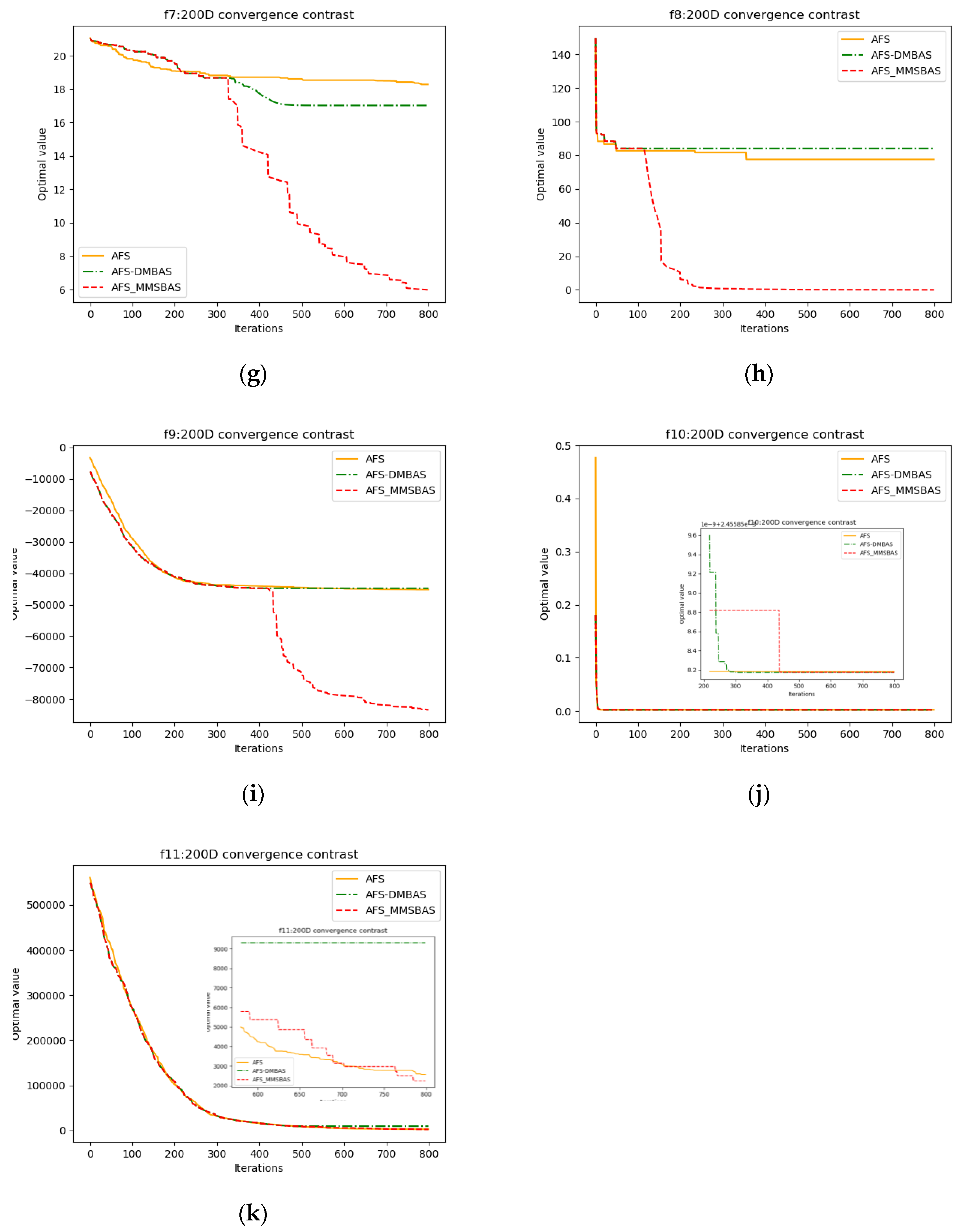
In order to solve the instability and low optimization accuracy at high dimensions of the AFS and BAS algorithms, this paper proposes a hybrid algorithm comprising the artificial fish swarm and beetle search algorithms (AFS-MMSBAS). The algorithm combines the advantages of the BAS and AFS, of which the BAS algorithm is improved by using the mutation of beetles and a multi-step detection strategy to improve optimization accuracy. In the early stage, the AFS algorithm is used for a global search and convergence to a certain extent; then, the improved BAS algorithm is used to accelerate convergence. The simulation results show that the AFS-MMSBAS algorithm has significantly improved stability and optimization compared with the AFS, MDBAS, and AFS-MDBAS algorithms.

2. Hybrid Algorithm of AFS and Improved BAS

To address the above problems, this section proposes the following algorithms:
(1)
Improved BAS algorithm: The use of the mutation strategy and the multi-step detection strategy of the BAS are proposed to allow the beetle to escape the local extremum value and accelerate convergence speed.
(2)
Hybrid of the AFS algorithm and BAS algorithm: The respective advantages of the AFS and BAS algorithms are combined to improve the optimization stability of the algorithm in high dimensions.

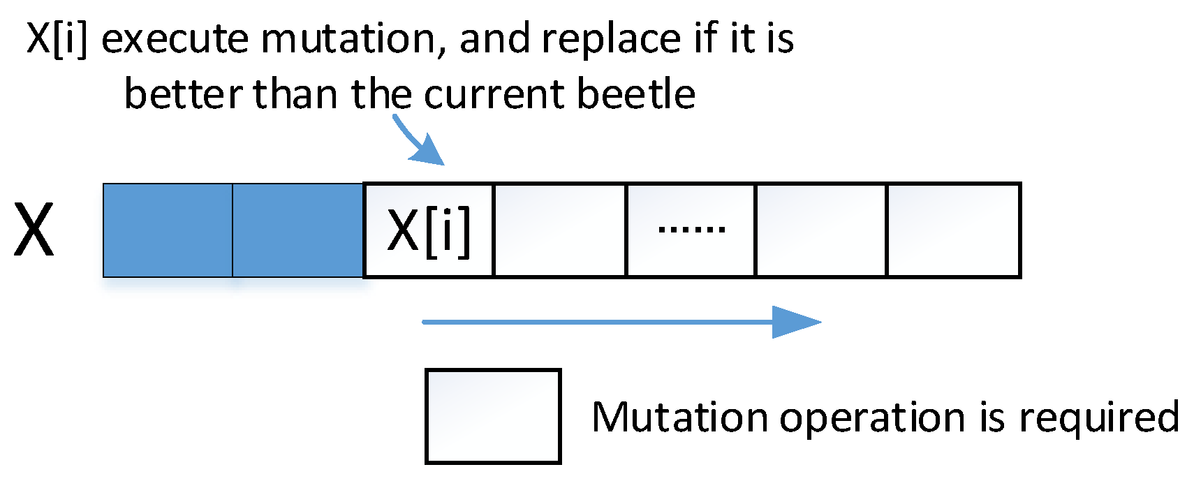
2.1. Mutation Selection Strategy of BAS

The BAS algorithm is prone to yielding values corresponding to a local extremum. In order to make the beetle escape a local extremum, the application of a mutation strategy to the beetle is proposed. In multi-dimensional problems, if each dimension changes at the same time, the following principle applies: the higher the dimension, the lower the probability that the newly generated individual is superior to the current individual. Therefore, this paper proposes a method wherein each dimension changes separately. If the beetle with the dimensional value changed is better than the one without a change, the current beetle will be updated. Otherwise, the mutation operation is continued in the next dimension—and so on—until the last dimension, as shown in Figure 1.
In addition, in order to acquire better results, a single variation is expanded to multiple variations. The beetle with the best fitness from multiple mutant beetles is selected, and the next step is initiated. The variation process is shown in Figure 2.

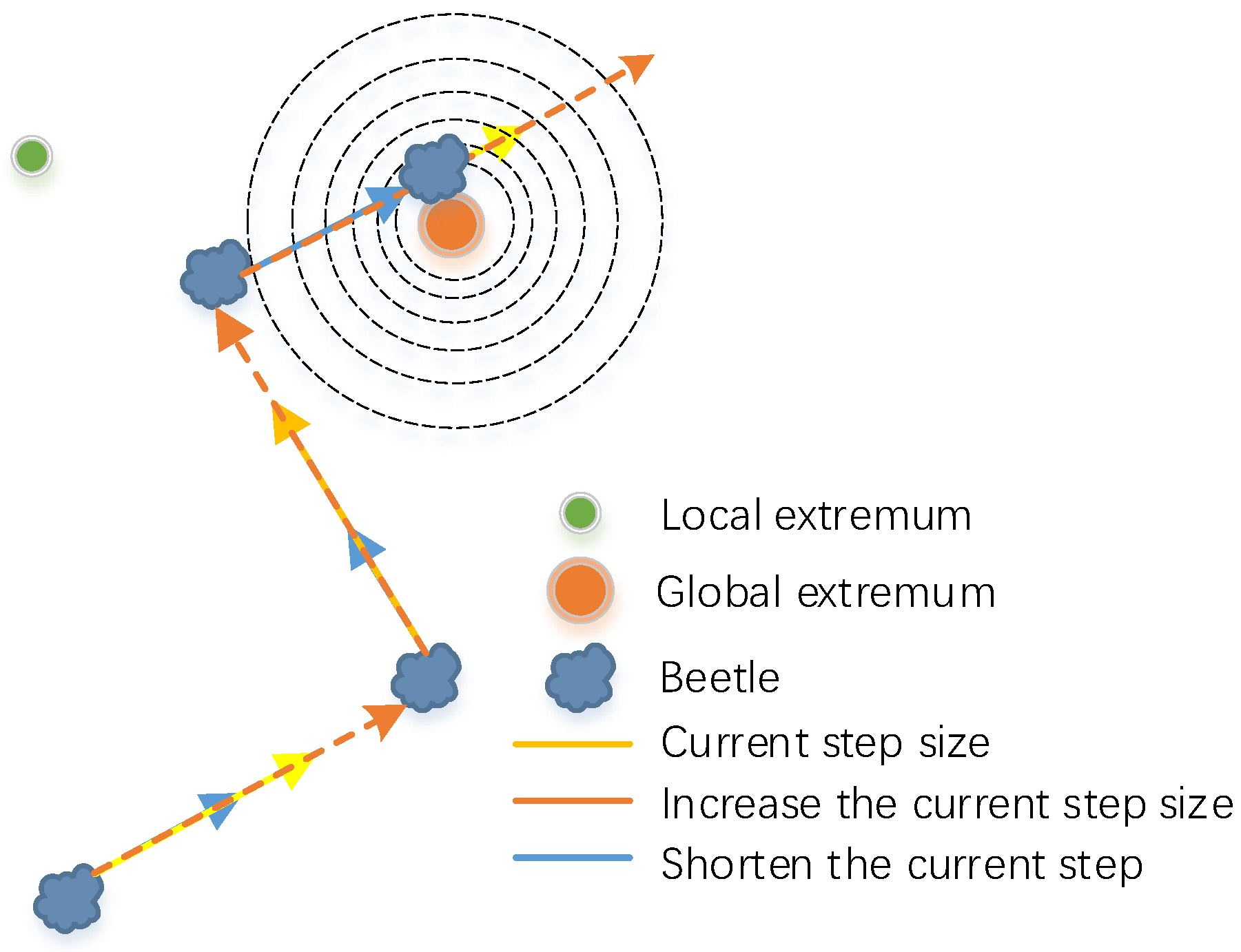
2.2. Multistep Detection Strategy

The choice of the initial step size has a great impact on the performance of the BAS algorithm. If the initial step size is too large, the algorithm converges slowly. If it is too small, it becomes easy to fall into the local extreme value and difficult to escape. The initial step size is usually determined manually and is then gradually reduced under the effect of a decreasing factor to achieve the goal of approaching the optimal value. Inspired by the multi-directional detection strategy [23], this paper proposes its own multi-step detection strategy. This strategy dynamically increases or decreases the step size in the optimization process and reduces the impact of the initial step size on the algorithm’s performance. The basic idea is to expand and reduce the current step size by a certain multiple, move forward according to different steps, and select the step size with the best fitness value for an update. This method can accelerate the convergence speed and increase the possibility of escaping local extremum. Figure 3 is a schematic diagram showing the multiple-step detection of the beetles.
Set the current iteration as i , the step size as s t e p i , and scale the step size according to Formula (1), where s t e p i ( ) represents the shortened step size, φ s is the reduction factor, s t e p i ( + ) represents the extended step size, and φ e is the amplification factor.
{ s t e p i ( ) = φ s s t e p i s t e p i ( + ) = φ e s t e p i
f ( x i , s ) is the fitness of the current beetle x i after a step length of s in a certain direction. Execute f ( x i , s t e p ) ,   f ( x i , s t e p i ( ) ) , and f ( x i , s t e p i ( + ) ) at the same time, and then select the step size corresponding to the optimal fitness s t e p b to update it according to Formula (2), where δ is the step-decreasing factor
s t e p i + 1 = s t e p b δ
Pseudocode of multi-step detection strategy is shown in Algorithm 1.
Algorithm 1. Multi-step detection pseudo code
1.
Inputs: step list = narrow _ step ,   s t e p ,   enlarge _ step
2.
for each  s t e p i of the step list do
3.
   f i t = f ( x , s t e p i )
4.
end for
5.
select s t e p b e s t of corresponding to the best f i t
6.
do Formula (2)
7.
return a new step
In addition, this paper initializes the step size of the beetle according to Formula (3) to avoid manual interference
s t e p = mean ( abs ( x ) ) / 3 + φ
wherein x represents the position of the initial beetle, δ represents the step-decreasing factor, and φ is a constant to prevent the initial step from equaling 0.

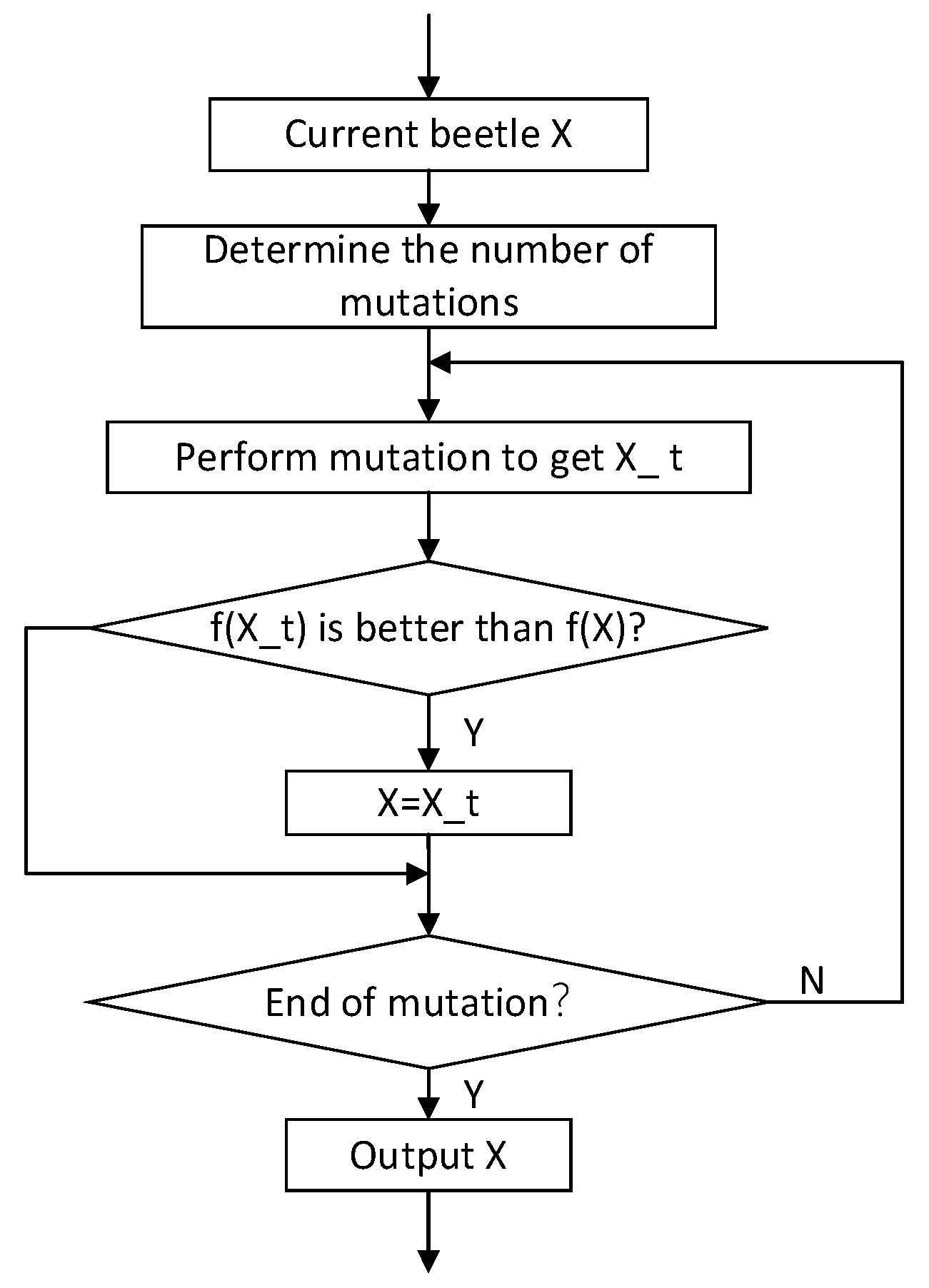
2.3. Hybrid Strategy of FAS-MMSBAS Algorithm

The FAS-MMSBAS algorithm is composed of the BAS algorithm and the AFS algorithm combined through a simple hybrid strategy. In the early stage, the AFS algorithm is used for global optimization and fast convergence, and in the later stage, the improved BAS algorithm is used to replace it and continue optimization. The hybrid algorithm reduces the instability of the BAS algorithm caused by individual random initialization to a certain extent, accelerates the convergence speed, and improves the optimization accuracy. The most important consideration regarding the hybrid algorithm is to determine when to end the AFS algorithm. If it is too early, the global optimization ability of the AFS algorithm will be too small. If it is too late, it will converge too slowly and waste time. Therefore, according to the characteristics of the AFS algorithm, this paper proposes the termination of the AFS algorithm when the optimal value remains unchanged or the convergence speed becomes significantly slow. The optimal individual obtained by the AFS algorithm is taken as the initial individual of the BAS algorithm. The interruption rule of the AFS algorithm is shown in Algorithm 2:
Algorithm 2. FAS algorithm termination rule pseudo code
1.
Input: parameters p and q
2.
if the repeat times of best individual == q, or maximum iterations of AFS > q then
3.
  initial individual of the BAS = The optimal individual of AFS
4.
end if
5.
do Improve BAS
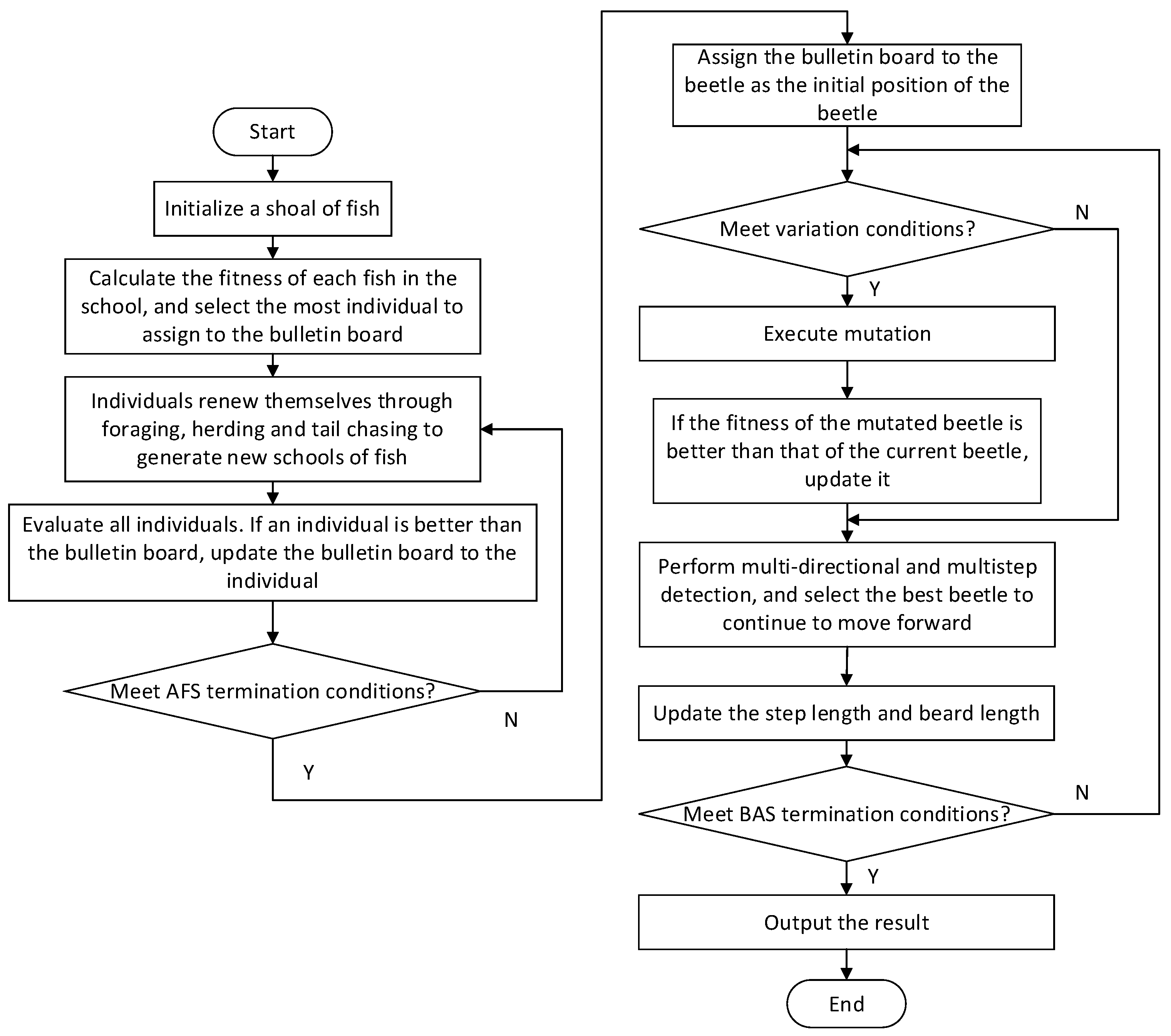
The parameters p and q are manually set values, where p represents the number of iterations of the best value, and q represents the maximum number of iterations of the AFS algorithm in the hybrid algorithm. When the fish swarm iterates p times and the optimal position remains unchanged, the AFS algorithm ends. This means that the current fish population may find the best value or fall into a local extreme value. In addition, because the AFS algorithm converges slowly in the later period, if condition p is not met under certain conditions, q is set as the termination condition of the AFS algorithm to avoid wasting time. The implementation steps of FAS-MMSBAS algorithm are as follows:
Step 1. Set the initial parameters of the algorithm, including the populations, visual properties, attempt number, crowding factor, steps of the fish, antenna number, antenna length, and variation rate.
Step 2. Use the AFS algorithm to continuously optimize until the AFS iteration termination condition is met.
Step 3. Take the best individual in the optimization stage of the AFS algorithm as the initial position for the optimization of the beetle.
Step 4. Judge whether there is variation. If there is, go to step 5; if not, go to step 6.
Step 5. Allow the dimension to be mutated, until the end of the mutation.
Step 6. Perform multi-directional and multistep detection on the beetle; then, select the best beetle to continue to move forward and update the current beetle step length and whisker length.
Step 7. If the termination conditions are met, the algorithm is ended; if not, go to step 4.
Figure 4 provides a flow chart of the AFS-MMSBAS algorithm depicted according to the above steps.

3. Results and Analysis

3.1. Test Function and Evaluation Indicator

In order to verify the performance of the hybrid algorithm proposed in this paper, 11 typical test functions are selected for simulation experiments, as shown in Table 1, including the function name, search range, optimal position, and optimal value. In addition, Table 2 is a supplement to Table 1, which is used to show function expressions. f 1 ~ f 4 are unimodal functions, which are used to test the optimization ability of the algorithm for a single extreme value function. f 5 ~ f 10 are multimodal functions, which are used to test the global search ability of the algorithm under multiple local extreme values and the ability to solve complex optimization problems. f 2 and f 10 are non-partitioned functions with a control relationship between dimensions; f 4 is a noise function with random interference; and f 11 is a step function.
Three indicators are selected in the experiment to evaluate the performance of the algorithm:
(1)
The mean, which is the average value of the algorithm run many times, reflecting the quality of the solution. The closer the average value is to the optimal value, the better the algorithm’s results.
(2)
The standard deviation, which is the standard deviation of the optimal value and can reflect the stability of the algorithm. The smaller the standard deviation, the better the stability of the algorithm.
(3)
The running time, in seconds, which is the average time of multiple runs of the algorithm under the same environment and parameters, reflecting the running efficiency of the algorithm.
The calculation formulas of the three evaluation indicators are shown in Formulas (4)–(6):
Mean = | 1 N i = 1 n f ( x i ) |
Standard = 1 N i n ( f ( x i ) M e a n ) 2
Time = 1 N i n t i

3.2. Computational Complexity Analysis of FAS-MMSBAS Algorithm

The main improvement to the algorithms in this paper is that after the convergence of the AFS algorithm becomes slow, the improved BAS algorithm is used to continue to search for the optimal position. In the later stage, the optimization is changed from population optimization to individual optimization, which reduces the complexity of the algorithm. When the optimization problem dimension is D and the population number is N, the complexity analysis of the FAS-MMSBAS algorithm is as follows: the number of iterations of the AFS algorithm is t1, the number of iterations of the MMSBAS algorithm is t2, and the total number of iterations is T = t1 + t2. In the optimization stage of the AFS algorithm, the computational complexity of initializing the artificial fish group is O(DN). In the iteration process, the computational complexity of clustering behavior is O(DN2), and that of chasing behavior is O(DN2); thus, the total complexity of this stage is O(DN) + O(2DN2)t1. In the iteration process of the MMSBAS algorithm, the number of multi-directional detection is c1, the number of multi-step detection is 3, the computational complexity of the multi-directional multistep detection strategy is O(3c1D), the computational complexity of the mutation strategy is O(D), and the total computational complexity is O(c2D)t2, c1 < c2. Combined with the two stages, the total computational complexity of the algorithm can be approximated as O(DN2)t1 + O(c2D)t2.
It can be seen from Table 3 that when the number of iterations is the same, the order of algorithm complexity from low to high is BAS < AFS-DBAS < AFS-MMBAS < AFS.

3.3. Simulation Experiment and Result Analysis

The algorithms’ comparison and analysis are arranged as follows: (1) first, compare AFS-MMSBAS algorithm with two basic algorithms and the hybrid algorithm of the basic algorithm based on different dimensions; (2) further analyze the stability and convergence speed of the AFS-MMSBAS algorithm in high dimensions; and (3) compare the performance of the AFS-MMSBAS algorithm and other related algorithms in high dimensions.

3.3.1. Parameter Setting

The relevant parameter settings with which to avoid the influence of different parameters on the algorithm are shown in Table 4. All experiments in this paper are based on the PyCharm platform and were run on the Window10 (64 bit) operating system with the processor configured as Inter (R) Core (TM) i5-5200U CPU @ 2.20GHz 2.20 GHz with a memory of 12 GB.

3.3.2. Performance Comparison in Different Dimensions

The AFS-MMSBAS algorithm is compared with the MDBAS, AFS, and AFS-MDBAS algorithms under the same parameters. The performance of the algorithms is tested with respect to the dimensions D = 10, D = 100, and D = 200 of the basic test functions. In order to prevent the experimental results from being affected by randomness, each test function is independently run 50 times. The other parameters are the same as those in 3.2.1. Finally, the average value, standard deviation, and running time of the optimization results are obtained. The experimental results are shown in Table 5, and the optimal results are shown in bold.
By analyzing Table 2, it can be seen that in low dimensions (D = 10), the MDBAS, AFS, AFS-MDBAS, and AFS-MMSBAS algorithms have good optimization ability and stability for most test functions. Among them, the MDBAS algorithm obtains the optimal mean and standard deviation for f 5 , the AFS algorithm obtains the optimal mean and standard deviation for f 2 and f 11 , the AFS-MDBAS algorithm obtains the optimal mean and standard deviation for f 3 and f 10 , and the AFS-MMSBAS algorithm obtains the optimal mean and standard deviation for f 1 , f 4 , f 8 , and f 9 . At low dimensions, each algorithm has certain advantages over different functions, and the gap is not obvious.
At high dimensions (D = 100, 200), the averages of the MDBAS algorithm and the AFS algorithm are far greater than the optimal value, and the standard deviation is also large, indicating that the optimization ability and stability of these two algorithms are poor. For most functions, the averages and standard deviations of the AFS-MDBAS hybrid algorithm are better than those of the separate MDBAS and AFS algorithms, which shows that the hybrid algorithm improves the optimization ability and stability of the MDBAS and AFS algorithms. The AFS-MMSBAS algorithm is an improvement of the AFS-MDBAS algorithm. Although the algorithm is not the best at optimizing the functions f7, f9, f10, and f11, it is not far behind the algorithm with the best performance. In general, the AFS-MMSBAS algorithm proposed in this paper has better optimization ability and stability with respect to high-dimensional problems.
Finally, under the same number of iterations, it can be seen that the running time of the algorithm increases with the increase in dimensions. Moreover, whether at low or high dimensions, the hybrid algorithm greatly shortens the running time compared with the AFS algorithm. However, compared with the BAS algorithm, it greatly increases the running time. The hybrid algorithm trades time for optimization capability and stability. The running time relationship between algorithms is as follows: T (MDBAS) < T (AFS-MDBAS) < T (AFS-MMSBAS) < T (AFS).

3.3.3. Stability Analysis of Algorithms

In order to observe and compare the stability of each algorithm at higher dimensions more intuitively, functions f 1 ~ f 11 are run 50 times in order to develop line graphs (D = 200), as shown in Figure 5a–k. The more stable the curve, the better the stability of the algorithm. The smaller the value of the curve, the better the optimization ability of the algorithm.
For unimodal functions f 1 ~ f 4 , the fluctuation of the MDBAS algorithm (blue) and the AFS algorithm (orange) is large, and the curve is far from the optimal value. Combined with Table 5, it can be seen that the stability and optimization accuracy of the AFS-MDBAS (green) and AFS-MMSBAS algorithm (red) are better than those of the individual algorithms. This shows that the hybrid algorithm composed of the AFS and BAS algorithms achieves superior performance for unimodal functions. For the multimodal functions f 5 ~ f 10 , the advantages of the AFS-MDBAS algorithm in terms of stability and optimization accuracy are not obvious compared with the AFS and MDBAS algorithms, but the advantages of the AFS-MMSBAS algorithm are quite obvious. The curve is the most stable and is below all the other curves, which further demonstrates that the AFS-MMSBAS algorithm has the best stability and optimization ability.

3.3.4. Analysis of the Convergence of the Algorithm

To observe the convergence of the improved BAS algorithm at high dimensions, the convergence curve of functions f 1 ~ f 11 when D = 200 is developed, as shown in Figure 6a–k. It can be seen from the figure that the convergence curves of the three algorithms are basically coincident in the early stage. Since the AFS algorithm is used for optimization at this stage, the degree of convergence is basically the same. In the later stage, except for functions f 10 and f 11 , the convergence curve of the AFS-MMSBAS algorithm drops faster than that of the AFS-DMBAS and AFS algorithms. This shows that the improved BAS algorithm has better convergence speed than the MDBAS algorithm. In addition, the convergence curve of the AFS-MMSBAS algorithm is lower than those of the other algorithms, which also shows that the optimization ability of the algorithm is better than that of the AFS-MDBAS and AFS algorithms.

3.3.5. Comparison with Other Algorithms

The above experiments verify that the stability and optimization ability of the AFS-MMSBAS algorithm are better than the two basic algorithms with respect to high-dimensional problems. This section compares the AFS-MMSBAS algorithm with other related algorithms, an Adaptive Dual-Strategy AFS algorithm based on the PSO algorithm (ADSAFS-PSO) [16], and an Adaptive AFSA utilizing Gene Exchange (AAFSA-GE) [17]. The unimodal function f 1 , noise function f 4 , multimodal functions f 5 and f 8 , non-partitioned function f 10 , and step function f 11 are selected as test functions. The parameter settings are as follows: population 50, crowding factor 0.75, attempt number = 5, dimensions D = 10 and D = 200, and iterations 800. The other relevant parameters of the AFS-MMABAS algorithm are the same as those in Section 3.3.1, and the other parameters of the PSOEM-FSA and AAFSA-GE algorithms are the same as those in the references. Each algorithm runs independently 10 times. The experimental results are shown in Table 6, including the average, standard deviation, the maximum and minimum of the optimization results, and the average running time of the algorithm.
As seen from the table, at low dimensions, the three algorithms can converge to the minimum value for functions f 5 and f 11 , but the ADSAFS-PSO algorithm is more stable. Moreover, the average value and standard deviation index obtained by the ADSAFS-PSO algorithm are also better than the other two algorithms. In general, the AAFSA-GE algorithm has the best optimization accuracy and stability at low dimensions, while the AFS-MMSBAS and ADSAFS-PSO algorithms perform similarly. However, at high dimensions, the average, standard deviation, and maximum index obtained by the AFS-MMSBAS algorithm are superior to the other two algorithms. Therefore, the AFS-MMSBAS algorithm has more advantages than the other algorithms. However, although the AFS-MMSBAS algorithm has good optimization performance for most test functions, it has poor optimization performance for f11 functions. This shows that the algorithm is not suitable for the optimization of step functions.
In addition, the running time of the AFS-MMSBAS algorithm is the shortest.

4. Conclusions

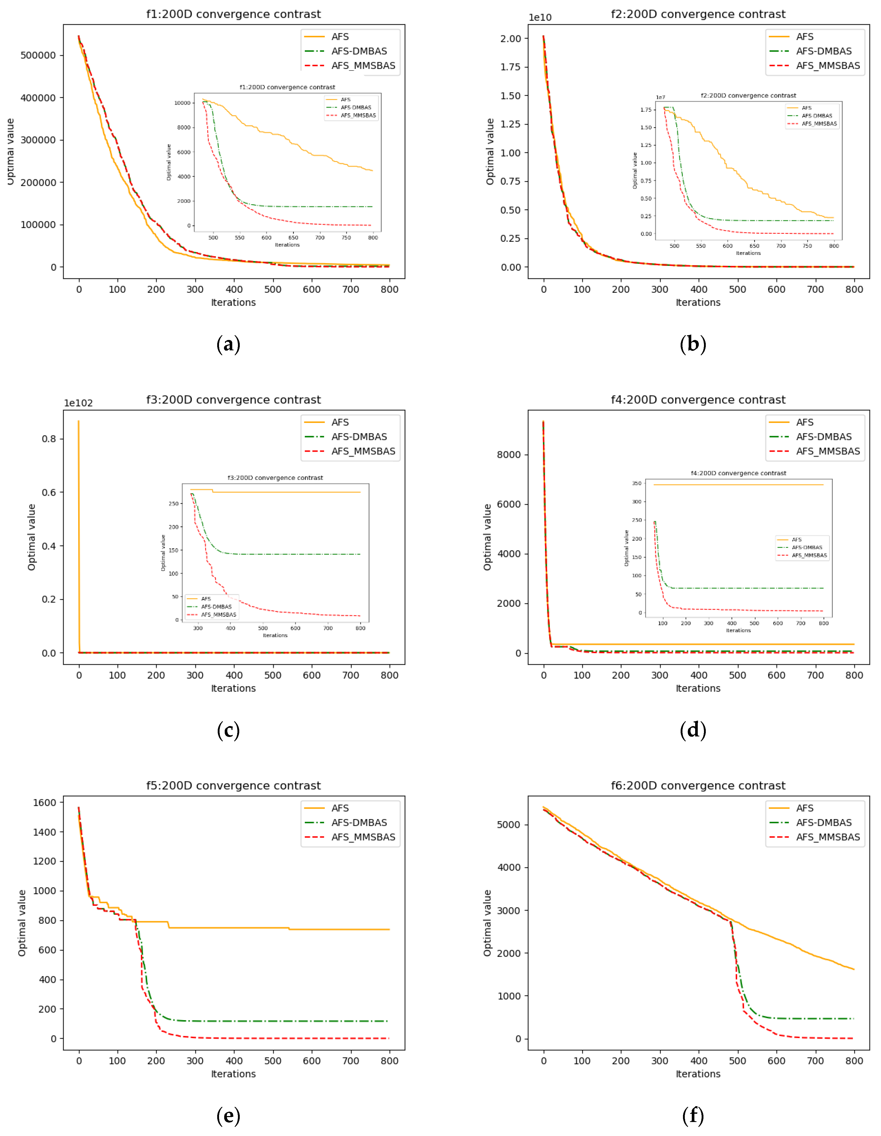
In view of the advantages and disadvantages of the AFS algorithm and BAS algorithm, this paper proposes a hybrid algorithm, AFS-MMSBAS, which combines the artificial fish swarm and improved beetle antenna search algorithms. This hybrid algorithm involves the use of a mutation strategy to increase the probability of a beetle escaping the local extreme value and altering its course to a better direction. It also proposes a multi-step detection strategy to improve the convergence speed of the algorithm by adaptively changing the step size. Finally, a simple method is used to combine the AFS algorithm with the improved BAS algorithm. In order to test that the AFS-MMSBAS algorithm is superior to its two constituent algorithms, the AFS-MMSBAS algorithm is compared with the AFS, BAS, and AFS-BAS algorithms at different dimensions. In order to further verify the advantages of this algorithm in dealing with high-dimensional problems, the AFS-MMSBAS algorithm is compared with similar algorithms, namely, AAFSA-GE and ADSAFS-PSO. The experimental results show that the AFS-MMSBAS algorithm can solve the problems of the poor optimization and instability of the AFS and BAS algorithms at high dimensions, and that it has a faster convergence speed during the later period. In a word, the AFS-MMSBAS algorithm performs well in high-dimensional problem processing.
The algorithm proposed in this paper performs well for high-dimensional problem optimization but performs poorly for some function problems, such as step functions. In addition, the algorithm has poor ability to solve low-dimensional problems and has great room for improvement. Therefore, in the future work, the authors plan to improve the algorithm, specifically with respect to its ability to solve high-dimensional partial function optimization and deal with low-dimensional problems. Further, it will be applied to engineering practices.

Author Contributions

J.N. and J.T. proposed the idea of the paper. J.T. and R.W. helped manage the annotation group and helped clean the raw annotations. J.T. conducted all experiments and wrote the manuscript. J.N., J.T. and R.W. revised and improved the text. J.N. and J.T. are the people in charge of this project. All authors have read and agreed to the published version of the manuscript.

Funding

This work was supported by the Handan Science and Technology Research and Development Program (19422091008-35) and the Hebei Science and Technology Program (21350101D).

Institutional Review Board Statement

Not applicable.

Informed Consent Statement

Not applicable.

Data Availability Statement

Not applicable.

Conflicts of Interest

The authors declare no conflict of interest.

References

  1. Rahkar Farshi, T. Battle Royale Optimization Algorithm. Neural Comput. Appl. 2021, 33, 1139–1157. [Google Scholar] [CrossRef]
  2. Ghafil, H.N.; Jármai, K. Dynamic Differential Annealed Optimization: New Metaheuristic Optimization Algorithm for Engineering Applications. Appl. Soft Comput. 2020, 93, 106392. [Google Scholar] [CrossRef]
  3. Nadimi-Shahraki, M.H.; Fatahi, A.; Zamani, H.; Mirjalili, S.; Abualigah, L. An Improved Moth-Flame Optimization Algorithm with Adaptation Mechanism to Solve Numerical and Mechanical Engineering Problems. Entropy 2021, 23, 1637. [Google Scholar] [CrossRef] [PubMed]
  4. Yuan, Z.; Wang, W.; Wang, H.; Razmjooy, N. A New Technique for Optimal Estimation of the Circuit-Based PEMFCs Using Developed Sunflower Optimization Algorithm. Energy Rep. 2020, 6, 662–671. [Google Scholar] [CrossRef]
  5. Abdel-Basset, M.; Chang, V.; Mohamed, R. A Novel Equilibrium Optimization Algorithm for Multi-Thresholding Image Segmentation Problems. Neural Comput. Appl. 2021, 33, 10685–10718. [Google Scholar] [CrossRef]
  6. Gao, Y.; Yang, Q.; Wang, X.; Li, J.; Song, Y. Overview of new swarm intelligence optimization algorithms. J. Zhengzhou Univ. (Eng. Ed.) 2022, 43, 21–30. [Google Scholar]
  7. Yang, X.-S.; Deb, S. Cuckoo Search via Lévy Flights. In Proceedings of the 2009 World Congress on Nature & Biologically Inspired Computing (NaBIC), Coimbatore, India, 9–11 December 2009; IEEE: Piscataway, NJ, USA, 2009; pp. 210–214. [Google Scholar] [CrossRef]
  8. Wang, D.; Tan, D.; Liu, L. Particle Swarm Optimization Algorithm: An Overview. Soft Comput. 2018, 22, 387–408. [Google Scholar] [CrossRef]
  9. Xia, X.; Zhou, Y. Research progress of ant colony optimization algorithm. J. Intell. Syst. 2016, 11, 10. [Google Scholar]
  10. Cheng, M.; Ni, Z.; Zhu, X. Overview of Firefly Optimization Algorithm. Theory computer science. 2015, 42, 19–24. [Google Scholar]
  11. Bastos Filho, C.J.A.; de Lima Neto, F.B.; Lins, A.J.C.C.; Nascimento, A.I.S.; Lima, M.P. A Novel Search Algorithm Based on Fish School Behavior. In Proceedings of the 2008 IEEE International Conference on Systems, Man and Cybernetics, Singapore, 12–15 October 2008; pp. 2646–2651. [Google Scholar]
  12. Zhang, L.; Fu, M.; Fei, T.; Li, H. The Artificial Fish Swarm Algorithm Improved by Fireworks Algorithm. Autom. Control. Comput. Sci. 2022, 56, 11–323. [Google Scholar]
  13. Zhang, C.; Zhang, F.; Li, F.; Wu, H. Improved Artificial Fish Swarm Algorithm. In Proceedings of the 2014 9th IEEE Conference on Industrial Electronics and Applications, Hangzhou, China, 9–11 June 2014; pp. 748–753. [Google Scholar]
  14. Liu, D.; Li, L. A novel improved artificial fish swarm algorithm. Comput. Sci. 2017, 44, 281–287. [Google Scholar]
  15. Li, J.; Liang, X.M. Improved artificial fish swarm algorithm for elite acceleration. Comput. Appl. Res. 2018, 35, 1960–1964+1981. [Google Scholar]
  16. Liu, Z.; Shu, Z.; Xu, Y.; Yang, S.; Shen, W. Artificial fish swarm algorithm based on PSO adaptive dual strategy. Comput. Mod. 2022, 5, 46–53. [Google Scholar]
  17. Li, Z.; Zhou, K.; Ou, Y.; Ding, L. Adaptive artificial fish swarm algorithm based on gene exchange. Comput. Appl. 2022, 42, 701–707. [Google Scholar]
  18. Jiang, X.; Li, S. BAS: Beetle Antennae Search Algorithm for Optimization Problems. Int. J. Robot. Control 2017, 1, 1. [Google Scholar] [CrossRef]
  19. Zivkovic, M.; Bacanin, N.; Venkatachalam, K.; Nayyar, A.; Djordjevic, A.; Strumberger, I.; Al-Turjman, F. COVID-19 Cases Prediction by Using Hybrid Machine Learning and Beetle Antennae Search Approach. Sustain. Cities Soc. 2021, 66, 102669. [Google Scholar] [CrossRef] [PubMed]
  20. Huang, J.; Duan, T.; Zhang, Y.; Liu, J.; Zhang, J.; Lei, Y. Predicting the Permeability of Pervious Concrete Based on the Beetle Antennae Search Algorithm and Random Forest Model. Adv. Civ. Eng. 2020, 2020, 8863181. [Google Scholar] [CrossRef]
  21. Xiang, Q.; Zhu, P. Image Denoising Using a Deep Auto-Encoder Approach Based on Beetle Antennae Search Algorithm. In Computer and Communication Engineering; Neri, F., Du, K.-L., Varadarajan, V.K., Angel-Antonio, S.-B., Jiang, Z., Eds.; Springer International Publishing: Cham, Switzerland, 2022; Volume 1630, pp. 75–84. [Google Scholar]
  22. Wang, J.; Chen, H. BSAS: Beetle Swarm Antennae Search Algorithm for Optimization Problems. arXiv 2018, arXiv:1807.10470. [Google Scholar]
  23. Zhao, Y.; Qian, Q.; Zhou, T. Fuyun sends A hybrid algorithm of longicorn beetle whisker search and genetic algorithm. Minicomput. Sys. 2020, 41, 8. [Google Scholar]
  24. Khan, A.H.; Cao, X.; Li, S.; Katsikis, V.N.; Liao, L. BAS-ADAM: An ADAM Based Approach to Improve the Performance of Beetle Antennae Search Optimizer. IEEE/CAA J. Autom. Sin. 2020, 7, 461–471. [Google Scholar] [CrossRef]
Figure 1. Variation diagram of single beetle in high-dimensional case.
Applsci 12 13044 g001
Figure 2. Flow chart of variation.
Applsci 12 13044 g002
Figure 3. Schematic diagram of multi-step detection.
Applsci 12 13044 g003
Figure 4. Flow chart of FAS-MMSBAS algorithm.
Applsci 12 13044 g004
Figure 5. D = 200; comparison of stability of functions f 1 ~ f 11 . (a) Comparison of stability of four algorithms for function f 1 ; (b) Comparison of stability of four algorithms for function f 2 ; (c) Comparison of stability of four algorithms for function f 3 ; (d) Comparison of stability of four algorithms for function f 4 ; (e) Comparison of stability of four algorithms for function f 5 ; (f) Comparison of stability of four algorithms for function f 6 ; (g) Comparison of stability of four algorithms for function f 7 ; (h) Comparison of stability of four algorithms for function f 8 ; (i) Comparison of stability of four algorithms for function f 9 ; (j) Comparison of stability of four algorithms for function f 10 ; (k) Comparison of stability of four algorithms for function f 11 .
Applsci 12 13044 g005aApplsci 12 13044 g005bApplsci 12 13044 g005c
Figure 6. D = 200, functions f 1 ~ f 11 convergence performance. (a) Comparison of convergence of three algorithms for function f 1 ; (b) Comparison of convergence of three algorithms for function f 2 ; (c) Comparison of convergence of three algorithms for function f 3 ; (d) Comparison of convergence of three algorithms for function f 4 ; (e) Comparison of convergence of three algorithms for function f 5 ; (f) Comparison of convergence of three algorithms for function f 6 ; (g) Comparison of convergence of three algorithms for function f 7 ; (h) Comparison of convergence of three algorithms for function f 8 ; (i) Comparison of convergence of three algorithms for function f 9 ; (j) Comparison of convergence of three algorithms for function f 10 ; (k) Comparison of convergence of three algorithms for function f 11 .
Applsci 12 13044 g006aApplsci 12 13044 g006b
Table 1. Benchmark test functions.
FunctionFunction NameSearch RangeOptimal PositionOptimum Value
f 1 Sphere x i ϵ [ 100 , 100 ] (0,0,…,0)0
f 2 Rosenbrock x i ϵ [ 50 , 50 ] (1,1,…,1)0
f 3 SchwefelP222 x i ϵ [ 10 , 10 ] (0,0,…,0)0
f 4 Quartic x i ϵ [ 1.28 , 1.28 ] (0,0,…,0)0
f 5 Rastrigin x i ϵ [ 5.12 , 5.12 ] (0,0,…,0)0
f 6 Griewank x i ϵ [ 600 , 600 ] (0,0,…,0)0
f 7 Ackley x i ϵ [ 32 , 32 ] (0,0,…,0)0
f 8 Levy and Montalvo 2 x i ϵ [ 5 , 5 ] (1,1,…,1)0
f 9 Schwefel226 x i ϵ [ 500 , 500 ] (420.968746, …, 420.968746)−418.98288 × D
f 10 Schaffer x i ϵ [ 100 , 100 ] (0,0,…,0)0
f 11 Step x i ϵ [ 100 , 100 ] (0,0,…,0)0
Table 2. Expressions of benchmark test function; this table is a supplement to Table 1.
Function NameExpression
Sphere f 1 = i = 1 D x i 2
Rosenbrock f 2 = i = 1 D 1 [ 100 ( x i + 1 x i 2 ) 2 + ( x i 1 ) 2 ]
SchwefelP222 f 3 = i = 1 D | x i | + i = 1 D | x i |
Quartic f 4 = i = 1 D ( i x i 4 ) + r a n d o m [ 0 , 1 )
Rastrigin f 5 = i = 1 D [ x i 2 10 cos ( 2 π x i ) + 10 ]
Griewank f 6 = 1 4000 i = 1 D x i 2 i = 1 D [ c o s ( x i i ) ] + 1
Ackley f 7 = 20 e x p ( 0.2 1 D i = 1 D x i 2 ) e x p ( 1 D i = 1 D c o s ( 2 π x i ) ) + 20 + e
Levy and Montalvo 2 f 8 = 0.1 { s i n 2 ( 3 π x 1 ) + i = 1 D ( x i 1 ) 2 [ 1 + s i n 2 ( 3 π x i + 1 ) ] + ( x D 1 ) 2 [ 1 + s i n 2 ( 2 π x D ) ] }
Schwefel226 f 9 = i = 1 D x i s i n ( | x i | )
Schaffer f 11 = i = 1 D 1 ( x i 2 + x i + 1 2 ) 0.25 [ s i n 2 ( 50 ( x i 2 + x i + 1 2 ) 0.1 ) + 1 ]
Step f 10 = i = 1 D ( f l o o r ( x i + 0.5 ) ) 2
Table 3. Algorithm complexity.
AlgorithmCalculation ComplexityAlgorithmCalculation Complexity
AFSO(DN2) TAFS-DBASO(DN2)t1 + O(c1D)t2
BASO(D) TAFS-MMBASO(DN2)t1 + O(c2D)t2
Table 4. Initial parameters of AFS-MMSBAS algorithm.
ParameterValueParameterValue
population30antenna number10
visual6antenna lengthstep/5
attempt number20 δ 0.95
crowding factor0.618variation rate0.05
step of fish0.6p40
iterations800q0.65 × iterations
Table 5. Comparisons of four algorithms regarding the optimization of test functions f 1 ~ f 11  .
Func.AlgorithmD = 10D = 100D = 200
MeanStandardTimeMeanStandardTimeMeanStandardTime
f 1 MDBAS4.5 × 10−321.91 × 10−321.0089.16 × 1023.98 × 1023.4814.91 × 1047.16 × 1037.045
AFS0.6270.15494.873.08 × 10251.4149.84.43 × 1035.14 × 102213.4
AFS-MDBAS8.37 × 10−282.28 × 10−2713.257.513.6468.922.0 × 1032.99 × 10282.17
AFS-MMSBAS4.5 × 10−1064.99 × 10−10517.270.008140.0045472.9719.14.6781.85
f 2 MDBAS4.62 × 1029.69 × 1021.3413.92 × 1064.23 × 1064.9115.21 × 1081.58 × 1087.65
AFS67.318.6105.53.57 × 1042.29 × 104166.41.84 × 1063.99 × 105253.7
AFS-MDBAS1.25 × 1023.12 × 1024.461.74 × 1031.23 × 10383.171.58 × 1066.05 × 105130.7
AFS-MMSBAS90.23.22 × 1028.0714.08 × 1023.99 × 10286.125.18 × 1031.69 × 103133.7
f 3 MDBAS0.06590.4541.3333.19 × 1092.25 × 10104.9791.94 × 10377.36 × 10377.355
AFS2.010.345131.91.32 × 1023.56130.12.67 × 1025.52180.0
AFS-MDBAS4.99 × 10−141.26 × 10−1315.7138.14.9323.631.41 × 1029.8532.26
AFS-MMSBAS0.09250.082329.392.740.9232.3310.32.1942.11
f 4 MDBAS0.1950.1181.56123.34.84.9582.59 × 10248.07.638
AFS0.3880.142134.571.118.5176.73.21 × 10281.9317.8
AFS-MDBAS0.1960.09869.23913.63.4715.2464.111.528.59
AFS-MMSBAS0.03610.024413.041.180.31120.113.430.742.35
f 5 MDBAS2.56 × 10−152.07 × 10−151.2412.381.334.921.27 × 10219.47.058
AFS0.5440.141126.21.81 × 10222.2189.46.46 × 10250.9332.4
AFS-MDBAS2.98 × 10−152.34 × 10−1519.61.870.9743.931.2 × 10217.599.94
AFS-MMSBAS2.66 × 10−153.17 × 10−1528.563.45 × 10−86.32 × 10−847.260.002360.00541108.7
f 6 MDBAS0.05650.03911.8658.984.354.2284.58 × 10262.18.403
AFS0.1820.028564.831.43 × 1021.0 × 10241.341.48 × 10379.360.52
AFS-MDBAS0.1040.069520.437.162.9525.744.48 × 10261.840.41
AFS-MMSBAS0.09820.057928.480.3350.092827.92.20.60147.5
f 7 MDBAS0.2790.6661.66318.30.3394.34619.10.188.062
AFS2.370.234153.112.60.327248.017.90.276321.0
AFS-MDBAS0.250.61219.0411.10.90274.8718.10.52992.61
AFS-MMSBAS0.480.59423.024.220.77886.454.240.7109.0
f 8 MDBAS0.07930.1481.6152.140.9195.30411.61.748.444
AFS0.1940.0669104.631.41.1137.778.42.25241.9
AFS- MDBAS0.02220.039212.6916.512.721.9175.57.3328.76
AFS-MMSBAS0.001540.002616.620.002940.0036529.290.01110.0073548.42
f 9 MDBAS−2.35 × 1033.84 × 1021.136−2.03 × 1041.15 × 1034.789−3.57 × 1041.67 × 1037.777
AFS−3.11 × 1032.59 × 102119.6−2.45 × 1044.59 × 102201.1−4.66 × 1049.21 × 102311.3
AFS- MDBAS−2.4 × 1033.64 × 10213.19−2.51 × 1047.1 × 10296.28−4.68 × 1049.3 × 102169.5
AFS-MMSBAS−4.18 × 10320.815.8−4.12 × 1045.55 × 102104.99−8.01 × 1041.84 × 103177.2
f 10 MDBAS0.07780.06913.5820.1720.16411.010.2790.16219.64
AFS0.002461.33 × 10−10253.90.002462.02 × 10−10591.50.002461.75 × 10−10888.0
AFS- MDBAS0.002462.85 × 10−1724.410.002462.76 × 10−1789.420.002462.98 × 10−17109.7
AFS-MMSBAS0.002464.56 × 10−927.20.002461.71 × 10−1095.40.002464.87 × 10−11149.5
f 11 MDBAS3.682.612.8691.37 × 1043.45 × 10313.191.11 × 1051.55 × 10428.22
AFS0.00.0236.728.824.2397.23.31 × 1034.71 × 102617.4
AFS- MDBAS0.480.70718.455.48 × 1021.45 × 10254.519.63 × 1039.6 × 102225.1
AFS-MMSBAS0.060.2421.121.87 × 10257.761.782.08 × 1037.05 × 102271.2
Table 6. Comparison between AFS-MMSBAS algorithm and other similar algorithms.
Func.AlgorithmD = 10D = 200
MeanStandardMinMaxTimeMeanStandardMinMaxTime
f 1 ADSAFS-PSO8.88 × 10−172.15 × 10−1606.66 × 10−16248.23.14 × 1037.39 × 10310.42.29 × 104589.4
AAFSA-GE1.81 × 10−1473.54 × 10−1476.81 × 10−1481.81 × 10−146186.41.9 × 1032.44 × 1038.58.31 × 103428.1
AFS-MMSBAS2.73 × 10−1088.26 × 10−1083.17 × 10−1182.62 × 10−10765.9725.57.6414.235.7268.7
f 4 ADSAFS-PSO9.25 × 10−51.21 × 10−46.27 × 10−64.21 × 10−6300.342.098.83.053.2 × 102499.4
AAFSA-GE5.08 × 10−631.02 × 10−611.8 × 10−646.52 × 10−61242.35.142.470.4110.4314.2
AFS-MMSBAS0.04630.03810.007540.13439.393.660.6032.744.5188.24
f 5 ADSAFS-PSO3.55 × 10−161.12 × 10−1503.55 × 10−15293.063.739.616.01.32 × 102462.2
AAFSA-GE0000184.33.2 × 10−23.74 × 10−24.12 × 10−39.04 × 10−2341.5
AFS-MMSBAS2.31 × 10−151.88 × 10−1505.33 × 10−1557.498.01 × 10−48.37 × 10−41.89 × 10−43.04 × 10−3190.6
f 8 ADSAFS-PSO0.08450.1231.55 × 10−150.274323.932.49.221.747.3515.2
AAFSA-GE2.48 × 10−101.28 × 10−64.9 × 10−114.9 × 10−9203.13. 252.41.656.7396.2
AFS-MMSBAS0.002310.002976.7 × 10−70.0059946.651.28 × 10−21.34 × 10−25.17 × 10−34.29 × 10−2121.2
f 10 ADSAFS-PSO0.002462.46 × 10−190.002460.00246275.20.002462.46 × 10−190.002460.00246613.6
AAFSA-GE0.002462.46 × 10−260.002460.00246105.40.002462.46 × 10−240.002460.00246401.2
AFS-MMSBAS0.002464.56 × 10−90.002460.0024652.920.002466.98 × 10−110.002460.00246166.2
f 11 ADSAFS-PSO0.20.63202.0280.44.66 × 1041.47 × 10520.04.66 × 105593.2
AAFSA-GE0000112.34.41 × 1035.3 × 1037.06.27 × 103387.4
AFS-MMSBAS000050.353.19 × 1031.23 × 1031.78 × 1035.34 × 103249.1
Publisher’s Note: MDPI stays neutral with regard to jurisdictional claims in published maps and institutional affiliations.

