Improved Indoor Positioning Model Based on UWB/IMU Tight Combination with Double-Loop Cumulative Error Estimation

Abstract

With the increasing applications of UWB indoor positioning technologies in industrial areas, to further enhance the positioning precision, the UWB/IMU combination method (UICM) has been considered as one of the most effective solutions to reduce non-line-of-sight (NLOS) errors. However, most conversional UICMs suffer from a high probability of positioning failure due to uncontrollable and cumulative errors from inertial measuring units (IMU). Hence, to address this issue, we improved the extended Kalman filter (EKF) algorithm of an indoor positioning model based on UWB/IMU tight combination with a double-loop error self-correction. Compared with conventional UICMs, this improved model consists of new modules for fixing time desynchronization, optimizing the threshold setting for UWB ranging, data fusion in NLOS, and double-loop error estimation, sequentially. Further, systematic error controllability analysis proved that the proposed model could satisfy the controllability of UWB indoor positioning systems. To validate this improved UICM, inevitable obstacles and atmospheric interferences were regarded as Gaussian white noises to verify its environmental adaptability. Finally, the experimental results showed that this proposed model outperformed the state-of-the-art UWB-based positioning models with a maximum deviation of 0.232 m (reduced by 83.93% compared to a pure UWB model and 43.14% compared to the conventional UWB/IMU model) and standard deviation of 0.09981 m (reduced by 88.35% compared to a pure UWB model and 22.21% compared to the conventional UWB-IMU model).

1. Introduction

In the past decade, with the increasingly precise technical demand for location perception and path tracking of production and living factors such as personnel, machines, and materials, the positioning scene expanded from outdoor to indoor. Indoor positioning technologies such as WiFi, Bluetooth, Zigbee, RFID, and UWB were widely used in various applications such as emergency management, smart energy management, smart HVAC controls, and occupancy detection. In emergency management, Bluetooth can help detect priority areas by estimating the occupancy of indoor areas and allocated pedestrians in an efficient manner [1]. In smart energy management, an indoor positioning system can obtain high-resolution occupancy information for plug load management [2].

WiFi positioning has the advantages of wide range of use, low cost, and good portability, but its accuracy is relatively large at the meter level, hardly meeting the needs of high-precision applications. ZigBee has the advantages of low cost, small size, and low power, but it is vulnerable to the interference of multipath effect and position movement, which would reduce accuracy. RFID can be transmitted in non-line-of-sight and has the advantages of fast identification, low cost, and small size. However, many positioning beacons have to be set in the measurement areas, which might affect the accuracy. Bluetooth usually is used in smartphone devices for short distance positioning, as well as its low cost and power demand, while its stability and anti-interference ability are poor [3]. Among these indoor positioning technologies, ultra-wideband (UWB) has attracted attention due to its advantages of low power, small size, strong penetration, high precision (centimeter level), high real-time performance, and high cost performance [4,5].

Most scholars worldwide have focused on the method of multi-sensor fusion to improve the positioning accuracy of the UWB. At present, UWB and IMU fusion is becoming a hotspot because of its higher accuracy supported by IMU-positioning in a short time.

However, due to the obvious drift of angular velocity and acceleration measured by an IMU, there always exists large errors in the data obtained by quadratic integration [6]. Hence, this study improved the EKF algorithm based on the traditional UWB/IMU compact positioning model and constructed a double-loop cumulative error dynamics model to quantitatively analyze the convergence and controllability of the positioning errors of the system in three steps: (1) the distance information obtained by the UWB under the NLOS condition was optimized by quadratic integration of the acceleration value measured by an IMU; (2) the EKF technology was used to fuse the UWB and IMU to correct the position error, improve the positioning precision of the UWB range, and enhance the continuity, stability, and reliability of the positioning system; (3) the effectiveness of this model was demonstrated and verified by simulation experiments.

The main contributions of this study are as follows: (1) To address the accumulated error of IMU in indoor positioning due to the conventional tight combination UWB and IMU model, this study improved the tight combination positioning model. Thereby, IMU could assist UWB to optimize NLOS data before their tight combination for less errors. (2) We calculated the IMU quadratic integral cumulative error and EKF positive feedback cumulative error, which could support the quantitative positioning-error analysis. (3) To enhance the positioning accuracy, a dynamics model of double-loop cumulative error was established to quantitatively analyze the convergence and controllability of the positioning error of the positioning system. (4) This proposed model outperformed the state-of-the-art UWB-based positioning models with a maximum deviation of 0.232 m (reduced by 83.93% compared to a pure UWB model and 43.14% compared to the conventional UWB/IMU model) and standard deviation of 0.09981 m (reduced by 88.35% compared to a pure UWB model and 22.21% compared to the conventional UWB-IMU model).

The rest of this study is structured as follows. In Section 2, we analyze the related work about several common filtering fusion positioning technologies. In Section 3, the principle of IMU positioning and the EKF technology are briefly introduced. In Section 4, an improved UWB/IMU tight combination positioning model is established. The IMU position solution, time synchronization correction, threshold setting, and extended Kalman filter designing are conducted. Further, the combination error convergence is analyzed. In Section 5, simulation experiments are implemented to validate the improved UWB/IMU tight combination model within the software of MATALB R2020a.

2. Related Work

To date, to enhance the UWB-based positioning accuracy, various scholars combined UWB with different sensors (such as inertial measurement unit (IMU), laser radar, R-GBD camera, and so on) to improve the positioning accuracy by multi-sensor combination. Liu. F et al. proposed an adaptive complementary Kalman filter to filter the UWB and IMU data and track the errors of variables such as position, velocity, and direction, which not only eliminated the multipath effect caused by the UWB signal being shielded, but also corrected the velocity and acceleration bias caused by the IMU drift [7]. Yue. XD et al. used an IMU/UWB loose combination precise positioning system to calculate the accurate position, speed, and attitude information of a robot, in which the positioning coordinates from the UWB base station (EKF) corrected the UWB error in real time [8]. Shi. J. T et al. proposed a novel algorithm for motion estimation that could reduce the drift in IMU sensors. This algorithm employed a Kalman filter to estimate and fuse the UWB measurements, and the drift-free position obtained by the UWB localization Kalman filter was used to fuse the position calculated by IMU [9].

The most commonly used fusion algorithms include the Kalman filter (KF), extended Kalman filter (EKF), complementary Kalman filter (CKF), and Monte Carlo filter.

(1)

Kalman filter (KF). Kalman [10] proposed a new method for linear filtering and prediction problems, which used the linear system state equation to observe system input and output data in order to best estimate the state of the system. Benefiting from the advantages of strong real-time performance, high speed, and high efficiency, the KF has been widely used in anti-interference [11].

(2)

Extended Kalman filter (EKF). Although linear systems often exist in theory, more nonlinear systems exist in practical engineering applications. Therefore, a linear time-varying system was used to approximate the nonlinear system within each sampling interval by linearization methods, such as Taylor series expansion [12]. Therefore, linear time-varying systems can still use KF.

(3)

Complementary Kalman filter (CKF). Ienkaran [13] put forward a new method for nonlinear problems with better performances than the EKF, mainly based on a third-order spherical radial displacement criterion known as the CKF. Using a group of volume points to approximate the state mean and covariance of nonlinear systems with additional Gaussian noise, CKF is the closest approximation algorithm to Bayesian filtering. It is also a powerful tool to solve the state estimation of nonlinear systems [14].

(4)

Monte Carlo filter (MCL). MCL is a fast and scalable unsupervised clustering algorithm based on the random Walk and Markov chain [15]. It has been mainly applied in the field of robot positioning, and the posterior probability density function of mobile robot state is approximated to the real state through MCL random sampling [16].

Based on the related work analysis above, most conventional UWB/IMU fusion methods still lack error convergence analysis. Therefore, this study proposes a two-loop accumulated error dynamics model based on EKF. The proposed model analyzes the cumulative error of the IMU quadratic integral and EKF-positive feedback accumulated error, guarantees error convergence and controllability of the whole UWB/IMU positioning system, and further improves the positioning accuracy of the fusion positioning system.

3. Preliminaries of IMU and Extended Kalman Filter Used in UWB Positioning

3.1. Principle of IMU Positioning

An IMU can provide the attitude information and motion trajectory of the object carrier. Because of its quick refresh frequency, an IMU has the advantage of high positioning precision in a short time, and it is not easily interfered by time, region, and human factors.

In general, an IMU contains three single shaft accelerometers and gyroscopes, as well as three magnetometers. The accelerometer can be used to measure the carrier line acceleration. Further, the velocity and displacement can be obtained by integrating the linear acceleration with time [17]. The gyroscope can be used to measure the angular velocity, and the angle can be obtained by integrating the angular velocity with time accordingly. The magnetometer can be used to measure the geomagnetic force in the space where the sensor is located. If the geomagnetic field intensity of this position is known, the included angle between the sensor and geomagnetic line can be calculated according to the triaxle magnetic force intensity sensitive to the magnetometer [18]. In practice, an IMU is installed on the center of gravity of the object. The data of the three sensors are fused to obtain more accurate attitude information.

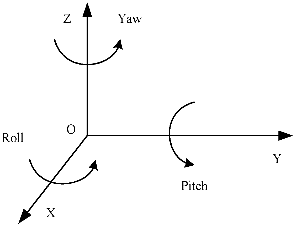
As Figure 1 shows, the attitude angles of an IMU are the three angles between the coordinate system and the ground inertial coordinate system, which can be represented by the roll angle, pitch angle, and yaw angle. The roll angle can be obtained by the rotation around the X-axis, the pitch angle can be obtained by the rotation around the Y-axis, and the yaw angle can be obtained by the rotation around the Z-axis [19].

The magnetic measurement value of a certain point on Earth is $h=\left[h_x^b,h_y^b,h_z^b\right]$, which, respectively, represents the components of the measured value of the three-axis dynamometer along each axis, the magnetic field vector under the geomagnetism, and the projection of the magnetic field vector under the magnetometer coordinate system. When it is parallel to the geomagnetic plane, the angle between the magnetometer and the geomagnetic north pole can be calculated according to Equation (1) [20].

$$\varphi =\arctan (\frac{h_y^b}{h_x^b})$$

(1)

In an IMU, $M_x^m,M_y^m,M_z^m$ represent axis components of geomagnetic intensity measured by magnetometer in the magnetometer coordinate system. $M_x^b,M_y^b,M_z^b$ represent the corrected values of each axis of geomagnetic field intensity in the magnetometer coordinate system. The slant angle of the magnetometer can be corrected by the accelerometer as shown in Equation (2).

$$\left[\begin{array}{l}{M}_x^b\\ M_y^b\\ M_z^b\end{array}\right]=\left[\begin{array}{ccc}\cos \theta & 0& \sin \theta \\ \sin \gamma \sin \theta & \cos \gamma & -\sin \gamma \cos \theta \\ -\cos \gamma \sin \theta & \sin \gamma & \cos \gamma \cos \theta \end{array}\right]\left[\begin{array}{l}{M}_x^m\\ M_y^m\\ M_z^m\end{array}\right]$$

(2)

The yaw angle of the moving object carrying the IMU can be obtained according to Equation (3):

$$\varphi =\arctan (\frac{M_y^b}{M_x^b})$$

(3)

The pitch angle and roll angle are calculated according to the components of gravity on each axis of the moving object measured by the accelerometer.

$$\left[\begin{array}{l}{A}_x^b\\ A_y^b\\ A_z^b\end{array}\right]=\left[\begin{array}{ccc}\cos \theta \cos \varphi & \cos \theta \sin \varphi & -\sin \theta \\ \sin \gamma \sin \theta \cos \varphi -\cos \gamma \sin \varphi & \sin \gamma \sin \theta \sin \varphi +\cos \gamma \cos \varphi & \sin \gamma \cos \theta \\ \cos \gamma \sin \theta \cos \varphi +\sin \gamma \sin \varphi & \cos \gamma \sin \theta \sin \varphi -\sin \gamma \cos \varphi & \cos \gamma \cos \theta \end{array}\right]\left[\begin{array}{l}0\\ 0\\ 1\end{array}\right]$$

(4)

where $A_x^b,A_y^b,A_z^b$ represent the gravity components measured by the accelerometer in each axis direction, and the vector represents the gravity field component measured by the accelerometer in each axis in the geographic coordinate system. In this study, θ represents the pitch angle, and γ represents the roll angle. θ can be obtained using the above equation and the expression seen in Equations (5) and (6).

$$\theta =\arcsin (-A_x^a)$$

(5)

$$\gamma =\arcsin (\frac{A_y^a}{\cos \theta })$$

(6)

Based on the equations above, the position and pose information of the moving object where an IMU is installed can be obtained.

$$\left[\varphi , \theta , \gamma \right]=[\arctan (\frac{M_y^b}{M_x^b}),\arcsin (-A_x^a),\arcsin (\frac{A_y^a}{\cos \theta })]$$

(7)

3.2. Extended Kalman Filter

Extended Kalman filter (EKF) technology is utilized to make an optimal estimation of the state of a nonlinear system. A linear time-varying system can be used to describe a nonlinear system within each sampling interval, and then the linear time-varying system can use the Kalman filter (KF). The corresponding processes are as follows [21].

3.2.1. Definition of State Space

The general form of the mathematical model of a nonlinear discrete system can be expressed in Equation (8).

$$\left\{\begin{array}{l}{x}_k=f(x_{k-1},u_{k-1},w_{k-1})\\ y_k=h(x_k,v_k)\end{array}\right.$$

(8)

where $x_k$ is the state vector of the system at moment k, $u_{k-1}$ is the input vector of the system at moment k − 1, $w_{k-1}$ is the stationary noise sequence of the process of the system at moment k − 1, $f\left(\right)$ is the state transition function of the system and nonlinear (or linear) function of the state $x_{k-1}$, $y_k$ is the measurement vector of the system at moment k, $v_k$ is the noise sequence of the system at moment k, and w and v satisfy normal distribution.

3.2.2. Linearization

We linearized the system mathematically at the point $\left({\widehat{x}}_k,{\widehat{x}}_{k-1}\right)$ as

$$\left\{\begin{array}{l}f(x_{k-1},u_{k-1},w_{k-1})\approx f({\widehat{x}}_{k-1},u_k,0)+\frac{\partial f}{\partial x_{k-1}}(x_{k-1}-{\widehat{x}}_{k-1})+\frac{\partial f}{\partial w_k}{w}_k\\ h(x_k,v_k)=h({\widehat{x}}_k,0)+\frac{\partial f}{\partial v_k}{v}_k\end{array}\right.$$

(9)

Under the linear system approximation, both the noise terms and the states are regarded as Gaussian distributions. Therefore, states can be described by estimating their mean and covariance matrices.

3.2.3. Kalman Gain

In this process, the transition matrix, observation matrix, and optimal state value of the system can be described as

$$P_k^{-}=F_{k-1}{P}_{k-1}{F}^T{}_{k-1}+Q^{\prime }{}_k$$

(10)

$$K_k=\frac{P_k^{-}{H}_k^T}{H_{\mathrm{k}}{P}_k^{-}{H}_k^T+R_k^{\prime }}$$

(11)

$${\widehat{x}}_k={\widehat{x}}_k^{-}+K_k(y_k-h({\widehat{x}}_k,0))$$

(12)

$$P_k=(I-K_k{h}_{\mathrm{k}})P_k^{-}$$

(13)

where

$$F_{k-1}={\left.\frac{\partial f}{\partial x_{k-1}}\right|}_{{\widehat{x}}_{k-1}},H_k^T={\left.\frac{\partial f}{\partial x_k}\right|}_{{\widehat{x}}_k}$$

(14)

$$Q^{\prime }{}_k=wQ{w}^T,R_k^{\prime }=vR{v}^T$$

(15)

4. Improved Tight Combination Model

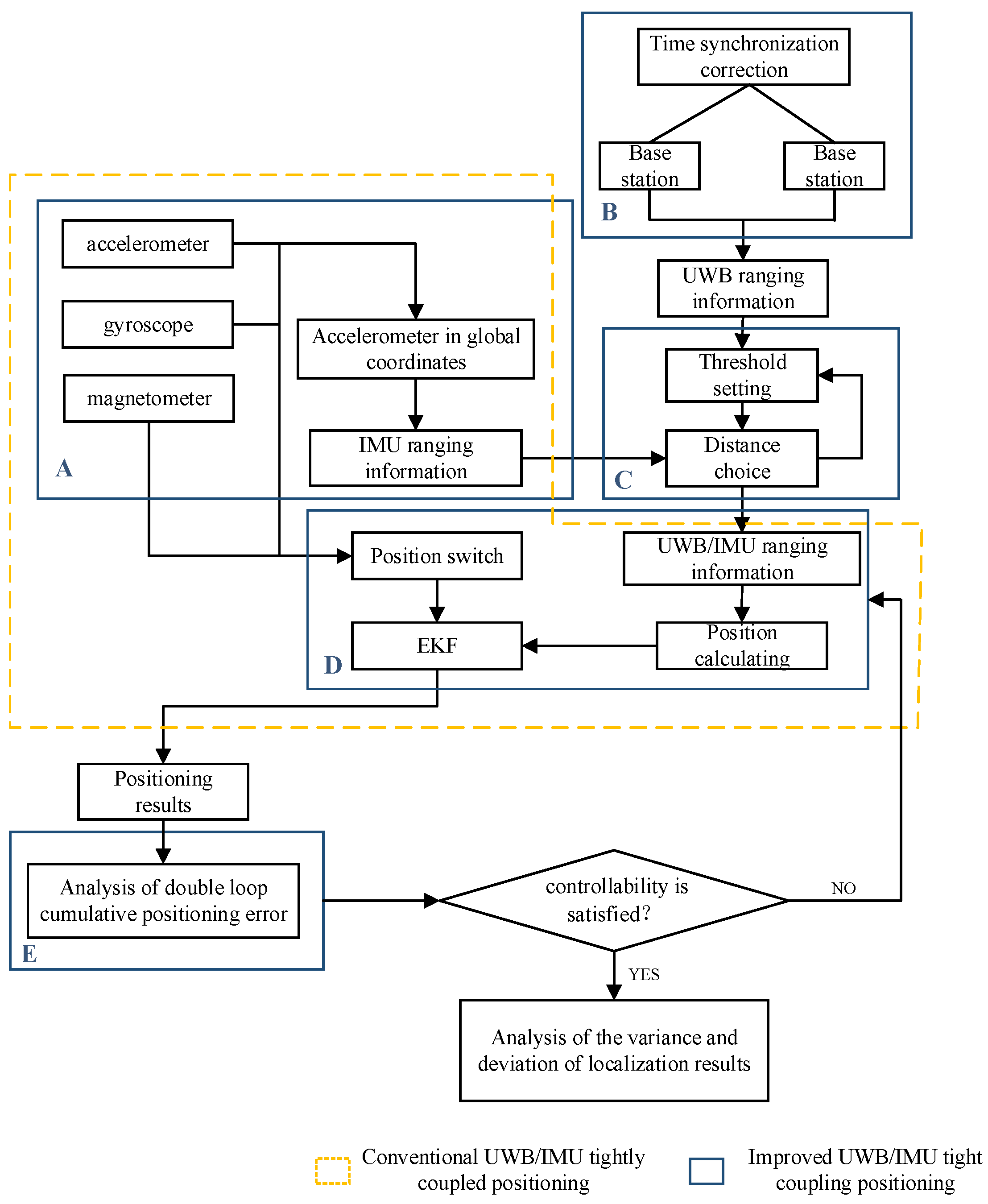
To prevent positioning failure due to uncontrollable and cumulative errors from IMUs, we improved the UWB/IMU combination model with new modules for fixing time desynchronization, optimizing the threshold setting for UWB ranging, data fusion in NLOS, and double-loop error self-correction. As Figure 2 shows, first, the distance information obtained by the second integral of the IMU accelerometer was converted to the global coordinate. According to the triangular three-side principle, the UWB ranging information was filtered by removing the positioning error caused by NLOS, and the optimized UWB ranging information was converted to the location information as the UWB output and EKF input.

In Figure 2, this improved model can be divided into four parts: (1) doubling the IMU acceleration integration by time to obtain distance information, as shown in module A; (2) UWB time non-synchronous correction to obtain range information, as shown in module B; (3) distance threshold setting and UWB ranging information optimization, as shown in module C; (4) improvement of the UWB/IMU tight combination positioning model establishment, as shown in module D.

To make the cumulative errors from IMUs controllable, the positioning results are input into the module E, i.e., the module of analysis of the dynamic double-loop cumulative positioning error. Then, the analysis result can be judged according to whether the controllability is satisfied. If the result is “yes,” then the localization results will be analyzed for the performances of variance and deviation. Otherwise, if the result is “no”, the current positioning results will be ignored, and the workflow returns back to module D for new position calculation until the positioning system controllability is satisfied.

4.1. IMU Location Calculation

The measured values of IMU are w and a. When calculating the position, velocity, and quaternion, the IMU measurements need to be integrated by time. From moment i = 0 to k, the measured value of IMU was integrated, and the expression of PVQ obtained is shown in Equation (16), where g is gravity acceleration of one point on earth, and g = 9.8 m/s².

$$\begin{array}{l}{p}_{k+1}=p_k+T_{i->j}{v}_k+{\displaystyle \underset{t\in [i,j]}{\iint }(a_k-g)}d{t}^2\\ v_{k+1}=v_k+{\displaystyle \underset{t\in [i,j]}{\int }(a_k-g)}dt\end{array}$$

(16)

4.2. Time Synchronization Correction

In fact, the CPU clocks of the positioning base stations are different. Even if the clocks can be corrected periodically, the synchronization error and the positioning error can hardly be completely eliminated.

In general, a time offset of 1 ns with an optical speed can cause a 30 cm position error theoretically. To minimize the positioning error, the clock offsets of all on-field base stations can be corrected before the base station ranging. Therefore, although the difference between the non-synchronized clock only exists at the picosecond level, with light speed, it can still cause a few meters’ error in the ranging result. Among them, the offset between the crystal clock and the system global clock, as well as the antenna delay, are the two remarkable factors leading to the UWB clock offset. The overall clock model is shown in Equation (17) [22]:

$$t^M={\alpha }_f^{M}t+{\beta }_t^M\pm {\tau }^M$$

(17)

where ${\alpha }_f^M$ is the normalized process based on the system reference clock, and the value is approximately 1; ${\beta }_t^M$ is the clock offset based on the system reference clock; and ${\tau }^M$ is the antenna delay error.

To reduce the errors above, a counter can be used to synchronize the timestamp from a slave base station to the master base station. When calculating the time synchronization for the kth moment, the clock drift (offset) rate between time k and k − 1 can be calculated. For wireless clock synchronization k, its clock drift rate is

$$y_k=\frac{T_{B_k}-T_{B{1}_{k-1}}}{T_{A_k}-T_{A_{k-1}}}$$

(18)

When the timestamp signal is received between the wireless clock synchronization moments k and k + 1, the value of the timestamp of the slave base station is $C_k$. At this moment, the timestamp of the slave base station receiving the label signal is synchronized to the timestamp of the master base station, and the synchronization time is

$$T=T_{A_k}+\frac{C_k-T_{B_k}}{y_k}+T_{AB}$$

(19)

where $T_{AB}$ is the flight time between the base master station A and slave station B, which is determined by the distance between these two base stations.

4.3. Distance Threshold Setting

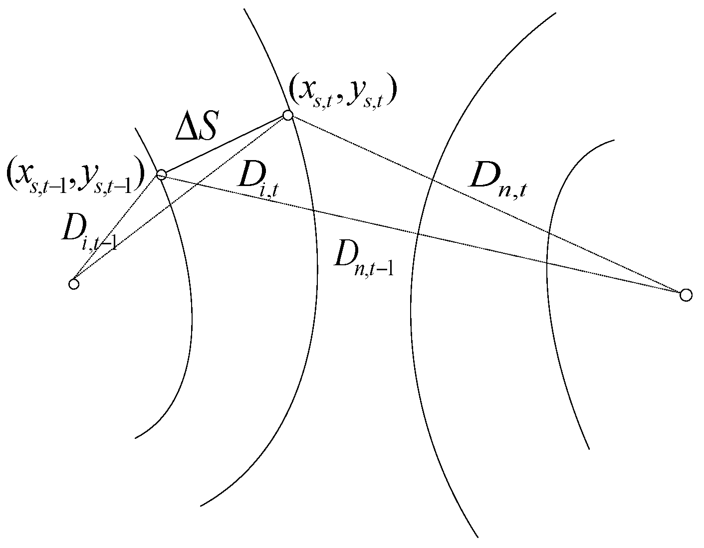
The location information can be optimized by setting the threshold to eliminate the poor location data of UWB under NLOS. The TDOA positioning method and triangle three-side theorem [23] were used to set the threshold, as shown in Figure 3.

The equation group corresponding to Figure 3 can be obtained as

(1) In triangle ABC,

$$\begin{array}{l}\Delta S+D_{i,t-1}-D_{i,t}>0\\ \Delta S+D_{i,t}-D_{i,t-1}>0\\ D_{i,t-1}+D_{i,t}-\Delta S>0\end{array}$$

(20)

(2) In triangle ABD,

$$\begin{array}{l}\Delta S+D_{n,t-1}-D_{n,t}>0\\ \Delta S+D_{n,t}-D_{n,t-1}>0\\ D_{n,t-1}+D_{n,t}-\Delta S>0\end{array}$$

(21)

The combination results are shown in Equation (22):

$$\begin{array}{l}2\Delta S+D_{i,t}-D_{n,t}+D_{n,t-1}-D_{i,t-1}=2\Delta S+\Delta d_{in,t}-\Delta d_{in,t-1}>0\\ 2\Delta S+D_{n,t}-D_{i,t}+D_{i,t-1}-D_{n,t-1}=2\Delta S+\Delta d_{in,t-1}-\Delta d_{in,t}>0\end{array}$$

(22)

From the state vector, the relative distance $∆S$ between the current position and the starting position can be obtained by taking the measured value of the accelerometer for the second integral with time, and the distance threshold can be obtained as

$$2\Delta S-\left|\right|\Delta d_{in,t-1}-\Delta d_{in,t}\left|\right|>0$$

(23)

Because an IMU has the advantage of short time and high-precision positioning, this threshold above can be used to filter the UWB poor data that are bigger than the distance threshold.

4.4. Design of Extended Kalman Filter

The state equation and measurement equation of the system based on the improved UWB/IMU tight combination positioning model were derived based on the extended Kalman filter. In this study, the position, velocity, and acceleration of an IMU were selected as state variables, and the ranging information of UWB and the angle information of IMU were selected as observation values.

4.4.1. System State Equation

The state equation of the tight combination in this improved UWB/IMU is

$$X(k+1)=FX(k)+\Gamma w(k)$$

(24)

where $X(k)={[{(p_k^{\mathrm{n}})}^T,(v_k^{\mathrm{n}}),(a_k^{\mathrm{n}})]}^T$ is the state vector of the carrier at time k, w(k) is the process noise, $w(k)~N(0,Q)$,$Q=\left[\begin{array}{cc}{\sigma }_{a,x}& 0\\ 0& {\sigma }_{a,y}\end{array}\right]$,$F=\left[\begin{array}{ccc}{I}_2& T{I}_2& T^2/2I_2\\ O_2& I_2& T{I}_2\\ O_2& O_2& I_2\end{array}\right]$ is the state transition matrix, $\Gamma =\left[\begin{array}{c}{T}^3/6I_2\\ T^2/2I_2\\ T{I}_2\end{array}\right]$ is the noise drive matrix, T is the length of time from i = 0 to k, and $I_2$ is the unit matrix of 2 × 2.

4.4.2. Measurement Equation

The measurement equation of the tight combination based on the improved UWB/IMU is shown in Equations (25) and (26).

$$Y(k)=HX(k)+Dv(k)$$

(25)

$$Y(k)=\left[\begin{array}{c}△d_{1,k}\\ △d_{2,k}\\ ⋮\\ △d_{n,k}\end{array}\right]$$

(26)

The corresponding measurement information is the ranging difference between IMU and UWB.

$$H=\left[\begin{array}{cccc}\frac{\partial d_{{}_{1,k}}^{{}^{imu}}}{\partial p_{{}_x}^n}& \frac{\partial d_{{}_{1,k}}^{{}^{imu}}}{\partial p_y^n}& O_2& O_2\\ \frac{\partial d_{{}_{2,k}}^{{}^{imu}}}{\partial p_{{}_x}^n}& \frac{\partial d_{{}_{2,k}}^{{}^{imu}}}{\partial p_y^n}& O_2& O_2\\ ⋮& ⋮& ⋮& ⋮\\ \frac{\partial d_{{}_{n,k}}^{{}^{imu}}}{\partial p_{{}_x}^n}& \frac{\partial d_{{}_{n,k}}^{{}^{imu}}}{\partial p_{{}_x}^n}& O_2& O_2\end{array}\right]$$

(27)

where H is measurement matrix; n is the amount of data measured by IMU after passing the threshold; and v(k) is the measurement noise, with $v(k)~N(0,R)$.

Thereby, the extended Kalman gain can be determined based on Equations (10)–(13), including the transition matrix, observation matrix, and optimal state value of the system.

4.5. Convergence Analysis of Combination Error

4.5.1. Accumulative Error Analysis of IMU after Twice Integral

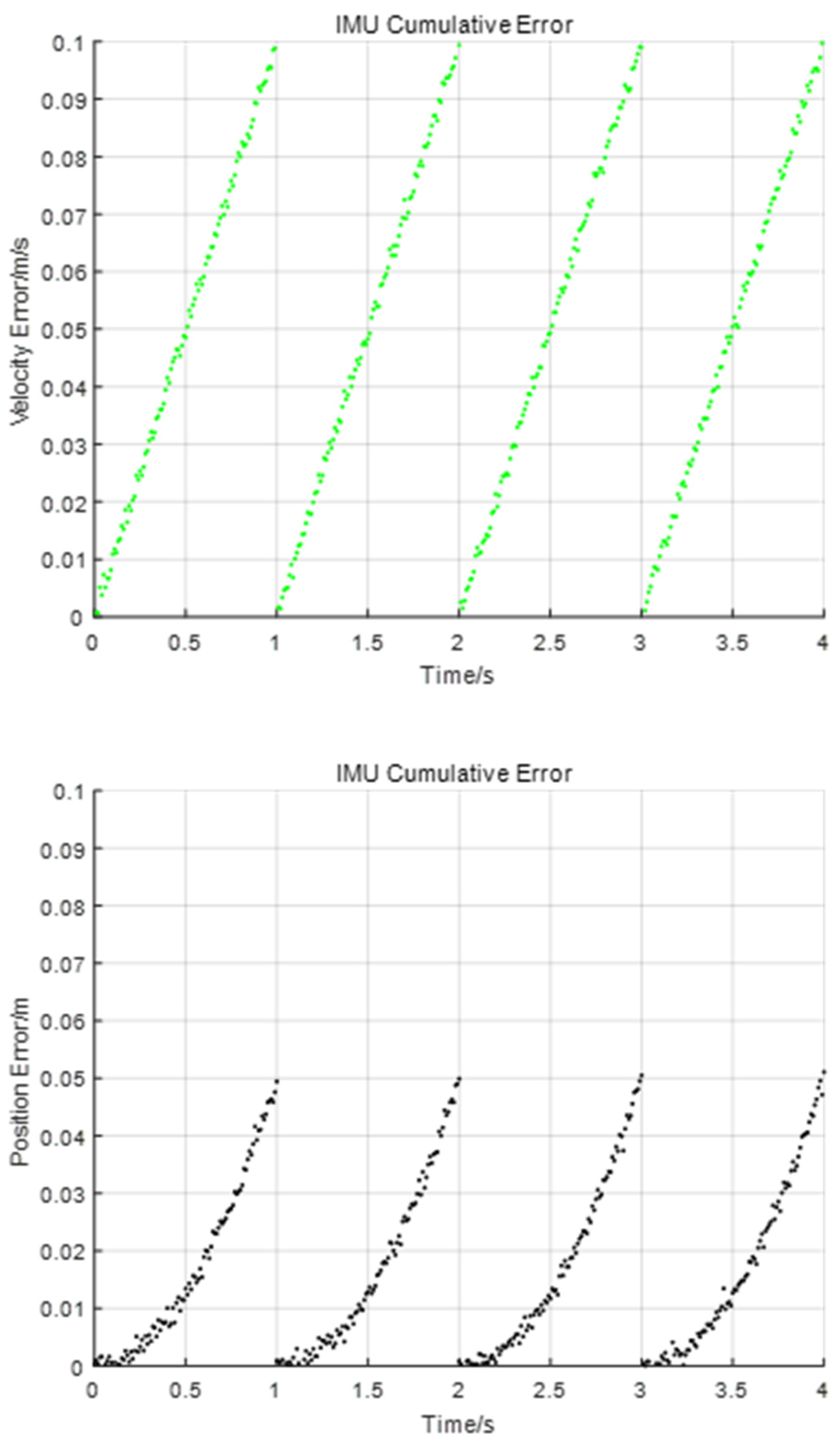
In theory, the output value of IMU should be 0 when it is idle. However, as Equation (26) shows, due to the offset b of all three axes and the need to integrate the acceleration value when calculating the motion speed and relative position, the offset b and Gaussian white noise n will participate in the integration calculations by time. Subsequently, the result error of velocity and displacement calculation will become larger with the increase in time.

When the offset b was set to 0.01, the Gaussian white noise was 80, and the error was eliminated every second, we obtained the cumulative error of IMU speed and position within 4 s, as shown in the Figure 4.

$$v_{err}=b^{a}t,p_{err}=\frac{1}{2}{b}^a{t}^2$$

(28)

4.5.2. Cumulative Error Analysis of EKF-Based Positive Feedback

Regarding the module of EKF, the positioning state error $e_t=x_t-\widehat{x_t}$. According to EFK, linearizing f at $\widehat{x_t}$, that is, Taylor expansion, is used to expand the error to obtain the error linear transfer equation [24].

$$\begin{array}{ll}{\dot{e}}_t& ={\dot{x}}_t-{\dot{\widehat{x}}}_t\\ & =f(x_t,u_t)+n_t-{\dot{\widehat{x}}}_t\\ & =f({\widehat{x}}_t,u_t)+F_{{\widehat{x}}_t,u_t}(x_t-{\widehat{x}}_t)+n_t-{\dot{\widehat{x}}}_t\\ & =F_{{\widehat{x}}_t,u_t}(x_t-{\widehat{x}}_t)+n_t\\ & =F_{{\widehat{x}}_t,u_t}{e}_t+n_t\end{array}$$

(29)

It can be found from Equation (29) that, when noise is applied, the state estimator cannot be predicted, which leads to the failure of system convergence. When the estimate and the true value of the difference is large, the system matrix F will have larger deviation. If we use F to transmit the error, then the error transfer system will form positive feedback, which will eventually cause the filter to diverge.

Meanwhile, the error between the actual measured value and the estimated observation is $Z_t=y_t-\widehat{y_t}$. With same principle, Taylor expansion is used again for hat $\widehat{x_t}$, and the linear transfer equation of error is shown in Equation (28) [25].

$$\begin{array}{ll}{z}_t& =y_t-{\widehat{y}}_t\\ & =h(x_t)+s_t-{\widehat{y}}_t\\ & =h({\widehat{x}}_t)+H_{{\widehat{x}}_t}(x_t-{\widehat{x}}_t)+s_t-{\widehat{y}}_t\\ & =H_{{\widehat{x}}_t}{e}_t+s_t\end{array}$$

(30)

It can be found from the equation that the relationship between the state error and the observation error is approximate. Therefore, when there is a large gap between the observed value and the estimated value, the system matrix H at this time will also have a large deviation, and the error will be further amplified after the error continues to be transmitted by H.

4.5.3. Dynamics Model of Double-Loop Cumulative Error

In this study, an IMU was introduced to reduce the positioning error caused by NLOS interferences. However, since the second integrations by the time of IMU acceleration leads to an accumulated error, the UWB error propagation dynamics model and IMU position cumulative error in this study were used to establish the double-loop cumulative error dynamics model (DCEM), as shown in Equations (31) and (32).

$$e_{DEPM}={\omega }_1{E}_1+{\omega }_2{E}_2$$

(31)

$$e={\omega }_{UWB}{e}_{DEPM}+{\omega }_{IMU}{e}_{IMU}$$

(32)

In the ith filtering fusion, the state vector at k − 1 moment is used to derive the estimate of the prior error state at k moment.

$$e_k^{-}=F_1{X}_{k-1}^e$$

(33)

where $F_{\mathrm{2,3}}$ is the first-order expression of each part of the state transition matrix F. In this case, the error state vector at moment k can be kinked with the error state vector at moment k − 1.

In the discrete positioning system, the error is constantly iterated in the system state equation. When the iteration reaches the kth moment, the IMU error is eliminated back to zero, and the j at the next moment is set as j + 1 and i as i + 1. In this way, the convergence of IMU cumulative error is effectively controlled.

4.5.4. Controllability Analysis of the Sensor-Fusion Error Transmission System

According to the modern control theory, a system is completely controllable when there is an unconstrained input signal u(t) that can make the system change from any initial state X₀ to another expected state X.

For the state variables system:

$$\dot{x}=Ax+Bu$$

(34)

Considering whether the algebraic conditions of Equation (34) are valid, it can be determined whether the system is completely controllable, where A is the system matrix of n × n dimension, B is the control matrix of n × m dimension, and m is the number of input signals.

$$rank\left[\begin{array}{ccccc}B& AB& A^{2}B& \cdots & A^{n-1}B\end{array}\right]=n$$

(35)

For an IMU, the noise disturbance is equivalent to the unconstrained input signal, and the position, velocity, and acceleration of the carrier are measured at each moment as state variables. According to the definition of the fully controllable system, it can be found that the IMU cannot be fully controllable under the influence of the integration calculation error. However, in the double-loop cumulative error model, the error controllability can be introduced because the error state vector at moment k is correlated with the error state quantity at moment k − 1 during the ith filter fusion, as demonstrated in the simulation experiments in Section 5.

5. Simulation Experiments

In indoor space, the positioning accuracy and precision of UWB are often affected by the surroundings of a positioning object. To validate the improved UWB/IMU tight combination model proposed in this study, the MATALB R2020a simulation tool was used to calculate the difference between the distance obtained by the secondary time-integration of the IMU accelerometer and UWB ranging. Then, the tool eliminated the results larger than the distance threshold to finally obtain more accurate position according to the filtered UWB distance results.

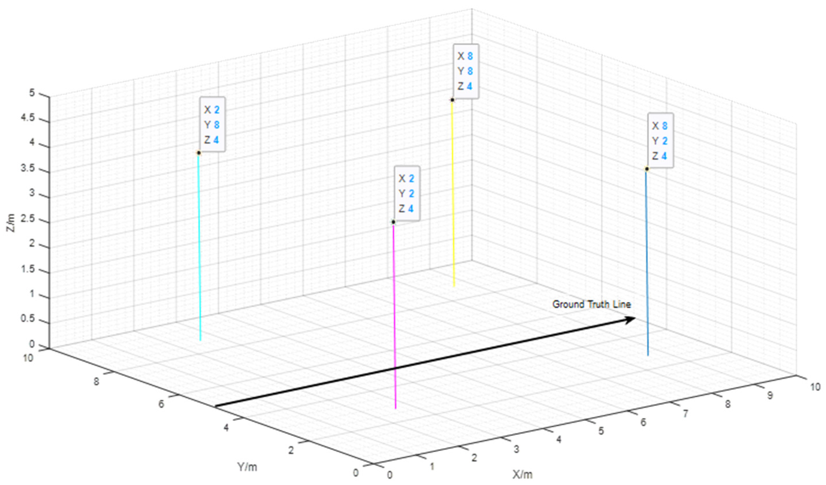
The simulation experiment was set in a space of 10 m × 10 m × 5 m (i.e., length × width × height). We used the UWB hardware (UWB tag, base station) and software (measurement tool) supplied by Woxu Wireless Company [26] to validate the improved UWB/IMU positioning. We marked the ground truth line with a black belt on the ground as shown in Figure 5. The red and blue circles represent the location of the base stations, which were (2, 2, 4) as an endpoint of a pink line, (2, 8, 4) as an endpoint of a cyan line, (8, 2, 4) as an endpoint of a blue line, and (8, 8, 4) as an endpoint of a yellow line, and the red asterisk point represents the origin coordinate (0, 0).

We used the MATLAB 2019a robotics system toolbox to set the position and attitude of the trajectory passing point to automatically generate a smooth motion trajectory. The target motion state included linear motion, curve motion, acceleration, deceleration, and uniform motion. In this experiment, the linear moving object was analyzed, and the motion speed was controlled within 4 m/s.

5.1. Motion Trajectory Analysis

In the experimental scenarios above, we set the abscissa x to increase linearly within the range of [0, 10], and the straight-line y was always maintained at 5 as the reference track, as shown in Figure 6. The obstacles in the experimental simulation were regarded as Gaussian white noise, set to 40, and added to the vector signal X. Considering the atmospheric interference at this time, Gaussian white noise was set to 60 and added to the vector signal X.

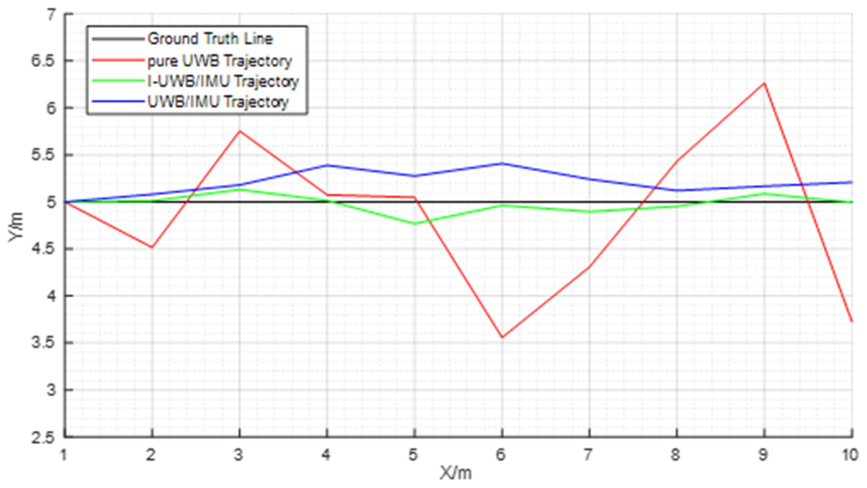
Furthermore, the motion position had a certain deviation. Therefore, the following three kinds of data were analyzed: (1) IMU acceleration, velocity, and position data optimized by EKF; (2) for the collected UWB and IMU data, the position data obtained using the tight combination of the improved UWB/IMU were compared with the pure UWB position data; (3) the positioning error data, including the maximum deviation, minimum deviation, and standard deviation, as well as the analysis of the error controllability of the system. The following observations can be seen from Figure 7 and

Table 1. Deviations in I-UWB/IMU, UWB/IMU, and pure UWB positioning.

Method/Model	Maximum Deviation (m)	Standard Deviation (m)
Pure UWB	1.444	0.8567
UWB/IMU	0.408	0.1283
I-UWB/IMU	0.232	0.0998

:

• The UWB location had the largest standard deviation, and the improved fusion location had the smallest.
• The improved UWB/IMU fusion model could eliminate the cumulative error of IMU at the same period and ensure the accuracy of positioning system.
• The improved UWB/IMU fusion model made the error meet the controllability requirement of the system better.

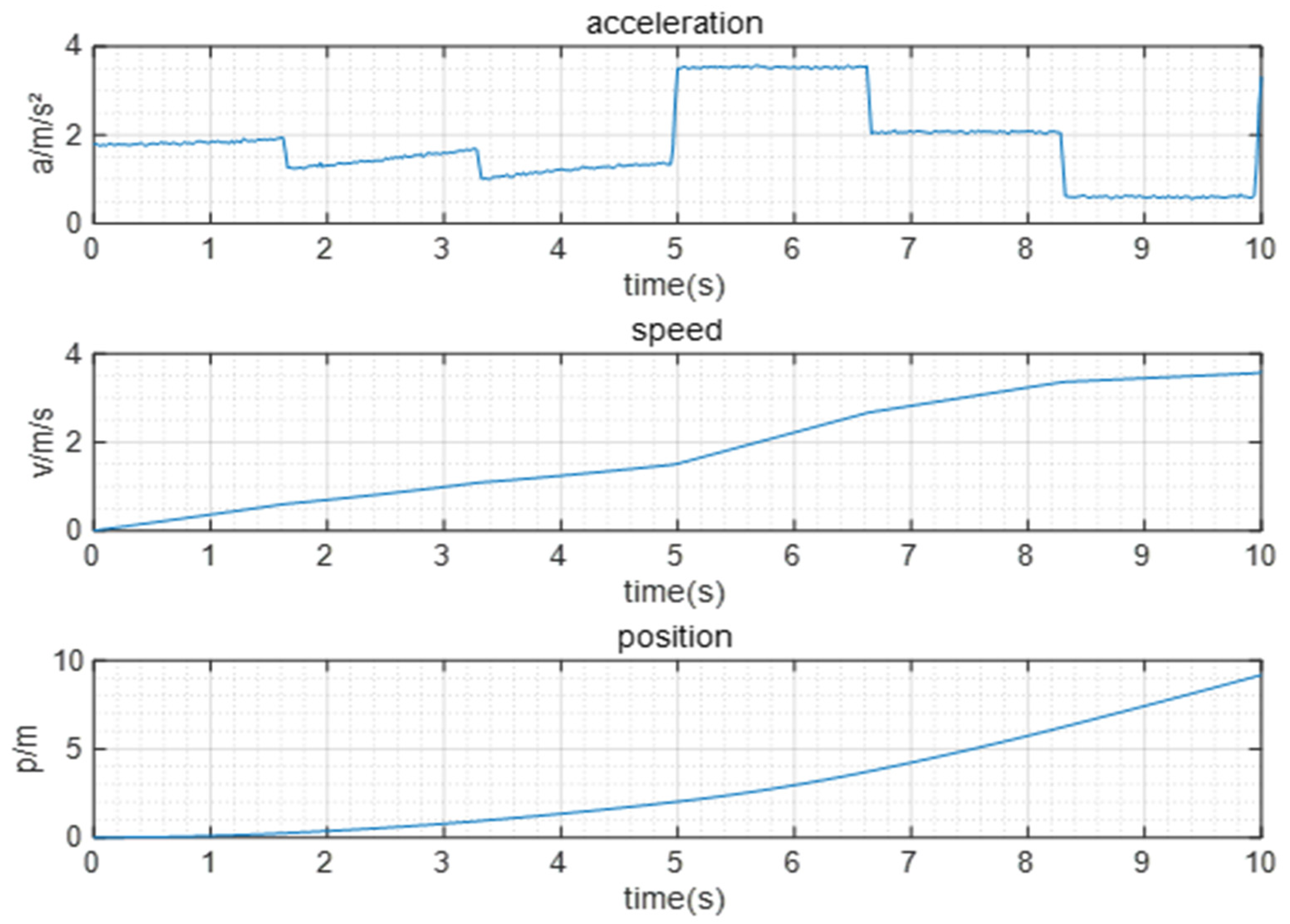
5.2. Acceleration KF-Based Optimization Model

The acceleration value of IMU was integrated and converted to obtain the velocity and position, as shown in Figure 6. Then, the obtained data were filtered based on EKF technology.

IMU measured the initial position of the carrier as the origin of the coordinates. Therefore, it can be seen from Figure 6 that as the distance of the X-axis changed from 0, the acceleration signal and speed signal appeared smoother and more stable after filtering, and the speed kept changing within 4 m/s.

5.3. Analysis for Improved UWB/IMU Tight Combination Positioning Model

To verify the effectiveness of the algorithm, this study compared the pure UWB (i.e., only ranging UWB) positioning system with the improved model based on the UWB/IMU tight combination and EKF filter positioning system. The pure UWB positioning system only uses the UWB ranging information for position calculation. The position information output is unstable and has a large position offset, with the maximum error reaching 2 m.

The improved model could control the error within 0.3 m during 75% of the experiment and converge the positioning trajectory to the real value faster, which shows that the improvement based on the combined positioning model of EKF could effectively track the position of the target. The IMU could remove the data that cannot be identified by the filter in the traditional model in advance, and the remaining data optimize the UWB positioning results. This greatly eliminates the impact of NLOS interference on pure UWB systems [27,28].

The comparison chart of trajectory and positioning results is shown in Figure 7. The chart shows that along the Y-axis direction, the absolute value of the maximum deviation of the pure UWB reached 1.444 m, the maximum deviation of the conventional UWB/IMU reached 0.408 m, and the absolute value of the maximum deviation of the UWB/IMU was only 0.232 m.

In Table 1, error reduced by 1 − (0.232/1.444) = 83.93%, 1 − (0.232/0.408) = 43.14%, and standard deviation reduced by 1 − (0.0998/0.8567) =88.35%, 1 − (0.0998/0.1283) = 22.21%, so the improved UWB/IMU tight combination positioning results (as the greed line) were far better than the pure UWB (as the red color line) shown in Figure 7.

The I-UWB/IMU was the improved UWB/IMU tight combination positioning model proposed in this paper, and UWB/IMU is the conventional UWB/IMU tight combination positioning model.

In this experiment, the time interval was 1, i = 1, j = 0, k = 0.02; the system matrix was F; and the control matrix was $\Gamma$.

$$F=\left[\begin{array}{ccc}{I}_2& I_2& 1/2I_2\\ O_2& I_2& I_2\\ O_2& O_2& I_2\end{array}\right],\Gamma =\left[\begin{array}{c}1/6I_2\\ 1/2I_2\\ I_2\end{array}\right]$$

(36)

According to Equations (34) and (35), the rank of the matrix F was 3, and the system did not satisfy the complete controllability. In the case of the double-loop accumulated error in this study, the F and $\Gamma$, as shown in Equation (37), are as follows:

$$F=\left[\begin{array}{ccc}I& I& 1/2I\\ O& I& I\\ O& O& I\end{array}\right],\Gamma =\left[\begin{array}{c}1/6I\\ 1/2I\\ I\end{array}\right]$$

(37)

According to Equation (35), the controllable matrix of the system could be calculated as

$$P=\left[\begin{array}{ccc}0.1667& 1.1667& 3.1667\\ 0.5000& 1.5000& 2.5000\\ 1.0000& 1.0000& 1.0000\end{array}\right]$$

(38)

The rank of the matrix P was 3, and the system was completely controllable, proving that the error of the system was controllable with the elimination approach of the double-loop accumulated error.

5.4. Discussion

In the experimental result analysis part, the improved UWB/IMU tight combination model was numerically validated. The experimental results showed that the improved UWB/IMU tight combination model remarkably enhanced the positioning accuracy with a maximum deviation of 0.232 m (reduced by 83.93% compared to a pure UWB model and 43.14% compared to the conventional UWB/IMU model) and standard deviation of 0.09981 m (reduced by 88.35% compared to a pure UWB model and 22.21% compared to the conventional UWB-IMU model).

In the application of the real-world scene, positioning accuracy will be affected by obstacles or moving pedestrians in most real-world scenes. It is necessary to consider the matching problem of the IMU cumulative error elimination step and the UWB elimination error step in future research, and it is also important to modify the parameters in the extended Kalman filter to increase the generalization ability of the dynamic double-loop cumulative error estimation model.

6. Conclusions

This study first analyzed the principle of IMU positioning and EKF technology. Then, based on the traditional UWB/IMU tight combination methods, an improved tight combination positioning model was proposed, and three new modules were proposed. The distance information obtained by the second time integral of the IMU accelerometer was used to optimize the UWB ranging information and convert the location information as UWB output and EKF input.

The combination model reduced the positioning deviation at each moment and the overall positioning standard deviation. Furthermore, based on the proposed dual-loop cumulative error model and modern control theory, it was proven that the error of the proposed model satisfied the controllability. In this study, an IMU was used as an auxiliary sensor to optimize the ranging data of the UWB, but the positioning accuracy still mainly depended on the ranging accuracy of the UWB.

In the future, new research can introduce visual positioning technologies to monitor environmental occlusions and other conditions in real time, utilize map information created by computer vision to improve data fusion technology, and perform the real-time correction of ranging information to achieve further high-precision positioning in complex indoor environments.

References

- Filippoupolitis, A.; Oliff, W.; Loukas, G. Bluetooth Low Energy Based Occupancy Detection for Emergency Management. In Proceedings of the International Conference on Ubiquitous Computing and Communications, Granada, Spain, 14–16 December 2016. [Google Scholar]
- Tekler, Z.D.; Low, R.; Yuen, C.; Blessing, L. Plug-Mate: An IoT-based occupancy-driven plug load management system in smart buildings. Build. Environ. 2022, 223, 109472. [Google Scholar] [CrossRef]
- Tekler, Z.D.; Low, R.; Gunay, B.; Andersen, R.K.; Blessing, L. A Scalable Bluetooth Low Energy Approach to Identify Occupancy Patterns and Profiles in Office Spaces. Build. Environ. 2020, 171, 106681. [Google Scholar] [CrossRef]
- Yassin, A.; Nasser, Y.; Awad, M.; Al-Dubai, A.; Liu, R.; Yuen, C.; Raulefs, R.; Aboutanios, E. Recent Advances in Indoor Localization: A Survey on Theoretical Approaches and Applications. IEEE Commun. Surv. Tutor. 2016, 19, 1327–1346. [Google Scholar] [CrossRef]
- Li, H. Research on Indoor Positioning Method Based on Multi-Sensor Combination. Ph.D. Thesis, Nanchang University, Nanchang, China, 2020. Volume 19, pp. 1327–1346. (In Chinese). [Google Scholar]
- Tian, Q.; Wang, K.I.; Salcic, Z. A Low-Cost INS and UWB Fusion Pedestrian Tracking System. Sens. J. 2019, 19, 3733–3740. [Google Scholar] [CrossRef]
- Liu, F.; Li, X.; Wang, J.; Zhang, J. An Adaptive UWB/MEMS-IMU Complementary Kalman Filter for Indoor Location in NLOS Environment. Remote Sens. 2019, 11, 2628. [Google Scholar] [CrossRef]
- Yue, X.; Jiang, Z.; Guo, P.; Li, H.; Liu, X.; Li, M.; Liu, F. Research on Fusion and Location Method of Indoor Targeted Spraying Robots Based on UWB\IMU. In Proceedings of the 2022 IEEE 6th Information Technology and Mechatronics Engineering Conference (ITOEC), Chongqing, China, 4–6 March 2022; Volume 2022, pp. 1487–1492. [Google Scholar]
- Shi, Y.; Zhang, Y.; Li, Z.; Yuan, S.; Zhu, S. IMU/UWB Fusion Method Using a Complementary Filter and a Kalman Filter for Hybrid Upper Limb Motion Estimation. Sensors 2023, 23, 6700. [Google Scholar] [CrossRef]
- Delamare, M.; Boutteau, R.; Savatier, X.; Iriart, N. Evaluation of an UWB localization system in static and dynamic. In Proceedings of the Internation Conference on Indoor Positioning and Indoor Navigation (IPIN), Pisa, Italy, 30 September–3 October 2019. [Google Scholar]
- Nguyen, T.H.; Nguyen, T.M.; Xie, L. Range-Focused Fusion of Camera-IMU-UWB for Accurate and Drift-Reduced Localization. Robot. Autom. Lett. 2021, 6, 1678–1685. [Google Scholar] [CrossRef]
- Khan, O.; Bergelt, R.; Hardt, W. On-field mounting position estimation of a lidar sensor. In Remote Sensing Technologies and Applications in Urban Environments II, Proceedings of the SPIE Remote Sensing 2017, Warsaw, Poland, 11–14 September 2017; SPIE: Bellingham, WA, USA, 2017; Volume 10431, pp. 191–197. [Google Scholar]
- Deng, T.; Bazin, J.C.; Martin, T.; Kuster, C.; Cai, J.; Popa, T.; Gross, M. Registration of multiple RGBD cameras via local rigid transformation. In Proceedings of the International Conference on Multimedia and Expo (ICME), Chengdu, China, 14–18 July 2014. [Google Scholar]
- Koppanyi, Z.; Navratil, V.; Xu, H.; Toth, C.K.; Grejner-Brzezinska, D. Using Adaptive Motion Constraints to Support UWB/IMU Based Navigation. J. Inst. Navig. 2018, 65, 247–261. [Google Scholar] [CrossRef]
- Basar, T. A New Approach to Linear Filtering and Prediction Problems. In Control Theory: Twenty-Five Seminal Papers (1932–1981); Wiley-IEEE Press: Hoboken, NJ, USA, 2001; pp. 167–179. [Google Scholar]
- Li, Q.; Li, R.; Ji, K.; Dai, W. Kalman Filter and Its Application. In Proceedings of the 2015 8th International Conference on Intelligent Networks and Intelligent Systems, Tianjin, China, 1–3 November 2015. [Google Scholar]
- Santosh, D.H.; Mohan, P.G.K. Multiple objects tracking using Extended Kalman Filter, GMM and Mean Shift Algorithm—A comparative study. In Proceedings of the 2014 IEEE International Conference on Advanced Communications, Control and Computing Technologies, Chennai, India, 8–10 May 2014. [Google Scholar]
- Arasaratnam, I.; Haykin, S.; Hurd, T.R. Cubature Kalman Filtering for Continuous-Discrete Systems: Theory and Simulations. IEEE Trans. Signal Process. 2010, 58, 4977–4993. [Google Scholar] [CrossRef]
- Xiong, H.; Wang, X.; Zhu, J.; Dai, D. Research on the algorithm of gravity aided Inertial Navigation based on CKF. In Proceedings of the International Conference on Signal Processing (ICSP), Hangzhou, China, 19–23 October 2014. [Google Scholar]
- Dellaertt, F.; Fox, D.; Burgard, W.; Thrun, S. Monte Carlo Localization for Mobile Robots. In Proceedings of the 1999 IEEE International Conference on Robotics and Automation (Cat. No.99CH36288C), Detroit, MI, USA, 10–15 May 1999; Volume 2, pp. 1322–1328. [Google Scholar]
- Li, Q.; Yu, S. Cubature MCL: Mobile robot Monte Carlo Localization based on Cubature Particle Filter. In Proceedings of the 31st Chinese Control Conference, Hefei, China, 25–27 July 2012. [Google Scholar]
- Zhang, Y.; Hao, W.H. Influence of Atmospheric Medium on the Accuracy of Electromagnetic Ranging. Chin. J. Radio. Sci. 2006, 1, 632–634+639. [Google Scholar]
- Wu, Y. Design and Implementation of Micro-Inertial Integrated Inertial Navigation System. Master’s Thesis, Harbin Engineering University, Harbin, China, 2010. [Google Scholar]
- Chen, W.; Dong, L.N.; Song, Q.J.; Ge, Y.J. Design of Fall Detection System Based on Inertial Sensor. Sens. Microsyst. 2010, 29, 117. [Google Scholar]
- RTNS (Real-Time Navigation System). Available online: https://drivextech.github.io/articles/2020-05-31-clock-model-for-uwb-localization/2020-05-31-clock-model-for-uwb-localization.html (accessed on 26 June 2020).
- Invariant Extented Kalman Filter-Lie Group. Available online: http://aipiano.github.io/2019/03/23/%E4%B8%8D%E5%8F%98%E6%89%A9%E5%B1%95%E5%8D%A1%E5%B0%94%E6%9B%BC%E6%BB%A4%E6%B3%A22/#%E8%AF%AF%E5%B7%AE%E4%BC%A0%E9%80%92 (accessed on 23 March 2019).
- Zhao, R.Y. UWB Positioning Technology and Intelligent Manufacturing Application, 1st ed.; Machinery Industry Publishing: Beijing, China, 2020. [Google Scholar]
- Zeng, Z.; Liu, S.; Wang, L. UWB NLOS identification with feature combination selection based on genetic algorithm. In Proceedings of the IEEE International Conference on Consumer Electronics, Bangkok, Thailand, 12 June 2019. [Google Scholar]