Multi-Output Regression Indoor Localization Algorithm Based on Hybrid Grey Wolf Particle Swarm Optimization

Abstract

In the evolving landscape of device-free localization techniques, Wi-Fi channel state information (CSI) emerges as a pivotal tool for environmental sensing. This study introduces a novel fingerprint localization algorithm. It employs an improved Hybrid Grey Wolf Particle Swarm Optimization (IPSOGWO) in combination with Multi-Output Support Vector Regression (MSVR) to enhance indoor positioning accuracy. To counteract the limitations of standard DBSCAN and PCA in noise reduction and feature extraction from complex nonlinear data, we propose an adaptive denoising algorithm based on spatial clustering (A-DBSCAN) and an autoencoder to efficiently denoise and extract features from CSI amplitude to improve the localization accuracy. Additionally, we introduce a new position update strategy, bolstering the optimization efficiency of the PSOGWO algorithm. This refined approach is instrumental in determining the globally optimal hyperparameters in MSVR, leading to enhanced model prediction accuracy. Two indoor scenario experiments were conducted to evaluate our method, yielding average localization errors of 0.59 m and 1.12 m, marking an improvement in localization performance compared to existing methods.

1. Introduction

With the rising demand for indoor location-based services, indoor positioning techniques have been proposed, including geomagnetic [1], ultra-wideband [2], Bluetooth [3], Wi-Fi [4], audio [5], visible light [6], and computer vision [7]. Wi-Fi Received Signal Strength (RSS) is highly susceptible to transient power from the transmitter and indoor environments, causing substantial fluctuations and compromising stable detection performance [8,9]. Wi-Fi, supporting the IEEE 802.11n standard, now incorporates Multiple-Input Multiple-Output (MIMO) technology. Using multiple transmitting and receiving antennas to form wireless channels for simultaneous data transmission enhances the system’s transmission rate. In MIMO systems, each transmitting and receiving antenna has an independent channel response, usually represented as CSI, illustrating the signal variations from transmitter to receiver [10]. Using this detailed and varied information as signal feature indicators instead of RSS enables a more accurate depiction of characteristics at different locations [11,12]. Furthermore, CSI technology allows for effective passive localization by monitoring wireless signal features in the target’s indoor environment, even without a receiving device on the target. Thus, CSI technology holds vast potential in specialized areas like location awareness [13], human monitoring [14], and motion recognition [15].

Based on the positioning methods, Wi-Fi indoor positioning includes geometric ranging localization and fingerprint localization. Geometric ranging localization primarily calculates the distance between the target and the base station by relying on the characteristic of wireless signal attenuation with increased transmission distance. Faced with the complex multipath environment indoors, conventional channel attenuation models struggle to accurately describe the relationship between signal characteristics and distance [15]. Additionally, while ranging models based on Time of Flight (TOF), Time Difference of Arrival (TDOA), and Round Trip Time (RTT) have their advantages, they often face challenges with clock synchronization and clock drift [4,9]. Despite the introduction of some countermeasures, they often have higher computational complexity compared to fingerprint localization [16,17,18]. Fingerprint-based localization methods have received widespread attention due to their simple deployment and effective positioning results [4]. FIFS [19] is the first fingerprint localization system to adopt CSI, obtaining superior positioning performance to RSS by averaging the CSI amplitudes of multiple antennas. Wang and colleagues [20] applied deep learning to CSI fingerprint localization, proposing the DeepFi system. Subsequently, a fingerprint localization system specifically for the CSI phase, named PhaseFi, was introduced [21]. Then, due to hardware defects of the devices, CSI phase information experiences substantial fluctuations, affecting the accuracy of localization [19]. Therefore, we choose CSI amplitude as the location fingerprint information.

In recent years, machine learning has gained popularity in indoor localization, with support vector machines standing out for their strong generalization on small samples and high-dimensional nonlinear data [22]. Numerous researchers have estimated target locations by constructing Support Vector Regression (SVR) models [23,24,25]. Given the performance of SVR is influenced by hyperparameters, many studies have focused on the selection of these hyperparameters. Ref. [26] employed the Particle Swarm Optimization Algorithm (PSO) to finetune SVR parameters, yielding discernible enhancements in a navigation system’s positioning accuracy. In a parallel approach, ref. [27] harnessed an Adaptive Genetic Algorithm (GA) for the adaptive selection of SVR hyperparameters within a ZigBee fingerprint localization framework, achieving results that outstripped those of PSO-SVR. Delving further, ref. [28] unveiled a localization model for SVR and optimized using a cuckoo search, addressing the bottlenecks of slow convergence and susceptibility to local minima found in analogous algorithms. This model’s robustness, enhanced by the cuckoo algorithm, was empirically validated using a public Wi-Fi dataset. In a recent study, ref. [29] used a sparrow search algorithm combined with enhanced logistic chaotic mapping to optimize SVR, comparing its performance to GA-SVR and PSO-SVR, highlighting its stability and precision. In the aforementioned studies on indoor localization using SVR, one-dimensional regression is adopted, that is, the X and Y coordinates of the target point are predicted separately. This method requires the training of two regression models, which is less efficient. In contrast, Multi-Output Support Vector Regression is able to predict two coordinates at the same time, which greatly improves the efficiency of the localization system, but fewer studies have been conducted for MSVR fingerprint localization.

In radio frequency localization technology, signals are often subject to interference from various environmental and equipment factors, leading to the possible presence of noise in the collected data. Therefore, signal denoising, as a preprocessing step, is crucial for enhancing the overall quality of data and the accuracy of localization. Over the past decade, multiple denoising strategies for CSI have been proposed. Refs. [22,30,31] employ Density-Based Spatial Clustering of Applications with Noise (DBSCAN) to reduce noise in CSI. Ref. [32] utilizes wavelet domain methods to process the original CSI amplitudes, employing db6 wavelet to decompose the original signal and removing related components based on the principle of extremum threshold. The signal is then reconstructed to obtain the denoised signal. Ref. [33] uses OPTICS with anomaly factors to eliminate outliers and then employs a Chebyshev low-pass filter to remove high-frequency noise. Since CSI contains fine-grained and diversified information, it has high dimensions, easily leading to the curse of dimensionality when constructing location fingerprints. Feature extraction can enhance fingerprint localization performance with minimal information loss. Reference [34] advocated the use of principal component analysis (PCA) and linear discriminant analysis (LDA) to distill pertinent data features and pare down dimensionality, thereby achieving a notable boost in localization accuracy post processing. Using a unique approach, ref. [35] introduced a dimensionality reduction algorithm for CSI-MIMO localization, incorporating locally linear embedding for regularization. This ensured the data’s inherent structure was preserved even after its projection to a lower-dimensional space. Using signal processing techniques, ref. [36] used the discrete wavelet transform for CSI feature extraction and applied LDA to remove redundant data and noise. In another significant contribution, ref. [37] used Isometric Feature Mapping (Iso-map) to extract the manifold information of CSI data, effectively simplifying it. Experiments confirmed this technique outperformed traditional PCA-based methods in dimensionality reduction.

Based on the aforementioned research, in this work, we propose the use of Multi-Output Support Vector Regression (MSVR) to replace standard SVR for indoor fingerprint localization based on CSI amplitude. The contributions of this paper are as follows:

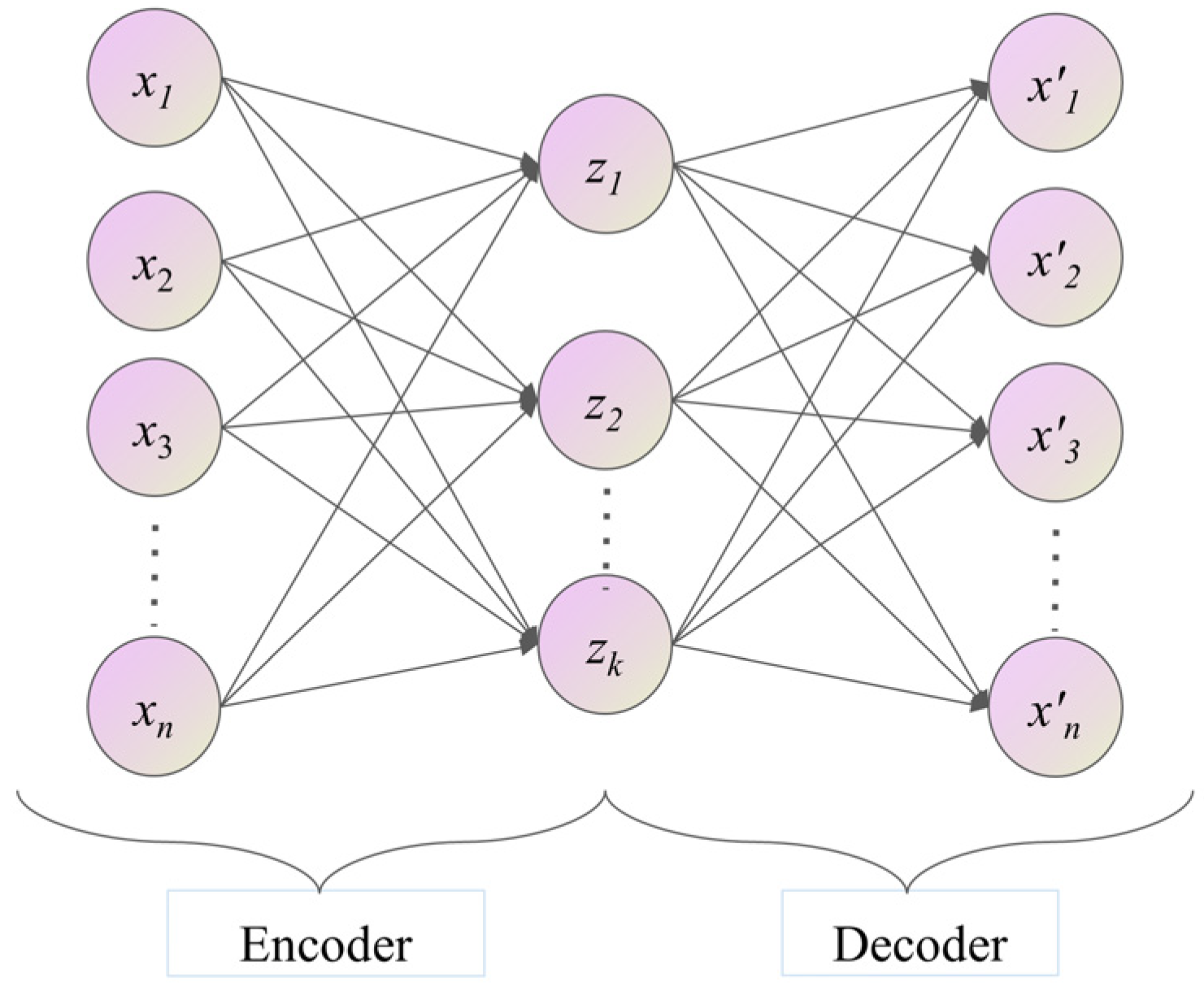
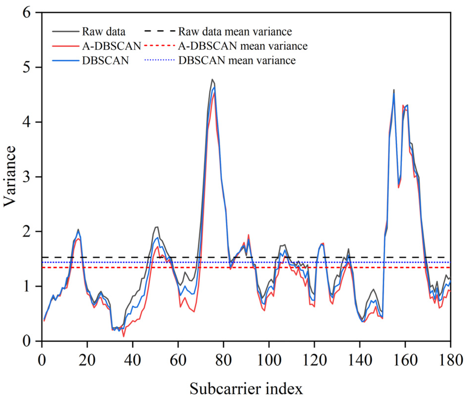
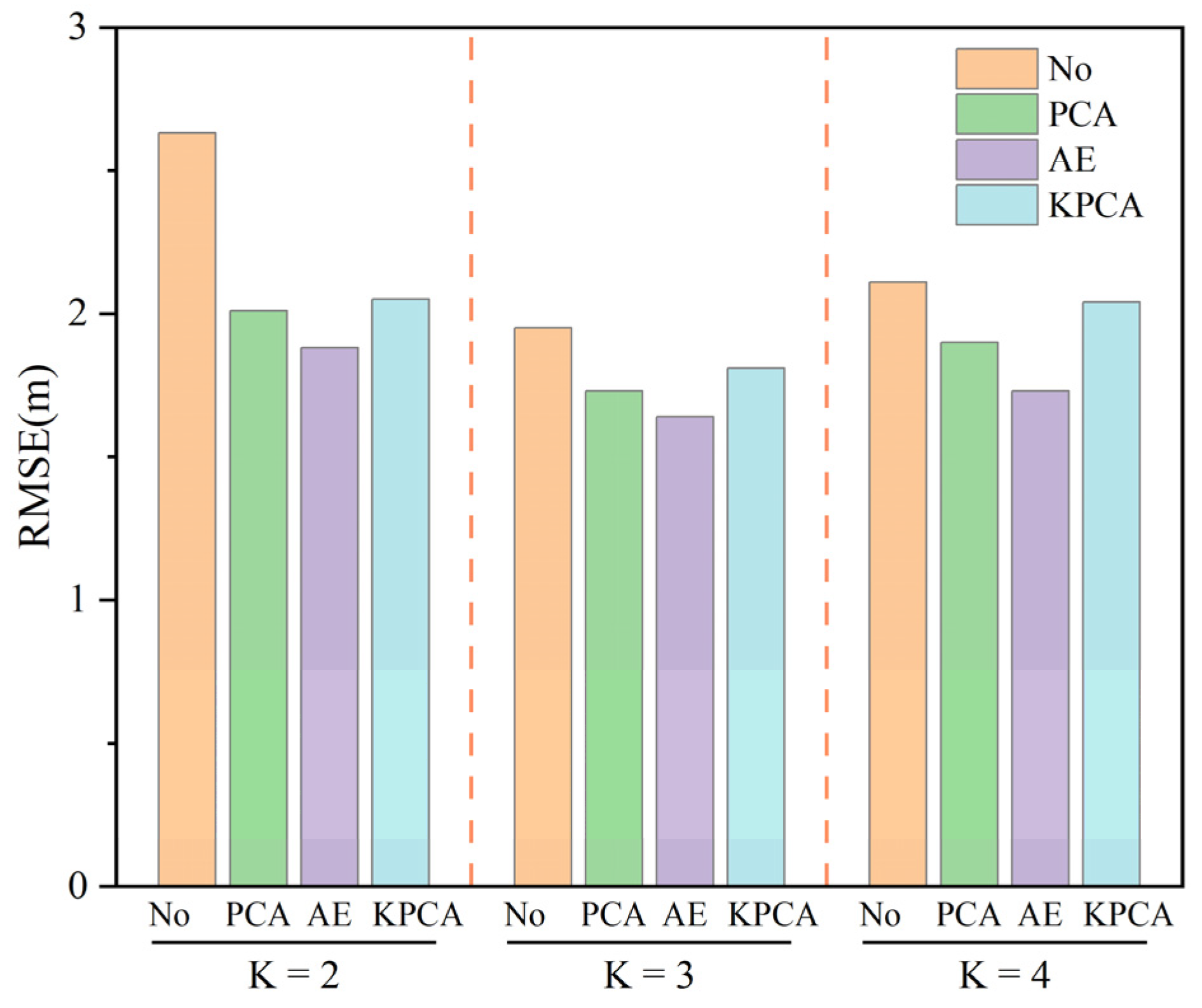
• In the data preprocessing phase, an improved DBSCAN clustering algorithm is proposed for denoising CSI amplitude, and autoencoders are used for feature extraction. These methods’ effectiveness is demonstrated compared with the standard DBSCAN and PCA algorithms.
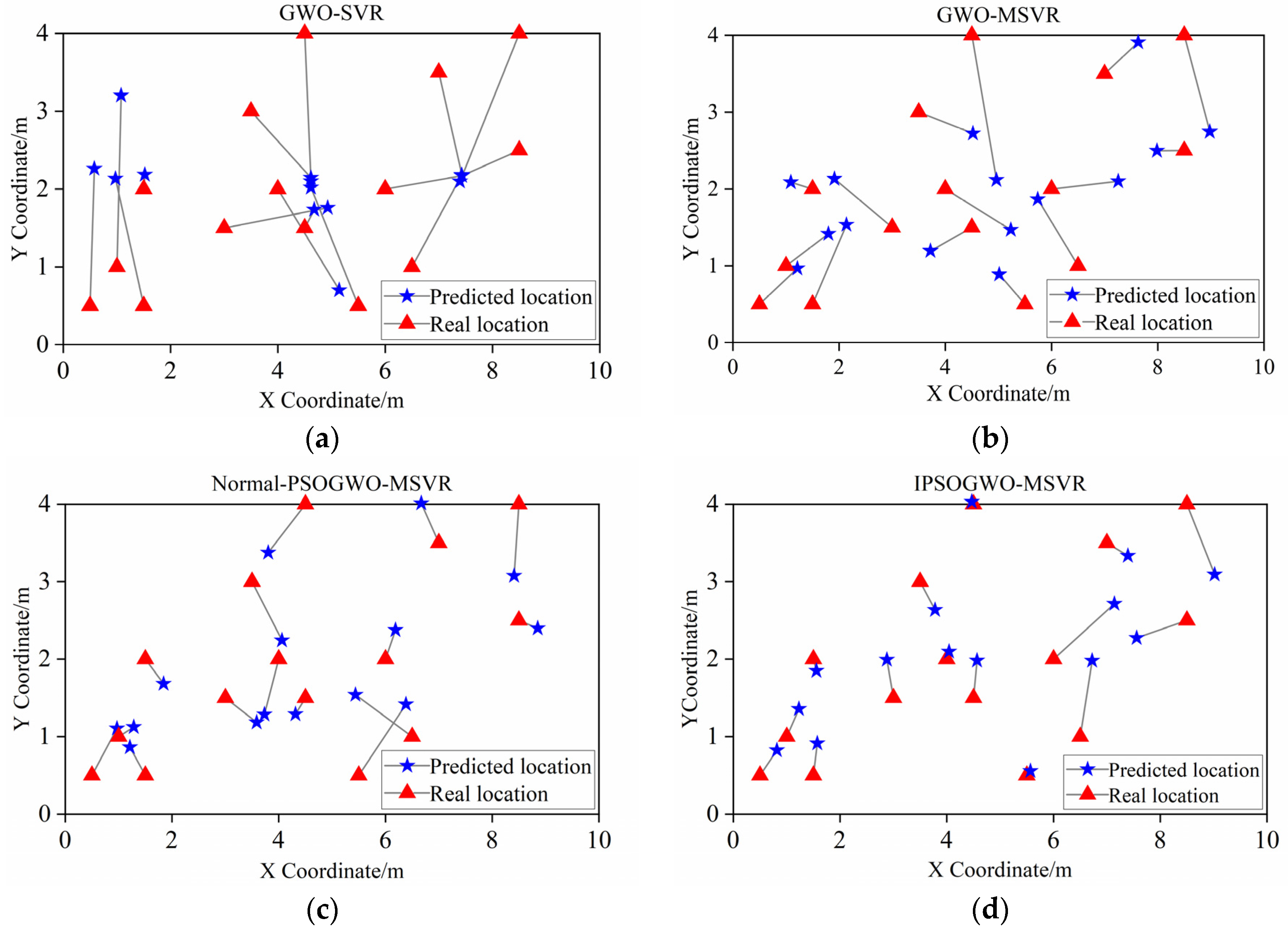
• We employ MSVR for CSI fingerprint localization to bridge the gap in localization efficiency of SVR, and to our knowledge, this is the first time MSVR has been applied in CSI localization.
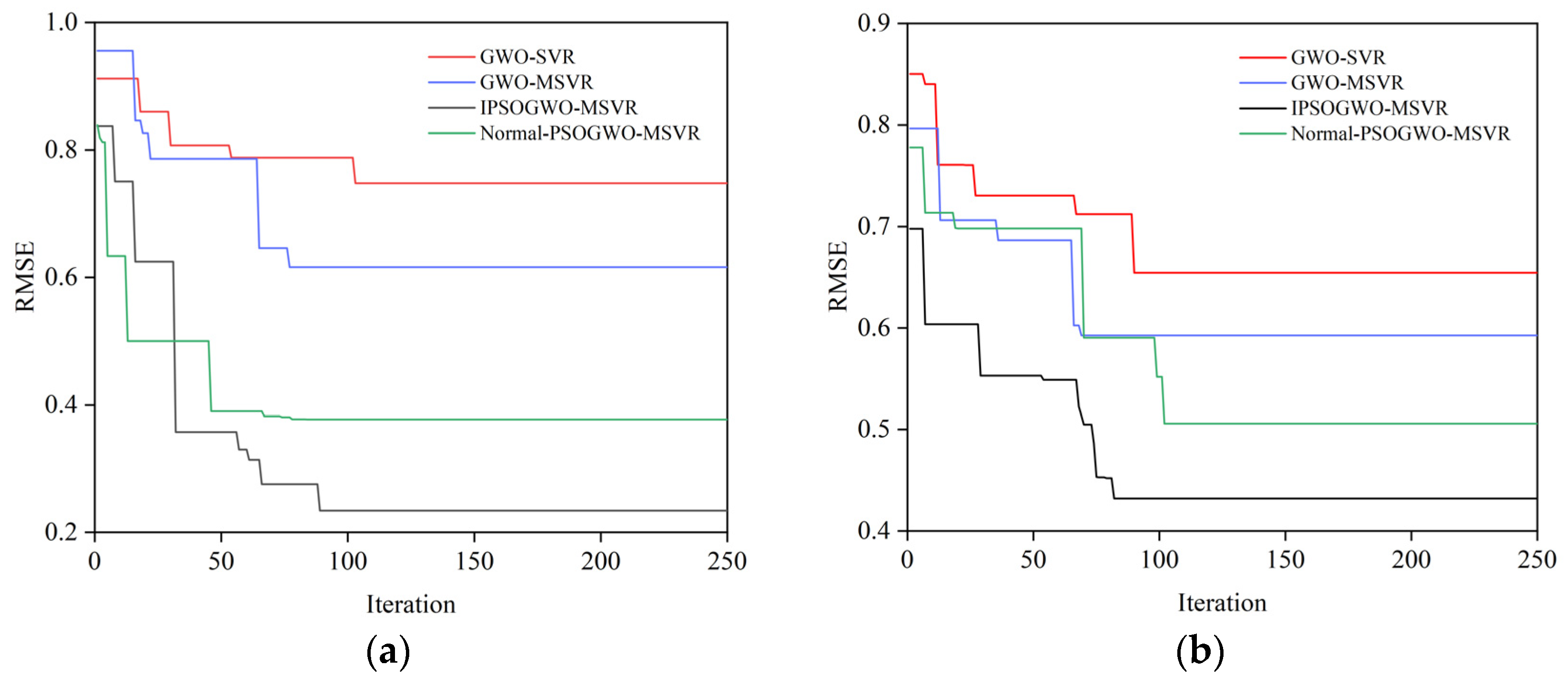
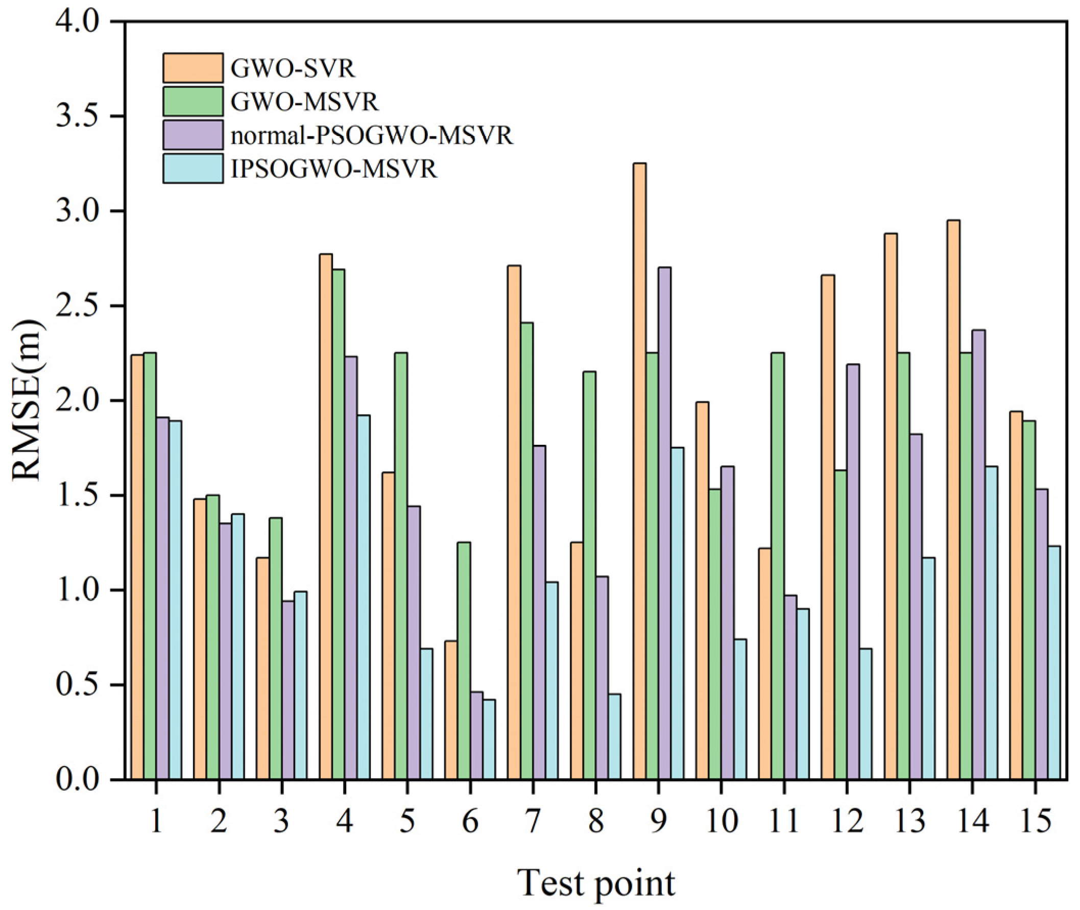
• An improved hybrid optimization algorithm, IPSOGWO, is proposed to adjust the hyperparameters of MSVR to obtain globally optimal parameters. Compared to the unimproved PSOGWO algorithm, the adjusted model can achieve optimal performance.
• The superiority of the proposed method is proven by comparing several domestic and international methods in two scenarios.

The rest of this paper is organized as follows: Section 2 introduces the basic principles of CSI, ADBSCAN, and autoencoders; Section 3 presents the construction of the improved Hybrid Optimization MSVR Localization model; Section 4 introduces the experimental environment and results analysis; Section 5 presents the discussion and conclusions.

2. Framework and Methodologies

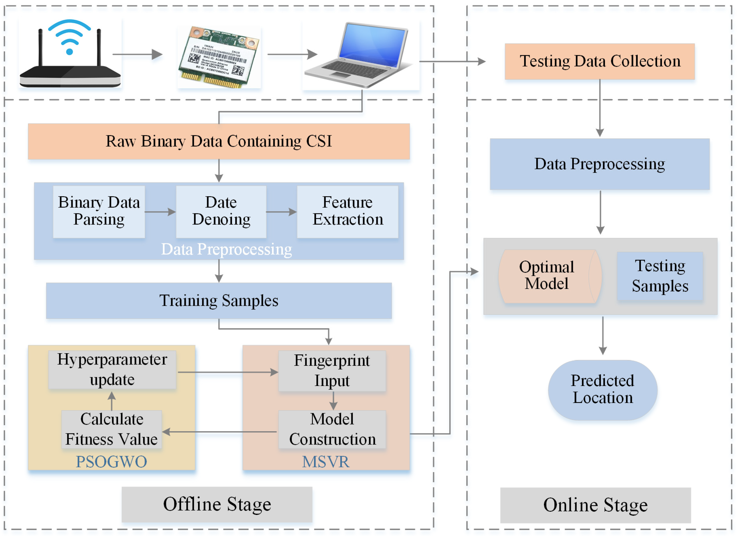
2.1. Systems Framework

This article introduces an improved Hybrid Grey Wolf Particle Swarm Optimization Multi-Output Support Vector Regression (IPSOGWO-MSVR) indoor localization algorithm, as Figure 1 illustrates. Firstly, we utilize the Intel 5300 network interface card to obtain CSI information from Wi-Fi signals. To achieve this goal, we require the support of the Ubuntu 14.04 LTS system and CSI-tools [38] driver program. By enabling the debugging mode on the Intel 5300 network card through CSI-tools, we allow the NIC to report CSI to the main storage. Secondly, we preprocess the collected CSI binary files, including data parsing, denoising, and feature extraction, to mitigate the impact of environmental noise and redundant information on localization results. Subsequently, we construct a CSI location fingerprint database and input it into the PSOGWO-MSVR model for training. The globally optimal parameters obtained from the training are then passed to the online phase, ultimately outputting the optimized model’s localization results.

2.2. Channel State Information

Channel state information (CSI) characterizes the properties of a communication link and falls under the physical layer information of wireless communication protocols. It is employed to describe the fading factor of the signal across each transmission path [39]. When the receiver converting the signal $Y$ transmitted from the sender, the system model in the frequency domain can be expressed as:

$$Y=HX+W$$

(1)

where X is the set of transmit signals, W is the additional Gaussian white noise matrix, and H is the channel transfer matrix, i.e., the CSI matrix:

$$H=\left[H_1,H_2,\cdots ,H_m\right]$$

(2)

According to the IEEE 802.11n/ac standards, when operating at a 20 MHz bandwidth, the Intel 5300 NIC can extract data from 30 subcarriers for each transmit-receive link. Each received H is a complex value, which can be expressed as:

$$H_i=\left|H_i\right|e^{j\sin (\angle H_i)}$$

(3)

where $\left|H_i\right|$ and $\angle H_i$ represent the amplitude and phase information of the i-th subcarrier, respectively. The equipment used in this paper has 2 transmitters and 3 receiver segments, so the data contain 180 subcarriers.

2.3. Noise Reduction

As a popular CSI noise reduction algorithm, DBSCAN clusters objects based on their density in the dataset, identifying anomalies. In the DBSCAN algorithm, we need to pre-set two parameters: the neighborhood radius ε and the density threshold minPts. These parameters generally rely on empirical values [30,40]. However, inappropriate selection of these parameters can impact the noise reduction effect. By analyzing data samples’ structural properties, we introduce A-DBSCAN, a method that adaptively determines parameters for noise reduction. The pseudo-code for Algorithm 1 is as follows:

Algorithm 1: 2–3 uses A-DBSCAN to remove CSI noise

Input: Amplitude information X of a single R-T link, iteration count of K Output: Denoised amplitude X* for i ← 1 to K do  D ← Compute Euclidean Distance Matrix(X);  ε ← Compute Average Distance For INearestNeighbors(D, i);  MinPts ← round(Average Number of Points Within Epsilon(D, ε));  clusters ← DBSCAN(X, ε, MinPts); end for count ← 1; sequence Length ← 10; current Number ← results [1]; best K ← NULL; for i ← 2 to length (results) do;  if results[i] = current Number then   count ← count + 1;  else   count ← 1; current Number ← results[i];  end if  if count = sequence Length then   best K ← i-sequence Length + 1;  end if end for clusters ← DBSCAN (X, ε derived from best K, MinPts derived from best K); Replace noise data in X with average of the remaining data to get X*; return X*;

2.4. Feature Extraction

The original CSI data have high dimensionality and contain a large number of redundant components as well as some valid information. Its direct use for localization can consume excessive computational resources. Furthermore, this approach may affect the localization accuracy. Although PCA is a popular dimensionality reduction method, it is not suitable for complex nonlinear data. In this paper, an autoencoder is used for feature extraction. An autoencoder, an unsupervised neural network model, aims to compress input information, extracting most of the original data content while reducing its dimensionality [41]. A simple autoencoder structure consists of an encoder and a decoder. As shown in Figure 2.

Assuming an input vector $\mathit{x}\in {ℝ}^d$, an encoded vector $\mathit{z}\in {ℝ}^{d\prime }$, and an output vector $\mathit{x}\prime \in {ℝ}^d$, the encoding and decoding processes of the autoencoder can be described as follows:

$$\mathit{z}=\psi ({\mathit{w}}_{encoder}\times \mathit{x}+{\mathit{b}}_{encoder})$$

(4)

$$\mathit{x}\prime =\psi ({\mathit{w}}_{decoder}\times \mathit{z}+{\mathit{b}}_{decoder})$$

(5)

Let $\psi$ denote a nonlinear activation function. In this paper, we employ the hyperbolic tangent function as the activation function for both input and output layers with the following expression:

$$\tanh (x)=\frac{e^x-e^{-x}}{e^x+e^{-x}}$$

(6)

The terms ${\mathit{w}}_{encoder}\in {ℝ}^{d\prime \times d}$ and ${\mathit{b}}_{encoder}\in {ℝ}^{d\prime }$ signify the weights and biases of the encoding layer, respectively. Within the decoding layer, the network endeavors to reconstruct the $d\prime$-dimensional data back into $d$-dimensional form. Here, ${\mathit{w}}_{decoder}\in {ℝ}^{d\times d\prime }$ and ${\mathit{b}}_{decoder}\in {ℝ}^d$ stand for the weights and biases of the decoding layer. The autoencoder utilizes the conventional backpropagation algorithm for weight updates, With the objective of minimizing the root-mean-square error between the input and output, i.e.,

$$L(\mathit{x}-\mathit{x}\prime )={‖\mathit{x}-\mathit{x}\prime ‖}^2$$

(7)

When the total losses are minimized, i.e.,

$$L=\frac{1}{n}{\displaystyle \sum _i^n({‖\mathit{x}-\mathit{x}\prime ‖}^2)}$$

(8)

where n is the number of samples, at which point $\mathit{z}$ emerges as the optimal feature representation of the input data.

3. Improved Grey Wolf Particle Swarm Hybrid Optimization MSVR Localization Model Construction

3.1. Multi-Output Support Vector Regression

Traditional SVR methods for fingerprint localization require modeling and prediction for each dimension separately. This approach is not only inefficient but also overlooks potential connections between outputs. To surmount these limitations, ref. [42] expanded the one-dimensional SVR to handle multi-dimensional outputs, seeking to address more complex challenges found in real-world engineering scenarios. In this study, for training the MSVR algorithm, we use both x and y coordinates of the reference points as well as the gathered signal features. The goal is to construct a regression model that surpasses the traditional SVR in both localization accuracy and localization efficiency.

Let the training sample be denoted as $S=\left\{(x_i,y_i)|i=1,2,\cdots ,K\right\}$, where $x_i\in {ℝ}^M,y_i\in {ℝ}^N$, M, N, and K represent the dimensions of the input signal features, the dimensions of the output reference point coordinates, and the number of samples, respectively. The relationship between the reference point coordinates and the signal features can be described as:

$$\mathit{y}={\mathit{P}}^T\varphi (\mathit{x})+\mathit{B}=\left[\begin{array}{l}{\mathit{w}}_1^T\varphi (x_1)+b_1\\ {\mathit{w}}_2^T\varphi (x_2)+b_2\\ \cdots \\ {\mathit{w}}_N^T\varphi (x_N)+b_N\end{array}\right]$$

(9)

In the equation, $\varphi (\cdot )$ represents the nonlinear mapping in the high-dimensional space, while $\mathit{P}=[w_1,\cdots ,w_j,w_N]$ and $\mathit{B}=[b_1,\cdots ,b_j,b_N]$ are the weight vector matrix and bias, respectively. The MSVR algorithm substitutes the L₁ norm in the traditional single-output SVR’s loss function with an L₂ norm, which is given by:

$$L(u)=\left\{\begin{array}{cc}\hfill 0\hfill & u<\epsilon \hfill \\ \hfill {(u-\epsilon )}^2\hfill & u>\epsilon \hfill \end{array}\right.$$

(10)

where $L(u)$ represents the loss function defined on the hypersphere, with ε being the insensitivity loss domain on the hypersphere. $u_i=‖e_i‖=\sqrt{e_i{}^T{e}_i}$, $e_i=y_i-\mathit{P}\varphi (x_i)-\mathit{B}$. In the case of multi-output regression, Equation (4) is equivalent to the following constraints:

$$\min L(\mathit{P},\mathit{B})=\frac{1}{2}{\displaystyle \sum _{i=1}^N{‖{\mathit{w}}_j‖}^2+C}{\displaystyle \sum _{i=1}^{K}L(u_i)}$$

(11)

where C is the regularization constant, and L represents the ε-insensitive loss function. By introducing the Lagrange multipliers ${\lambda }_i$, we obtain the Lagrangian function as:

$$L(\mathit{P},\mathit{B})=\frac{1}{2}{\displaystyle \sum _{i=1}^N{‖{\mathit{w}}_j‖}^2}+C{\displaystyle \sum _{i=1}^{K}L(u_i)}-{\displaystyle \sum _{i=1}^K{\lambda }_i(u_i{}^2-{‖y_i-\mathit{P}\varphi (x_i)-\mathit{B}‖}^2)}$$

(12)

As the function resides at an extremum, the partial derivatives of $L(\mathit{P},\mathit{B})$ with respect to $p,u,\lambda ,b$ are zero, leading to:

$$\left[\begin{array}{cc}{\varphi }^T{\mathit{D}}_{\alpha }\varphi +\mathit{I}& {\varphi }^T\mathit{\alpha }\\ {\mathit{\alpha }}^T\varphi & {\mathit{I}}^T\mathit{\alpha }\end{array}\right]\left[\begin{array}{c}{w}_j\\ b_j\end{array}\right]=\left[\begin{array}{c}{\varphi }^T{\mathit{D}}_{\alpha }{y}_j\\ {\mathit{\alpha }}^T{y}_j\end{array}\right]$$

(13)

where $\varphi ={\left[\varphi (x_1),\cdots ,\varphi (x_K)\right]}^T$, ${\mathit{D}}_{\alpha }=diag({\alpha }_1,\cdots ,{\alpha }_K)$, $\mathit{\alpha }={\left[{\alpha }_1,\cdots ,{\alpha }_K\right]}^T$, $\mathit{I}={\left[1,\cdots ,1\right]}^T$. Expressing $w_j$ as a linear combination of samples in the feature space, i.e., $w_j={\displaystyle \sum \varphi (x_i){\beta }_i^j}={\varphi }^T{\beta }^j$, and substituting into Equation (13), we obtain the following expression:

$$\left[\begin{array}{cc}\mathit{K}+{\mathit{D}}_{\alpha }^{-1}& \mathit{I}\\ {\mathit{\alpha }}^T\mathit{K}& {\mathit{I}}^T\mathit{\alpha }\end{array}\right]\left[\begin{array}{c}{\beta }^j\\ b_j\end{array}\right]=\left[\begin{array}{c}{y}_j\\ {\mathit{\alpha }}^T{y}_j\end{array}\right]$$

(14)

where $\mathit{K}={\mathit{K}}_{ij}={\varphi }^T(x_i)\varphi (x_j)$ is a kernel function. Research has shown that, in the absence of prior knowledge, the use of the radial basis kernel function to map data from a low-dimensional space to a high-dimensional space yields promising results [43]. The expression is given as follows:

$${\mathit{K}}_{ij}=exp(-\frac{{‖x_i-x_j‖}^2}{2{\sigma }^2})$$

(15)

By iteratively determining $\mathit{\beta }=\left[{\beta }^1,\cdots ,{\beta }^K\right]$, the output coordinates can be expressed as:

$$\mathit{y}={\varphi }^T(\mathit{x})\varphi (\mathit{x})\mathit{\beta }={\mathit{K}}_{ij}\mathit{\beta }$$

(16)

From our derivation, it is clear that MSVR’s regression performance depends on three hyperparameters: the regularization constant C, the insensitivity loss coefficient γ, and the kernel function radius σ. Consequently, we use intelligent optimization algorithms to find the optimal values for these parameters: C, γ, and σ.

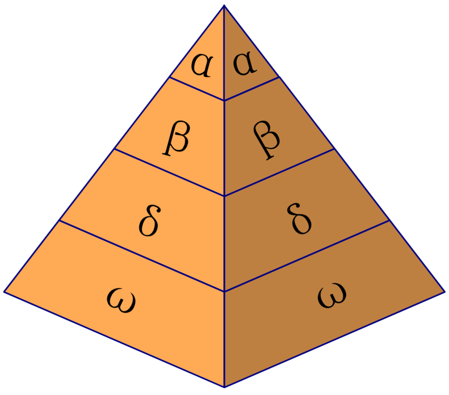
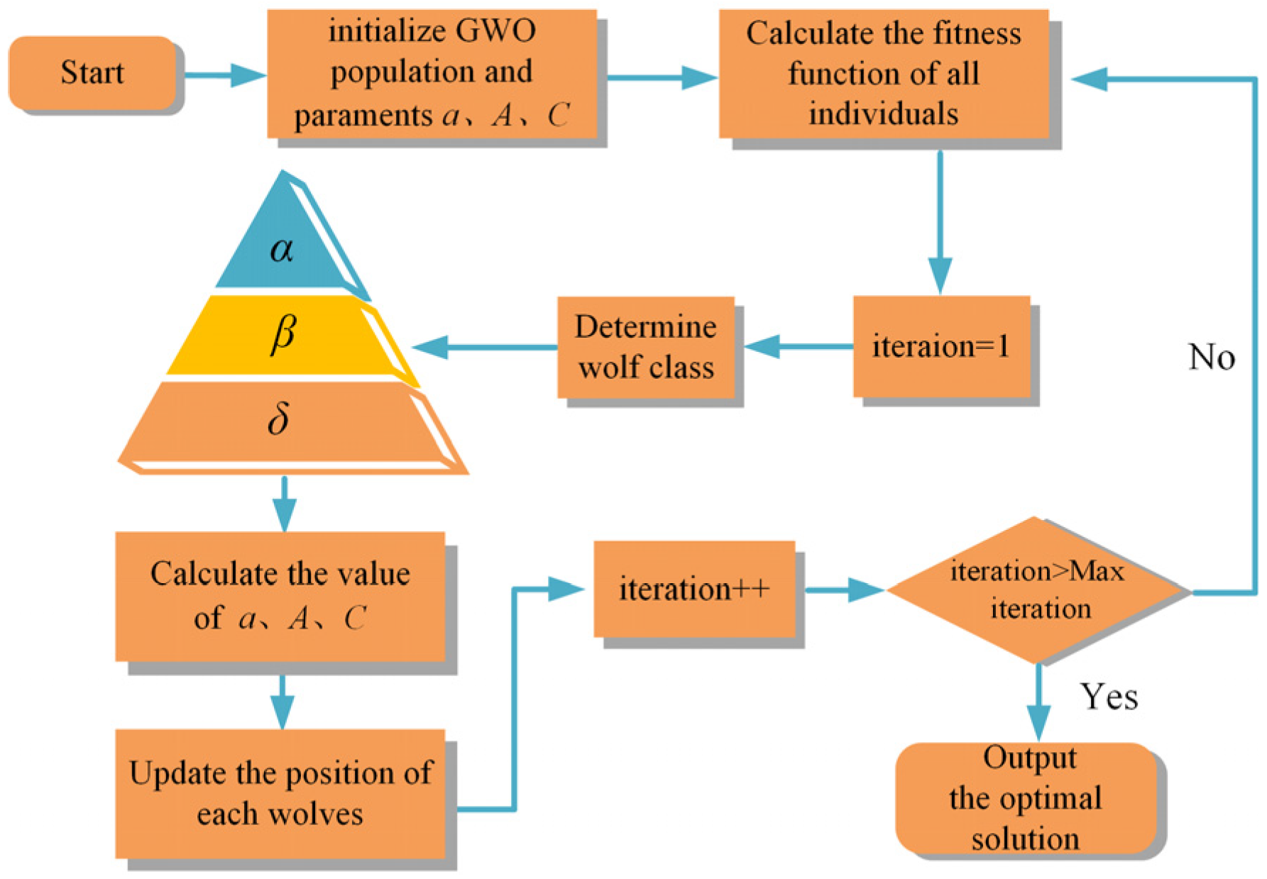
3.2. Grey Wolf Optimization Algorithm

The Grey Wolf Optimization (GWO) algorithm draws inspiration from the predatory behavior and social hierarchy observed in grey wolves [44]. Figure 3 depicts this societal structure of a wolf pack. At the pinnacle are the α wolves, who lead the pack in hunting and decision-making. The β wolves form the second tier, supporting and assisting the α wolves in their endeavors. Next in the hierarchy are the δ wolves, responsible for transmitting the decisions of the higher-ranking wolves. Finally, the ω wolves, situated at the lowest tier, follow the commands of the other members. This collaborative structure enables the wolf pack to effectively carry out its hunting activities.

The primary objective of the Grey Wolf Optimization algorithm is to obtain the optimal solution for parameters, analogous to capturing prey. Therefore, before the hunt begins, the wolf pack first determines an approximate location of the prey, followed by encirclement. The mathematical model for this behavior is expressed as:

$$\mathit{d}=\left|\mathit{C}\times {\mathit{X}}_p(i)-{\mathit{X}}_g(i)\right|$$

(17)

$${\mathit{X}}_g(i+1)={\mathit{X}}_p(i)-\mathit{A}\times \mathit{d}$$

(18)

In the equation above, ${\mathit{X}}_p(i)$ and ${\mathit{X}}_g(i)$ denote the positions vectors of the prey and the grey wolf at the i-th iteration, respectively. $\mathit{d}$ is the distance between them, while $\mathit{A}$ and $\mathit{C}$ are coefficient vectors, which are determined as follows:

$$\left\{\begin{array}{l}\mathit{A}=2\mathit{a}\cdot {\mathit{r}}_1-\mathit{a}\\ \mathit{C}=2{\mathit{r}}_2\\ \mathit{a}=2\left(1-i/I_{\max }\right)\end{array}\right.$$

(19)

where ${\mathit{r}}_1$ and ${\mathit{r}}_2$ are random vectors within [0, 1], I_max represents the maximum number of iterations, and $a$ decreases linearly from 2 to 0 as the number of iterations increases. Once the wolves complete their encirclement of the prey, they initiate an attack. Depending on the prey’s location, the positions of the grey wolves at all hierarchical levels will adjust. The specific updated strategies are as follows:

$$\left\{\begin{array}{l}{\mathit{d}}_{\mathit{\alpha }}=\left|{\mathit{C}}_1\times {\mathit{X}}_{\alpha }(i)-{\mathit{X}}_p(i)\right|\\ {\mathit{d}}_{\beta }=\left|{\mathit{C}}_1\times {\mathit{X}}_{\beta }(i)-{\mathit{X}}_p(i)\right|\\ {\mathit{d}}_{\delta }=\left|{\mathit{C}}_1\times {\mathit{X}}_{\delta }(i)-{\mathit{X}}_p(i)\right|\end{array}\right.$$

(20)

$$\left\{\begin{array}{l}{\mathit{X}}_1(i)=\left|{\mathit{X}}_{\alpha }(i)-{\mathit{A}}_1\times {\mathit{d}}_{\alpha }\right|\\ {\mathit{X}}_2(i)=\left|{\mathit{X}}_{\beta }(i)-{\mathit{A}}_2\times {\mathit{d}}_{\beta }\right|\\ {\mathit{X}}_3(i)=\left|{\mathit{X}}_{\delta }(i)-{\mathit{A}}_3\times {\mathit{d}}_{\delta }\right|\end{array}\right.$$

(21)

$$\mathit{X}(i+1)=\frac{{\mathit{X}}_1(i)+{\mathit{X}}_2(i)+{\mathit{X}}_3(i)}{3}$$

(22)

Using Equation (20), the distances of other wolves from α, β, and δ are calculated. Equation (21) determines the moving directions of the remaining grey wolf individuals. Their positions are then updated according to Equation (22). As the iterations proceed, the wolf pack eventually completes the hunt, with the final position of the α wolf signifying the optimal parameters. Figure 4 illustrates the optimization process of the Grey Wolf algorithm.

3.3. The IPSOGWO Model

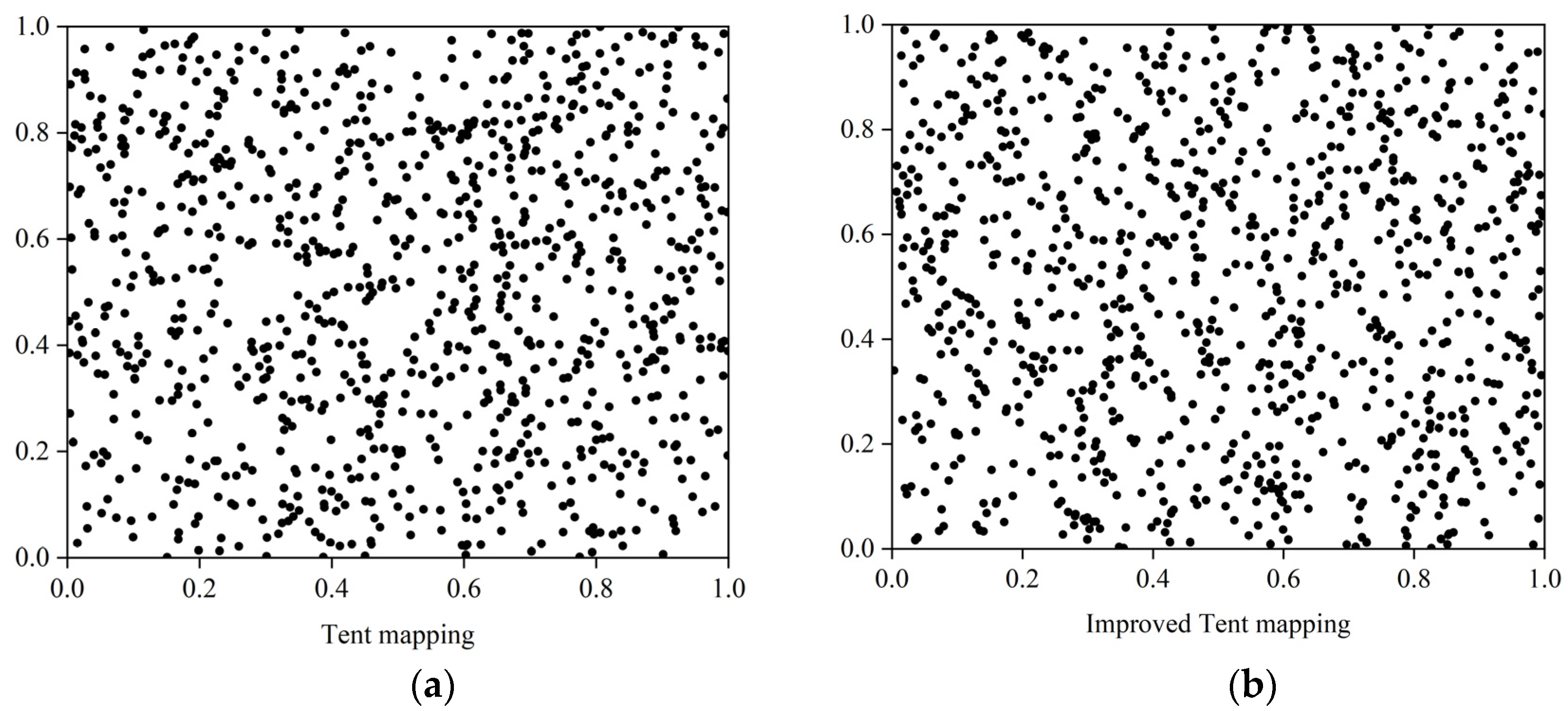
3.3.1. Improved Tent Chaos Mapping

The efficacy of intelligent swarm algorithms is largely influenced by the spatial distribution of the population after initialization. However, traditional GWO algorithms randomly generate the initial population, which may not ensure a uniform distribution in the search space. To address this, we suggest employing chaotic mapping for the initial population generation of grey wolves. The Tent map, while effective in chaotic sequences, grapples with issues such as indeterminate periodic points [45]. Given that the initial population should exhibit a thoroughly randomized nature, we incorporate a random variable r/N into the traditional Tent map. The modified expression for the Tent map is presented below:

$$x_{i+1}=\left\{\begin{array}{ll}2x_i+r/N& x_i\in [0,0.5]\\ 2(1-x_i)+r/N& x_i\in (0.5,1]\end{array}\right.$$

(23)

where N is population size, and r is random number within [0, 1]. The chaotic values can be obtained through Equation (23), which is then mapped to the population search space, i.e.,

$$\begin{array}{l}{y}_i=lb+x_i\times (ub-lb)\\ st.\left\{\begin{array}{ll}{y}_i=ub& y_i>ub\\ y_i=lb& y_i<lb\end{array}\right.\end{array}$$

(24)

In the above equation, ub and lb refer to the upper and lower bounding ranges of the grey wolf location, respectively. Figure 5 displays the distribution after Tent mapping. The original Tent mapping tends to cause a pile-up phenomenon in certain areas, while the improved Tent mapping distributes points more uniformly.

3.3.2. Improved Location Updating Strategy

In the grey wolf optimization algorithm’s position update process, the method focuses on information exchange between individual wolves and the population. It neglects each wolf’s relationship with its historical position. Ref. [46] introduced an enhanced GWO algorithm that incorporates concepts from Particle Swarm Optimization. The position update strategy for the wolves in this hybrid algorithm is as follows:

$${\mathit{X}}_i(i+1)=c_1{r}_3(w_1{\mathit{X}}_1(t)+w_2{\mathit{X}}_2(t)+w_3{\mathit{X}}_3(t))+c_2{r}_4({\mathit{X}}_{ibest}-{\mathit{X}}_i(i))$$

(25)

In Equation (25), $c_1$ is the social learning factor and $c_2$ is the cognitive learning factor. These values respectively indicate how the individual’s best experience and the swarm’s best value influence the algorithm’s search direction. Both $r_3$ and $r_4$ are random variables within [0, 1]. ${\mathit{X}}_{ibest}$ denotes the historically best position that a particular wolf has encountered. The terms $w_1$, $w_2$, and $w_3$ adjust the weights of α, β, and δ to help the algorithm avoid local optima. They are determined by the following equation:

$$\left\{\begin{array}{l}{w}_1=\frac{\left|{\mathit{X}}_1\right|}{\left|{\mathit{X}}_1+{\mathit{X}}_2+{\mathit{X}}_3\right|}\\ w_2=\frac{\left|{\mathit{X}}_2\right|}{\left|{\mathit{X}}_1+{\mathit{X}}_2+{\mathit{X}}_3\right|}\\ w_3=\frac{\left|{\mathit{X}}_3\right|}{\left|{\mathit{X}}_1+{\mathit{X}}_2+{\mathit{X}}_3\right|}\end{array}\right.$$

(26)

Incorporating concepts from Particle Swarm Optimization has undoubtedly improved the algorithm’s optimization capabilities. However, the authors in [46] assigned constant values to $c_1$ and $c_2$. They neglected that the weights of the learning factors should adjust dynamically with each iteration. To address this, our study introduces a grey wolf position update strategy with adaptive learning factors. Instead of being fixed, the modified learning factors $c_1$ and $c_2$ adjust complementarily: as $c_1$ decreases, $c_2$ increases. This method ensures a balance between global search capability and enhanced local search ability. The equation is presented as follows:

$$\left\{\begin{array}{l}{c}_1=c_1(\max )-\frac{(c_1(\max )-c_1(\min ))\cdot i}{I}\\ c_2=c_2(\min )+\frac{(c_2(\max )-c_2(\min ))\cdot i}{I}\end{array}\right.$$

(27)

Substituting this into Equation (25) yields the final position updated equation.

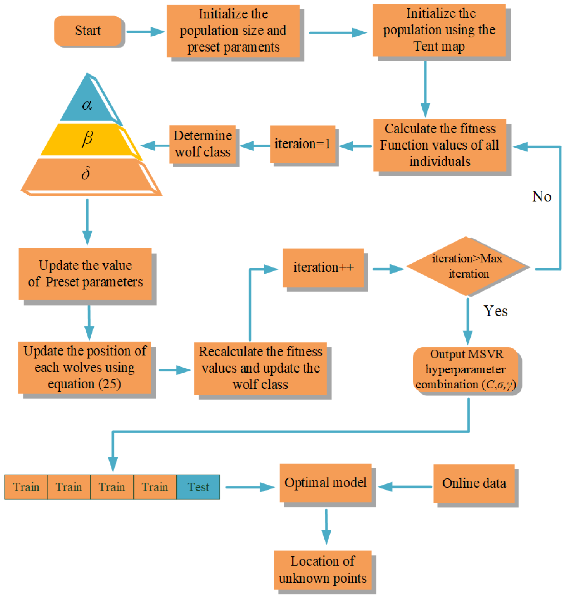
3.3.3. IPSOGWO-MSVR Positioning Model

The whole process of localization of the IPSOGWO-MSVR algorithm proposed in this paper is as follows:

Step 1 involves initializing algorithm parameters: setting the population size to 30, the number of iterations to 250, C to 0.1–100, γ to 0.01–100, σ to 0.01–1, social learning factors $c_1(\max )$ and $c_2(\max )$ to 2.05, and cognitive learning factors $c_1(\min )$ and $c_2(\min )$ to 1.1.

Step 2 involves generating the initial population based on the improved Tent mapping, while simultaneously calculating the fitness values of the population individuals. The grey wolf ranks are determined by the three highest fitness values. The root-mean- square error is chosen as the fitness function for parameter optimization in this article:

$$\mathrm{RMSE}=\sqrt{\frac{{\displaystyle {\sum }_{i=1}^K({\displaystyle {\sum }_{j=1}^N{(y_{i,j}-{\tilde{y}}_{i,j})}^2})}}{K}}$$

(28)

where $y$ and $\tilde{y}$ represent the actual coordinates and the coordinates predicted by the model, respectively.

Step 3 involves calculating and updating A and C according to Formula (19) and updating the positions of the grey wolves according to Formula (25). The fitness values are then recalculated, and the grey wolf ranks are updated.

Step 4 is the termination criterion. The algorithm terminates once it reaches the maximum number of iterations, returning the globally optimal parameter combination (C, γ, σ). Otherwise, steps 2–4 are repeated.

Step 5 involves the MSVR conducting five-fold cross-validation training on the database according to the optimal parameter combination, outputting the optimal model, and predicting the target location based on the fingerprints during the online phase.

The specific process is depicted in the following Figure 6.

4. Experiments and Results Analysis

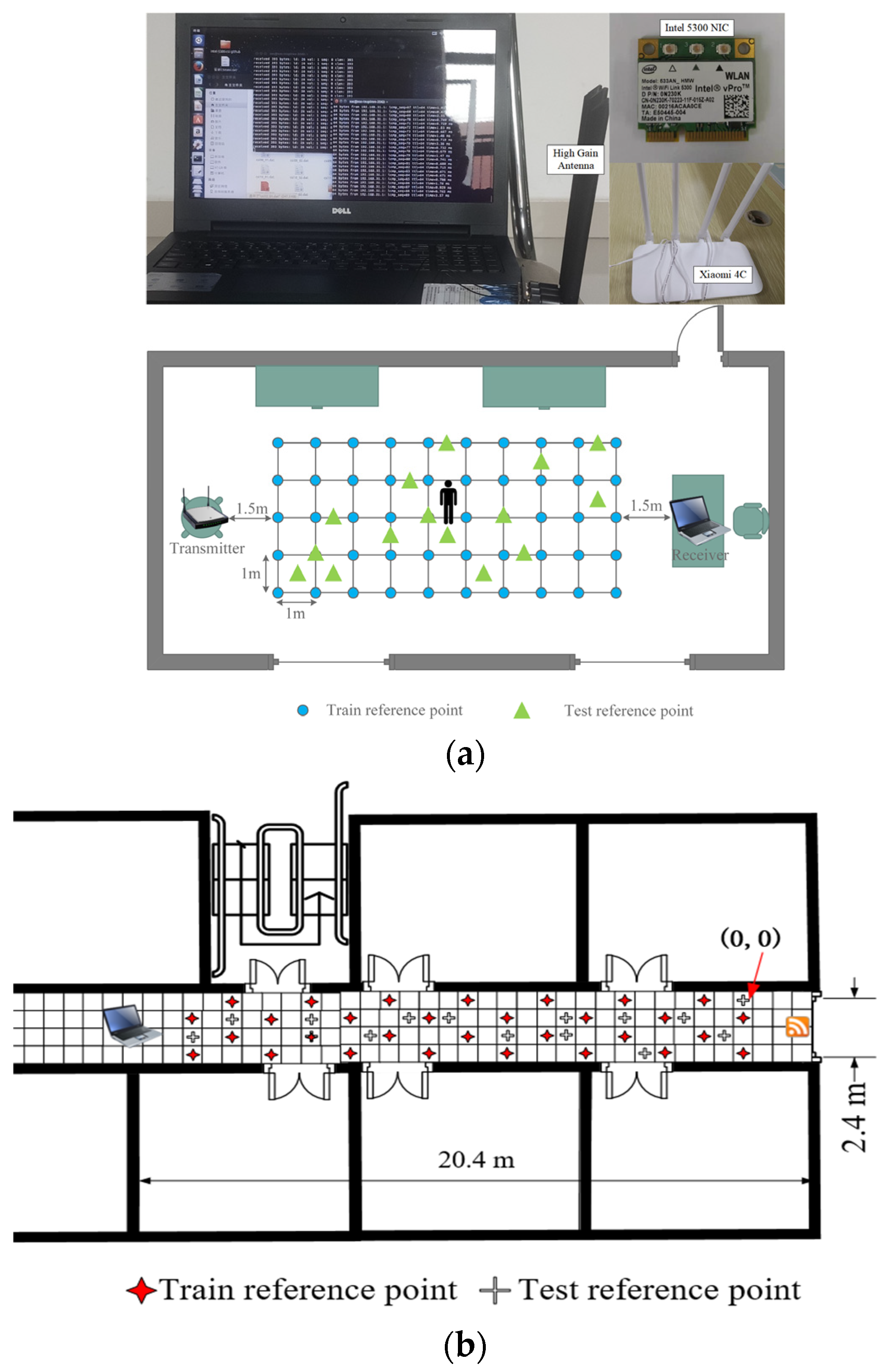
4.1. Data Collection

We selected two areas under LOS (line of sight) scenarios for the experiments. The first experimental scenario has an area of approximately 9 × 4 m², with 50 reference points and 15 test points, totaling 65 points. In Figure 7a, reference points are represented by blue solid circles, and test points by green triangles. The reference points are 1 m apart, with the bottom-left corner as the coordinate origin, defining coordinates for each point. The second experimental scenario is a narrow corridor area, measuring approximately 20.4 × 2.4 m², with 30 reference points and 15 test points selected, totaling 45 points. In Figure 7b, reference points are denoted by stars and test points by crosses. A Xiaomi 4C router is used as the access point (AP). A Dell Inspiron 3543 laptop, equipped with an Intel 5300 network card and version 4.2 of the CSI-tools software, serves as the data collection platform. It runs on the Ubuntu 14.04 LTS operating system. The AP is positioned at a height of 0.5 m above the ground, and the data collection platform at a height of 0.8 m, with both devices located approximately 1.5 m outside the experimental area. The collection frequency is set to 10 Hz, with the experimenters standing still at each point for 20 s, collecting 200 samples.

Table 1. Configuration parameters of experimental equipment.

Specifications	Transmitter	Receiver
Network Standard	IEEE 802.11 b/g/n
Maximum Transmission Rate	300 Mbps
Operating Band	2.4 GHz
Number of Antennas	4	3
MIMO Mode	2 × 2 MIMO	2 × 3 MIMO

shows the detailed parameters of the transmitting and receiving devices.

4.2. Comparison of Preprocessing Methods

To verify the effectiveness of the improved denoising algorithm, we apply A-DBSCAN denoising to 180 subcarriers, calculate the variance of each subcarrier after denoising, and compare it with the variance of the original data and the variance after standard DBSCAN denoising. As Figure 8 shows, after executing the A-DBSCAN algorithm for denoising, the variance of the CSI subcarriers is significantly reduced. The dashed line in Figure 8 represents the average variance of the 180 subcarriers, where A-DBSCAN is 1.343, outperforming the standard DBSCAN’s 1.450 and the original data’s 1.531, proving that the A-DBSCAN algorithm can effectively remove the noise from the original CSI amplitude.

We take the noise-reduced CSI amplitude as input and use AE for dimensionality reduction. In our tests, the error from the 20-dimensional features extracted by AE was only 0.15%. This result shows that the extracted low-dimensional features already contain most of the relevant information. Therefore, we choose 20-dimensional data to construct fingerprints.

To assess the performance of our dimensionality reduction technique, we juxtaposed it with two well-established methods, PCA and KPCA. We subjected the CSI amplitude data, gathered during the offline phase, to each of these three methods. Using the dimensionally reduced feature sets combined with the coordinates of reference points, we formulated position fingerprints $F_i=\{(P_i,(x_i,y_i)\}$, where $P=\{p_1,\cdots ,p_j\}$ stand for the reduced feature sets with components, while $(x_i,y_i)$ signifies the position label. We used these fingerprints to create a database. Subsequently, data procured during the online phase were processed similarly, with positioning executed using the KNN algorithm.

Table 2. Parameters chosen for the three dimensionality reduction algorithms.

Reduction Algorithms	Parameters	Value
AE	Coding dimension	20
	Iterations	200
	Activation functions (encoding and decoding layers)	tanh
	Adam optimizer learning rate	0.01
	Loss function	MSE
PCA	Variance explained/number of principal components	99%/74
KPCA	Kernel function	RBF
	Variance explained/number of principal components	99%/110

provides the parameter settings for the three dimensionality reduction methods used in the experiments of this paper.

Figure 9 shows the positioning results from which we observe that the root-mean- square error (RMSE) for the KNN algorithm is consistently highest when using data without dimensionality reduction, regardless of the chosen value for K. Specifically, when K = 3 (where the KNN algorithm performs optimally), the RMSE value for the unprocessed data is 1.95 m. For data processed with the three dimensionality reduction techniques, the values are 1.73 m, 1.65 m, and 1.81 m, respectively. This demonstrates that using dimensionality-reduced data provides better positioning accuracy compared to the direct use of raw data.

Theoretically, CSI data are understood to exhibit a high degree of nonlinearity, suggesting that nonlinear dimensionality reduction methods might offer better results. Yet, according to this study’s outcomes, the KPCA algorithm consistently underperforms compared to PCA, both in dimensionality reduction and positioning phases. Such underperformance could stem from the tendency of nonlinear kernels to over-fit, which in turn affects the overall performance. Furthermore, the selected kernel parameters might not be the most suitable. On the other hand, the autoencoder, another nonlinear dimensionality reduction method, showcased the best results in our tests. This implies that employing this approach to process raw CSI data can effectively diminish data complexity, thereby boosting the system’s operational efficiency and positioning accuracy.

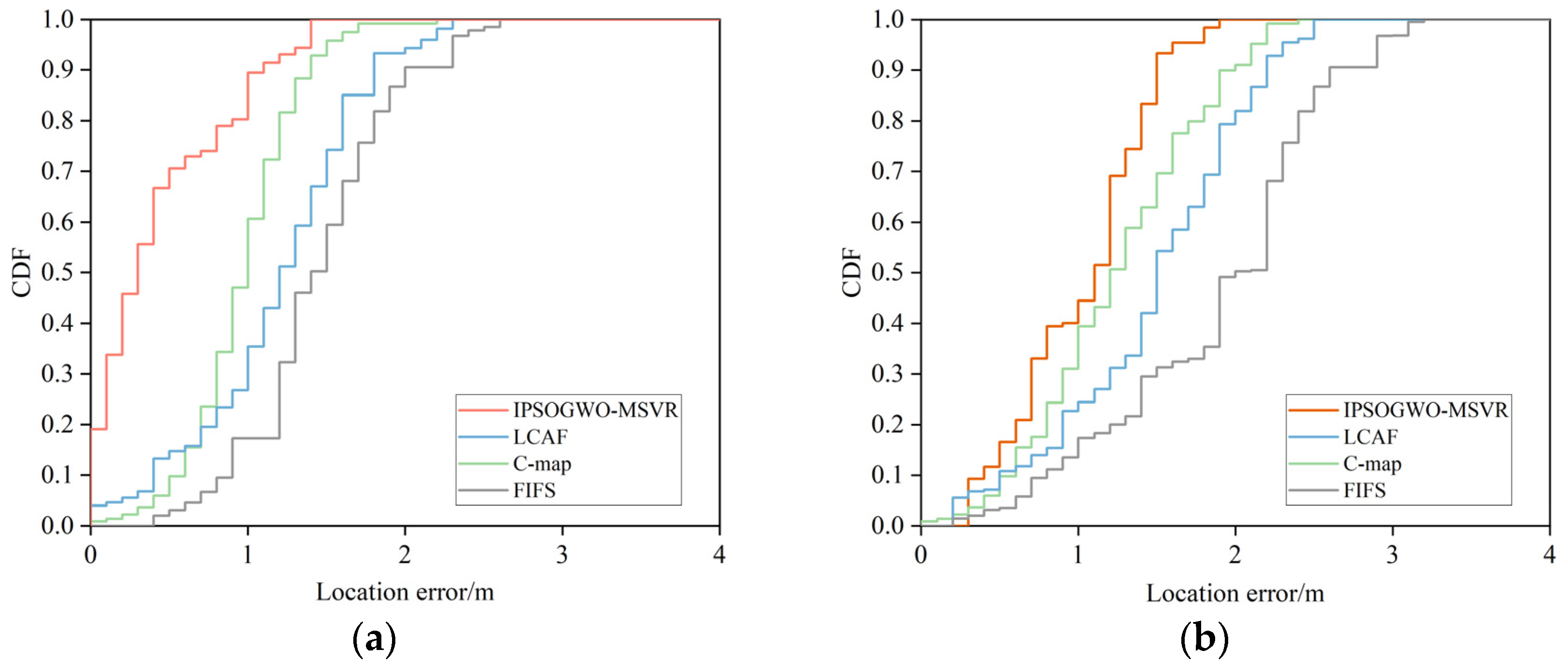
4.3. Comparison with Similar Location Methods

To evaluate the performance of the IPSOGWO-MSVR localization algorithm, we compare it with three methods. These methods are GWO-SVR, GWO-MSVR, and a hybrid optimization algorithm without improvements, which we refer to as normal-PSOGWO-MSVR. The preset parameters for the different methods are consistent with IPSOGWO-MSVR, as Section 3.3.3 describes. After 250 iterations of training, Figure 10 illustrates the RMSE trends of the four methods in the two scenarios.

As Figure 10 shows, the RMSEs of the GWO-SVR and GWO-MSVR algorithms are relatively high in both scenarios after the iterations have converged. Specifically, their values are 0.747, 0.613, and 0.654, 0.592 for the two scenarios, respectively. This indicates that whether it is SVR or MSVR, the efficiency of using a single algorithm for parameter optimization is low. Moreover, it is prone to falling into local optima and cannot escape. However, the RMSEs of the two algorithms reveal that MSVR’s predictions are superior to SVR’s. A smaller RMSE indicates that the predicted target points by the algorithm are closer to the actual values. This also demonstrates that using MSVR in place of SVR as a localization algorithm is feasible. From the convergence curves in both scenarios, the post-convergence RMSEs of IPSOGWO-MSVR and normal-PSOGWO-MSVR algorithms are notably lower than those utilizing single optimization methods. Specifically, they are 0.232, 0.43, and 0.377, 0.508, respectively. However, the local search capability of normal-PSOGWO-MSVR is not as good as that of IPSOGWO-MSVR, with the latter being able to escape local optima to achieve a smaller RMSE. It can be concluded from the figure that IPSOGWO-MSVR has stronger optimization capabilities.

Table 3. Configuration of initialization parameters and optimal parameter combinations.

Scenarios	Value	C	σ	γ
Scenarios 1	GWO-SVR	0.1	0.1	0.04
	GWO-MSVR	0.1	0.1	0.66
	IPSOGWO-MSVR	0.1	11.8	0.23
	Normal-PSOGWO-MSVR	0.1	9.7	0.62
Scenarios 2	GWO-SVR	0.3	0.1	0.05
	GWO-MSVR	0.2	0.1	0.71
	IPSOGWO-MSVR	0.2	8.1	0.47
	Normal-PSOGWO-MSVR	0.3	7.5	0.86

shows the optimal parameter combinations of the four models in the two scenarios.

The optimal hyperparameter combinations determined by each of the four methods were applied to the model training, and then the data collected during the localization phase were pre-processed in the same way before being input into the model to obtain the final prediction results, as Figure 11 and Figure 12 show.

Figure 11 and Figure 12 show that the improved PSOGWO-MSVR algorithm outperforms the other three in both scenarios. In Scenario 1, the prediction results of most of the test points are close to the real position and evenly distributed. In Scenario 2, the average RMSE of the 15 test points for the four algorithms are as follows: 2.05 m, 1.99 m, 1.62 m, and 1.12 m. Notably, the RMSE of the improved PSOGWO-MSVR remains below 1.5 m. It can be seen that the localization model constructed by Multi-Output Support Vector Regression is more accurate relative to the single-output regression model. This is because the multi-output model considers the intrinsic connection between output variables. It treats errors holistically during training, achieving an optimal fit for each component. In contrast, the single-output model handles each component’s output separately, amplifying errors upon combination and reducing localization accuracy.

4.4. Comparison of Advanced Positioning Techniques

We compare the IPSOGWO-MSVR algorithm with FIFS, C-map, and LCAF. This is because they all solely use CSI amplitude as the fingerprint for localization. The detailed processing procedures of the comparison methods can be found in [19,47,48].

Table 4. Comparison of root-mean-square errors across four methods.

Scenarios	Method	Maximum Error (m)	Minimum Error (m)	Mean Error (m)
Scenario 1	FIFS	2.61	0.47	1.50
	C-map	2.07	0.18	1.03
	LCAF	2.21	0.36	1.24
	PSOGWO-MSVR	1.35	0.11	0.59
Scenario 2	FIFS	3.27	0.42	2.20
	C-map	2.44	0.33	1.34
	LCAF	2.56	0.32	1.58
	PSOGWO-MSVR	1.92	0.41	1.12

presents the error statistics for the four localization methods in two experimental scenarios.

Table 4 shows that in Scenario 1, the average localization error of the algorithm proposed in this paper is 0.59 m. Compared with FIFS, C-map, and LCAF algorithms, the average localization accuracy is improved by 60.7%, 42.7%, and 52.4%, respectively. In Scenario 2, the average localization error of the algorithm proposed in this paper is 1.12 m, with accuracy improvements of 45.4%, 29.1%, and 16.4% compared to the other three algorithms, respectively. We also note that the overall localization accuracy in Scenario 2 is lower than in Scenario 1, with the error rates of various algorithms respectively increasing by 46.7%, 30%, 27.4%, and 89.8%.

Figure 13 shows the localization cumulative probability distribution function (CDF) of the four methods in two scenarios. In Scenario 1, with an error threshold of 1 m, the CDF value for IPSOGWO-MSVR is 80.3%. In comparison, FIFS, LCAF, and C-map have values of 17.3%, 26.8%, and 47%, respectively. This indicates that the majority of our algorithm’s localization errors are less than 1 m. In Scenario 2, with a threshold of 1.5 m, FIFS, LCAF, and C-map report CDF values of 29.5%, 42%, and 62.9%, respectively. Meanwhile, IPSOGWO-MSVR achieves 79.8%. From the error statistics and CDF comparison, our proposed IPSOGWO-MSVR algorithm outperforms the other three methods.

5. Discussion and Conclusions

5.1. Discussion

Through the experimental results in Section 4.3, it is clear that MSVR can effectively improve the localization accuracy compared with SVR regression. Meanwhile, the improved IPSOGWO algorithm reduces the average localization error by 26.1% and 30.9% in the two scenarios compared to the standard PSOGWO algorithm. This indicates that the improved algorithm can find the optimal grey wolf individuals in iterations, providing globally optimal parameters for MSVR. The experimental results in Section 4.4 show that the performance of the IPSOGWO-MSVR algorithm is still the best among the four methods, but we notice that the error of the IPSOGWO-MSVR algorithm rises more after switching from Scenario 1 to Scenario 2. We analyze that a possible reason for the increased error is the greater distance between the transmitter and receiver devices in Scenario 2. Additionally, the signal carries more ambient noise after reflecting from the multipath, affecting the model’s localization performance, indicating that our algorithm’s ability to resist the multipath is still relatively weak. In our next study, we will focus on the modeling of the localization performance of the model and work on improving its stability, incorporating more advanced noise reduction and feature extraction techniques.

Furthermore, the practical implications and applicability of the IPSOGWO-MSVR algorithm can be extended to various real-world scenarios. In healthcare settings, for instance, the algorithm’s ability to accurately track the movement of patients or devices within a hospital, while ensuring privacy, is paramount. The incorporation of CSI information allows for precise localization without necessitating patients to carry any device, ensuring comfort and privacy. In industrial settings, the IPSOGWO-MSVR algorithm stands out for its noise resistance, making it ideal for tracking assets and managing the workforce with high accuracy and reliability. Its enhanced precision ensures real-time tracking with minimal errors, boosting safety and efficiency.

For other wireless technologies, such as LoRa, BLE, and Zigbee, we have not conducted practical tests and may need to make adjustments considering the potential applications of the algorithm. For example, LoRa and Zigbee have low data transmission rates and need to consider the problem of signal delay. For BLE, our algorithms may be directly applicable, but signal interference and multipath issues need to be considered. In addition, this paper does not use the deep learning-based approach. This is because the approach requires a large amount of data training to achieve better results. We will further consider these aspects in our future research and conduct practical tests to verify the performance of our algorithm.

The long-term stability of our model is a critical aspect that we have thoroughly considered. The performance of fingerprint localization is inherently influenced by the dynamic nature of indoor environments. Factors like room layout, temperature, and humidity can significantly impact the signal propagation and, subsequently, the localization accuracy. For instance, when testing the model under varying temperature and humidity conditions, we observed a fluctuation in RMSE of 15%. This underscores the need for adaptive mechanisms to maintain optimal performance over time. One promising approach to mitigate these challenges is the integration of crowdsourcing techniques. By continuously gathering and integrating data from a diverse set of sources, the model can be dynamically updated to adapt to the evolving conditions of the indoor environment. Our future work is dedicated to further enhancing the model’s long-term stability, making it a reliable solution for a broader range of applications and scenarios.

5.2. Conclusions

In this paper, we propose a novel IPSOGWO-MSVR indoor localization algorithm. It centers on position regression using MSVR and combines adaptive clustering and an autoencoder to process the raw CSI amplitude. Additionally, to further optimize performance, we introduce a hybrid optimality-seeking algorithm for parameter tuning. The results show that compared to the SVR algorithm, MSVR reduces the RMSE by 32% and 45.4% in the two scenarios, and has higher localization stability. In addition, our hybrid optimization search strategy successfully avoids falling into local optima and the training phase converges to the minimum RMSE at the 89th and 79th iterations, respectively. In Scenario 1, the optimal combination for the algorithm is(.1, 11.8, 0.23), while in Scenario 2, the optimal combination is (0.2, 8.1, 0.47). Compared to current methods, our proposed method demonstrates clear advantages. In order to further improve the practicality and efficiency of the system, future research will focus on reducing the construction time of the fingerprint library, improving the speed of fingerprint matching, and exploring other optimization strategies. Also, given the challenges of data collection in practical applications, we plan to explore the use of mobile devices such as the Nexmon testbed for data collection.

References

1. Li, K.; Gong, Q.; Ren, Y.; Li, Y.; Han, Y.; Pang, C.; Kong, H. Magnetic Field Positioning Technology of Indoor Sports Bodies. IEEE Sens. J. 2021, 22, 219–228. [Google Scholar] [CrossRef]
2. Alarifi, A.; Al-Salman, A.; Alsaleh, M.; Alnafessah, A.; Al-Hadhrami, S.; Al-Ammar, M.A.; Al-Khalifa, H.S. Ultra wideband indoor positioning technologies: Analysis and recent advances. Sensors 2016, 16, 707. [Google Scholar] [CrossRef] [PubMed]
3. Huang, B.; Liu, J.; Sun, W.; Yang, F. A robust indoor positioning method based on Bluetooth low energy with separate channel information. Sensors 2019, 19, 3487. [Google Scholar] [CrossRef] [PubMed]
4. Liu, F.; Liu, J.; Yin, Y.; Wang, W.; Hu, D.; Chen, P.; Niu, Q. Survey on WiFi-based indoor positioning techniques. IET Commun. 2020, 14, 1372–1383. [Google Scholar] [CrossRef]
5. Moutinho, J.; Freitas, D.; Araújo, R.E. Indoor global localisation in anchor-based systems using audio signals. J. Navig. 2016, 69, 1024–1040. [Google Scholar] [CrossRef]
6. Rahman, A.M.; Li, T.; Wang, Y. Recent advances in indoor localization via visible lights: A survey. Sensors 2020, 20, 1382. [Google Scholar] [CrossRef]
7. Tsai, T.H.; Chang, C.H.; Chen, S.W.; Yao, C.H. Design of vision-based indoor positioning based on embedded system. IET Image Process. 2020, 14, 423–430. [Google Scholar] [CrossRef]
8. Yang, Z.; Zhou, Z.; Liu, Y. From RSSI to CSI: Indoor localization via channel response. ACM Comput. Surv. (CSUR) 2013, 46, 1–32. [Google Scholar] [CrossRef]
9. Qiao, S.; Cao, C.; Zhou, H.; Gong, W. The trip to WiFi indoor localization across a decade—A systematic review. In Proceedings of the 2023 26th International Conference on Computer Supported Cooperative Work in Design (CSCWD), Rio de Janeiro, Brazil, 24–26 May 2023; IEEE: Piscataway, NJ, USA, 2023. [Google Scholar] [CrossRef]
10. Wang, Y.; Wu, K.; Ni, L.M. Wifall: Device-free fall detection by wireless networks. IEEE Trans. Mob. Comput. 2016, 16, 581–594. [Google Scholar] [CrossRef]
11. Halperin, D.; Hu, W.; Sheth, A.; Wetherall, D. Predictable 802.11 packet delivery from wireless channel measurements. ACM SIGCOMM Comput. Commun. Rev. 2010, 40, 159–170. [Google Scholar] [CrossRef]
12. Zhou, R.; Lu, X.; Zhao, P.; Chen, J. Device-free presence detection and localization with SVM and CSI fingerprinting. IEEE Sens. J. 2017, 17, 7990–7999. [Google Scholar] [CrossRef]
13. Wu, Z.; Xu, Q.; Li, J.; Fu, C.; Xuan, Q.; Xiang, Y. Passive Indoor Localization Based on CSI and Naive Bayes Classification. IEEE Trans. Syst. Man Cybern. Syst. 2018, 48, 1566–1577. [Google Scholar] [CrossRef]
14. Zhou, Z.; Yang, Z.; Wu, C.; Shangguan, L.; Liu, Y. Omnidirectional coverage for device-free passive human detection. IEEE Trans. Parallel Distrib. Syst. 2013, 25, 1819–1829. [Google Scholar] [CrossRef]
15. Oh, S.H.; Kim, J.G. WiFi positioning in 3GPP indoor office with modified particle swarm optimization. Appl. Sci. 2021, 11, 9522. [Google Scholar] [CrossRef]
16. Yang, R.; Yang, X.; Wang, J.; Zhou, M.; Tian, Z.; Li, L. Decimeter level indoor localization using WiFi channel state information. IEEE Sens. J. 2021, 22, 4940–4950. [Google Scholar] [CrossRef]
17. He, S.; Dong, X. High-accuracy localization platform using asynchronous time difference of arrival technology. IEEE Trans. Instrum. Meas. 2017, 66, 1728–1742. [Google Scholar] [CrossRef]
18. Hashem, O.; Youssef, M.; Harras, K.A. WiNar: RTT-based sub-meter indoor localization using commercial devices. In Proceedings of the 2020 IEEE International Conference on Pervasive Computing and Communications (PerCom), Austin, TX, USA, 23–27 March 2020; IEEE: Piscataway, NJ, USA, 2020. [Google Scholar] [CrossRef]
19. Xiao, J.; Wu, K.; Yi, Y.; Ni, L.M. FIFS: Fine-grained indoor fingerprinting system. In Proceedings of the 2012 21st International Conference on Computer Communications and Networks (ICCCN), Munich, Germany, 30 July–2 August 2012; IEEE: Piscataway, NJ, USA, 2012; pp. 1–7. [Google Scholar] [CrossRef]
20. Wang, X.; Gao, L.; Mao, S.; Pandey, S. CSI-based fingerprinting for indoor localization: A deep learning approach. IEEE Trans. Veh. Technol. 2016, 66, 763–776. [Google Scholar] [CrossRef]
21. Wang, X.; Gao, L.; Mao, S. CSI phase fingerprinting for indoor localization with a deep learning approach. IEEE Internet Things J. 2016, 3, 1113–1123. [Google Scholar] [CrossRef]
22. Chriki, A.; Touati, H.; Snoussi, H. SVM-based indoor localization in wireless sensor networks. In Proceedings of the 2017 13th International Wireless Communications and Mobile Computing Conference (IWCMC), Valencia, Spain, 26–30 June 2017; IEEE: Piscataway, NJ, USA, 2017. [Google Scholar] [CrossRef]
23. Figuera, C.; Rojo-álvarez, J.L.; Wilby, M.; Mora-Jiménez, I.; Caamano, A.J. Advanced support vector machines for 802.11 indoor location. Signal Process. 2012, 92, 2126–2136. [Google Scholar] [CrossRef]
24. Shi, K.; Ma, Z.; Zhang, R.; Hu, W.; Chen, H. Support vector regression based indoor location in IEEE 802.11 environments. Mob. Inf. Syst. 2015, 2015, 1234. [Google Scholar] [CrossRef]
25. Xu, H.; Wu, M.; Li, P.; Zhu, F.; Wang, R. An RFID indoor positioning algorithm based on support vector regression. Sensors 2018, 18, 1504. [Google Scholar] [CrossRef] [PubMed]
26. Yin, X.; Sun, Y.; Wang, C. Positioning errors predicting method of strapdown inertial navigation systems based on PSO-SVM. Abstr. Appl. Analysis 2013, 2013, 737146. [Google Scholar] [CrossRef]
27. Liu, X.; Wang, W.; Guo, Z.; Wang, C.; Tu, C. Research on adaptive SVR indoor location based on GA optimization. Wirel. Pers. Commun. 2019, 109, 1095–1120. [Google Scholar] [CrossRef]
28. Khan, A.; Khan, A.; Bangash, J.I.; Subhan, F.; Khan, A.; Khan, A.; Uddin, M.I.; Mahmoud, M. Cuckoo Search-based SVM (CS-SVM) Model for Real-Time Indoor Position Estimation in IoT Networks. Secur. Commun. Netw. 2021, 2021, 6654926. [Google Scholar] [CrossRef]
29. Li, H.; Su, J.; Liu, W.; Zhang, Y.; Zhou, X. Indoor Positioning Model Based on Support Vector Regression Optimized by the Sparrow Search Algorithm. In Proceedings of the 2021 11th IEEE International Conference on Intelligent Data Acquisition and Advanced Computing Systems: Technology and Applications (IDAACS), Cracow, Poland, 22–25 September 2021; IEEE: Piscataway, NJ, USA, 2021; Volume 2, pp. 610–615. [Google Scholar] [CrossRef]
30. Zhou, R.; Tang, M.; Gong, Z.; Hao, M. FreeTrack: Device-free human tracking with deep neural networks and particle filtering. IEEE Syst. J. 2019, 14, 2990–3000. [Google Scholar] [CrossRef]
31. Dang, X.; Ru, C.; Hao, Z. An indoor positioning method based on CSI and SVM regression. Comput. Eng. Sci. 2021, 43, 853. [Google Scholar] [CrossRef]
32. Dang, X.; Tang, X.; Hao, Z.; Liu, Y. A device-free indoor localization method using CSI with Wi-Fi signals. Sensors 2019, 19, 3233. [Google Scholar] [CrossRef] [PubMed]
33. Oshiga, O.; Suleiman, H.U.; Thomas, S.; Nzerem, P.; Farouk, L.; Adeshina, S. Human detection for crowd count estimation using CSI of WiFi signals. In Proceedings of the 2019 15th International Conference on Electronics, Computer and Computation (ICECCO), Abuja, Nigeria, 10–12 December 2019; IEEE: Piscataway, NJ, USA, 2019. [Google Scholar] [CrossRef]
34. Kui, W.; Mao, S.; Hei, X.; Li, F. Towards accurate indoor localization using channel state information. In Proceedings of the 2018 IEEE International Conference on Consumer Electronics-Taiwan (ICCE-TW), Taichung, Taiwan, 19–21 May 2018; IEEE: Piscataway, NJ, USA, 2018; pp. 1–2. [Google Scholar] [CrossRef]
35. Zhang, Y.; Wang, W.; Xu, C.; Qin, J.; Yu, S.; Zhang, Y. SICD: Novel single-access-point indoor localization based on CSI-MIMO with dimensionality reduction. Sensors 2021, 21, 1325. [Google Scholar] [CrossRef]
36. Bokhari, S.M.; Sohaib, S.; Khan, A.R.; Shafi, M.; Khan, A.U.R. DGRU based human activity recognition using channel state information. Measurement 2021, 167, 108245. [Google Scholar] [CrossRef]
37. Yu, C.; Sheu, J.P.; Kuo, Y.C. Broad Learning System for Indoor CSI Fingerprint Localization. In Proceedings of the 2023 IEEE Wireless Communications and Networking Conference (WCNC), Glasgow, UK, 26–29 March 2023; IEEE: Piscataway, NJ, USA, 2023; pp. 1–6. [Google Scholar] [CrossRef]
38. Halperin, D.C. Simplifying the Configuration of 802.11 Wireless Networks with Effective SNR. Ph.D. Thesis, University of Washington, Washington, DC, USA, 2013. [Google Scholar] [CrossRef]
39. Hao, Z.; Yan, Y.; Dang, X.; Shao, C. Endpoints-clipping CSI amplitude for SVM-based indoor localization. Sensors 2019, 19, 3689. [Google Scholar] [CrossRef] [PubMed]
40. Wang, Y.; Gao, X.; Dai, X.; Xia, Y.; Hou, B. WiFi Indoor Location Based on Area Segmentation. Sensors 2022, 22, 7920. [Google Scholar] [CrossRef] [PubMed]
41. Wang, X.; Liu, S.; Wu, N. CAEFI: Channel State Information Fingerprint Indoor Location Method Using Convolutional Autoencoder for Dimension Reduction. J. Electron. Inf. Technol. 2022, 44, 2757–2766. [Google Scholar] [CrossRef]
42. Lee, J.; Choi, B.; Kim, E. Novel range-free localization based on multidimensional support vector regression trained in the primal space. IEEE Trans. Neural Netw. Learn. Syst. 2013, 24, 1099–1113. [Google Scholar] [CrossRef] [PubMed]
43. Bao, Y.; Xiong, T.; Hu, Z. Multi-step-ahead time series prediction using multiple-output support vector regression. Neurocomputing 2014, 129, 482–493. [Google Scholar] [CrossRef]
44. Mirjalili, S.; Mirjalili, S.M.; Lewis, A. Grey wolf optimizer. Adv. Eng. Softw. 2014, 69, 46–61. [Google Scholar] [CrossRef]
45. Shan, L.; Qiang, H.; Li, J.; Wang, Z. Chaotic optimization algorithm based on Tent map. Control Decis. 2005, 20, 179–182. [Google Scholar] [CrossRef]
46. Teng, Z.; Lv, J.; Guo, L. An improved hybrid grey wolf optimization algorithm. Soft Comput. 2019, 23, 6617–6631. [Google Scholar] [CrossRef]
47. Liu, W.; Cheng, Q.; Deng, Z.; Fu, X.; Zheng, X. C-map: Hyper-resolution adaptive preprocessing system for CSI amplitude-based fingerprint localization. IEEE Access 2019, 7, 135063–135075. [Google Scholar] [CrossRef]
48. Liu, D.; Liu, Z.; Song, Z. LDA-based CSI amplitude fingerprinting for device-free localization. In Proceedings of the 2020 Chinese Control and Decision Conference (CCDC), Hefei, China, 22–24 August 2020; IEEE: Piscataway, NJ, USA, 2020. [Google Scholar] [CrossRef]
Figure 1. Positioning systems framework.
Applsci 13 12167 g001
Figure 2. Autoencoder structure.
Applsci 13 12167 g002
Figure 3. Social class in the grey wolf population.
Applsci 13 12167 g003
Figure 4. Process of the traditional Grey Wolf Optimization algorithm.
Applsci 13 12167 g004
Figure 5. Tent mapping point distributions. (a) Standard Tent mapping; (b) Improved Tent mapping.
Applsci 13 12167 g005
Figure 6. Flow chart of the IPSOGWO-MSVR positioning algorithm.
Applsci 13 12167 g006
Figure 7. Experimental layout. (a) Scenario 1; (b) Scenario 2.
Applsci 13 12167 g007
Figure 8. Variance of each subcarrier after noise reduction.
Applsci 13 12167 g008
Figure 9. Comparison of results of different dimension reduction algorithms.
Applsci 13 12167 g009
Figure 10. Number of iterations and RMSE. (a) Scenario 1; (b) Scenario 2.
Applsci 13 12167 g010
Figure 11. Distribution of localization results for the four algorithms in Scenario 1. (a) GWO-SVR; (b) GWO-MSVR; (c) Normal-PSOGWO-MSVR; (d) IPSOGWO-MSVR.
Applsci 13 12167 g011
Figure 12. Root-mean-square error for the four algorithms in Scenario 2.
Applsci 13 12167 g012
Figure 13. CDF of localization accuracy in different scenarios for four algorithms. (a) Scenario 1; (b) Scenario 2.
Applsci 13 12167 g013