Abstract
Garbage detection and 3D spatial localization play a crucial role in industrial applications, particularly in the context of garbage trucks. However, existing approaches often suffer from limited precision and efficiency. To overcome these challenges, this paper presents an algorithmic architecture that leverages advanced techniques in computer vision and machine learning. The proposed approach integrates cutting-edge computer vision methodologies to improve the precision of waste classification and spatial localization. By utilizing RGB-D data captured by the RealSenseD415 camera, the algorithm incorporates state-of-the-art computer vision algorithms and machine learning models, including the Yolactedge model, for real-time instance segmentation of garbage objects based on RGB images. This enables the accurate prediction of garbage class and the generation of masks for each instance. Furthermore, the predicted masks are utilized to extract the point cloud corresponding to the garbage instances. The oriented bounding boxes of the segmented point cloud is calculated as the spatial location information of the garbage instances using the DBSCAN clustering algorithm to remove the interfering points. The findings indicate that the proposed approach can run at a maximum speed of 150 FPS. The usefulness of the proposed method in achieving accurate garbage recognition and spatial localization in a vision-driving robot grasp system has been tested experimentally on datasets that were custom-collected. The results demonstrate the algorithmic architecture’s ability to transform waste management procedures while also enabling intelligent garbage sorting and enabling robotic grasp applications.
1. Introduction
The sorting and location of waste can increase waste disposal efficiency, whether the garbage is detected in outdoors or at a recycling station. It can be challenging to find trash in a cluttered environment. Several research studies have addressed this challenge by employing methodologies such as object detection or instance segmentation based on deep learning. These studies have also constructed diverse garbage datasets to overcome the associated difficulties.
For example, Carolis et al. [1] trained an optimized YOLOv3 [2] using their own custom-made garbage dataset with four categories, resulting in garbage classification and localization with a mAP@50 value of 59.57%. With a custom-made bottle dataset based on transfer learning, Jaikumar et al. [3] fine-tuned the pre-trained Mask R-CNN [4] model, and the final model achieved a mAP of 59.4% on the test dataset.
As collecting garbage images requires substantial effort, the datasets they utilize were collected from the internet and then manually labeled after pre-processing. For example, Carolis [1] utilized “Google Images Download” to download relevant images in bulk from Google based on keywords, then eliminate duplicate images before labeling the data with LabelImg. Similarly, Jaikumar [3] uses the Internet to download images of single and numerous bottles and combines them into a dataset. However, image annotation is a laborious and time-consuming procedure, meanwhile datasets produced contain only simple garbage targets. Moreover, the real-time performance of the models was not taken into account in these studies.
In contrast, Majchrowska et al. [5] explicitly defined seven garbage categories and used two independently cascaded detector and classifier systems for garbage detection and classification. The approach achieved an average accuracy of 70% in garbage detection and approximately 75% in classification on the test dataset.
To obtain the 3D spatial location of garbage, the authors of contribution [6] did the remarkable work of deploying YOLOv4 [7] with real-time detection performance on the NVIDIA Xavier NX, combined with a Pixhawk2 autopilot to control an unmanned aerial vehicle (UAV), and thus to locate garbage from images while flying at low altitude. This approach relied on the on-board sensors (Here2 GPS/altimeter) and camera imaging model to accurately translate the coordinates of the garbage into a global map, enabling automated path planning for subsequent pickups. However, the accuracy and real-time performance of YOLOv4 is limited in this approach.
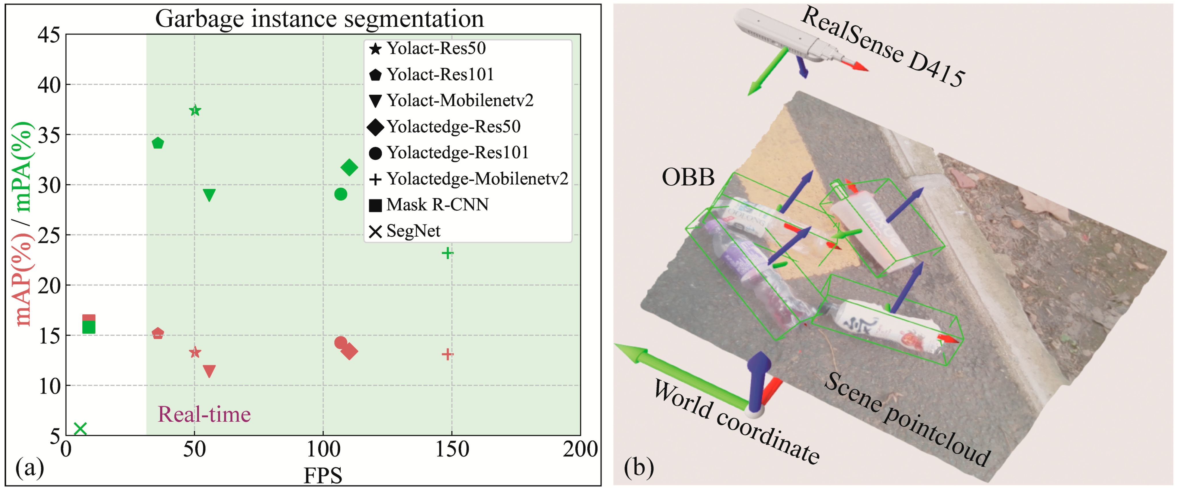
In order to improve the accuracy and efficiency of garbage detection and localization, this research focuses on detecting and calculating the spatial location of garbage instances under the scene point cloud reconstructed by the depth camera. Garbage detection is performed using the real-time instance segmentation model Yolactedge to obtain the garbage mask from RGB images. The point cloud of garbage instances is then segmented from the overall point cloud using the mask. As shown in Figure 1a, the TACO-28 [8] training Yolactedge families models, Mask R-CNN [4] and SegNet [9] achieved the highest mPA of 37.4% for mask under real-time detection, and also achieved a 10% mPA on the outdoor road garbage image data custom-collected with RealSenseD415, and then implemented point cloud segmentation of garbage instances. The assessed Oriented Bounding Boxes (OBB) is shown in Figure 1b.
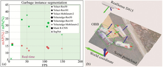
Figure 1.
(a) On the TACO-28, there is a trade-off between speed and performance for various instance segmentation approaches. Where bbox mAP and mask mPA are represented by red and green shapes, respectively. (b) The RealSenseD415 camera captured and reconstructed the scene point cloud at (0, 0, 750, 0, 135, 90) in the world coordinate system, and the OBB of the garbage instances calculated after point cloud segmentation and DBSCAN clustering.
In summary, the contributions are listed as follows: (1) a garbage dataset consisting of groups of RGB and depth images is created (2) a novel approach by combining a real-time instance segmentation model, a point cloud processing algorithm, and a vision-robot grasp system to straight-forwardly compute the pose of garbage in a clutter environment is introduced. we made the following works: (1) retraining Yolactedge using TACO-28, (2) segmenting and clustering garbage instance point cloud, (3) computing OBB, and (4) obtaining the robot grasp pose after hand-eye calibration. The paper’s structure is as follows: Section 1 provides an introduction and background information. Section 2 reviews the relevant literature. Section 3 describes the strategies employed for training instance segmentation models. Section 4 presents the obtained results. Finally, Section 5 provides the conclusions of the study.
2. Related Works
Object Detection. Object detection [10] usually employs one of two architectures: one-stage detection and two-stage detection. One-stage detectors, such as the YOLO [2,7] and SSD [11] families, are designed for real-time use while they reach a compromise in precision. They perform object detection by predicting both the classes and locations of objects in a single step using a regression problem approach [3], whereas two-stage detectors require two steps, the first of which finds class-agnostic region proposals and the second of which classifies them into class-specific output bboxes. Fast R-CNN [12] use the Selective Search algorithm [13] to select region proposals in the first stage, while Faster R-CNN [14] proposed a Region Proposal Network (RPN) integrated into Fast R-CNN to replace the Selective Search algorithm, and then have two branches to predict classes and bbox of object respectively in the second stage.
Sematic Segmentation. The goal of semantic segmentation, as described in FCN [15] and SegNet [9], is to predict the classes of each pixel in an image and the region of pixels with the same category is the predicted mask. Due to the dominance of fully connected layers in terms of model parameters, FCN and SegNet were specifically designed to utilize only the convolutional layer. which can accept any size image as input and output same size mask with efficient inference and learning. SegNet is used for scene interpretation tasks and sematic segmentation because of its high inference efficiency.
Instance Segmentation. Instance segmentation is related to yet distinct from sematic segmentation. While semantic segmentation aims to predict a segmentation mask for each pixel in an image, instance segmentation focuses on predicting a segmentation mask for each individual instance present in the image. On the other hand, object detection focuses on pre Mask R-CNN [4], two-stage detectors for instance segmentation that are employed feature pyramid network (FPN) [16] and region proposal network (RPN) [14]. By adding a mask prediction branch, Mask R-CNN became the leading model for instance segmentation and were successfully applied in various tasks, including the instance segmentation of garbage images in studies such as [3,5,8], where it demonstrated outstanding detection accuracy. However, the two-stage detector model has a complex structure thus requires more computational resources to achieve real-time detection, this makes it difficult to deploy the model especially on embedded platforms. The goal is to provide high frame rate object detection with guaranteed accuracy using single-stage detectors for real-time object detection, such as YOLO [2,7], SSD [11] serial models, and EfficientDet [17].
In order to build a single-stage structural model to solve the problem of a two-stage detector that relies heavily on feature localization, the Yolact [18,19] framework was introduced as a single-stage alternative. This framework employs two parallel branches: one generates a dictionary of non-local prototype masks, while the other predicts a set of linear combination coefficients for each instance. Finally, it is necessary to linearly combine the prototypes using the corresponding predicted coefficients and then crop with a predicted bounding box for each object. Yolact families [18,20] model can achieve 34.1% mAP on MS COCO [19] at 33.5 FPS, which is fairly close to the state-of-the-art approaches while still running at real-time. In [21], authors propose the first video-based Yolactedge architecture based on Yolact, which perform inference up to 30.8 FPS at a Jetson Xavier and 172.7 FPS on an RTX 2080Ti respectively. The performance migration of Yolactedge’s real-time instance segmentation to garbage segmentation is feasible and practical.
Waste dataset. Early CNN image classification algorithms were limited to categorize images, this leads to the labeling of certain garbage datasets such as TrashNet [22], Waste images, and Open Litter Map [23] with only the category of the garbage and its presence on a plain background. Extended TACO [8], Trash-ICRA19 [24], Drinking waste [22] are examples of datasets used for garbage target detection level, for labeling the class and bbox of all targets in the image against a complex background. However, the location of garbage class, without the precise edges of the garbage in the scene, is inconvenient for network to subsequent operations like grabbing or sucking. These issues may be solved if the masks of the garbage instances could be acquired. Therefore, the dataset used for garbage instance segmentation needs to be manually labelled with the class and mask of the garbage instance in the complex background, with the minimum enclosing box of the mask as the bbox of the instance. Table 1. lists some of the current publicly available datasets with instance masks, where Wade-AI [23], UAVVaste [6], MJU-Waste [25] and Cigarette butt tag all instances of trash in an image as a single object (rubbish or cigarette). TrashCan [26] dataset contain undersea trash, flora and fauna, with eight trash-related categories labelled. TACO [8], a consecutive growing free open dataset, contains 1500 high resolution images in diverse environment annotated with 4783 instances and divide them into 60 categories of litter which belong to 28 top classes. TACO offers a substantially more detailed range of garbage image scenes and annotated instances than the previous five datasets, making it more suitable to model learning and prediction of garbage instances in complicated contexts.

Table 1.
Publicly available garbage dataset for instance segmentation purpose.
There are several public garbage data sets, as shown in Table 1, that can be used for pre-training deep models, and the aforementioned associated research work [28,29], such as the instance segmentation model [18,19], provides the theoretical foundation and previous knowledge for garbage identification and segmentation. These models, data sets, and point cloud processing techniques can all be used together to quickly and accurately identify garbage objects in an outdoor environment.
3. Methodology
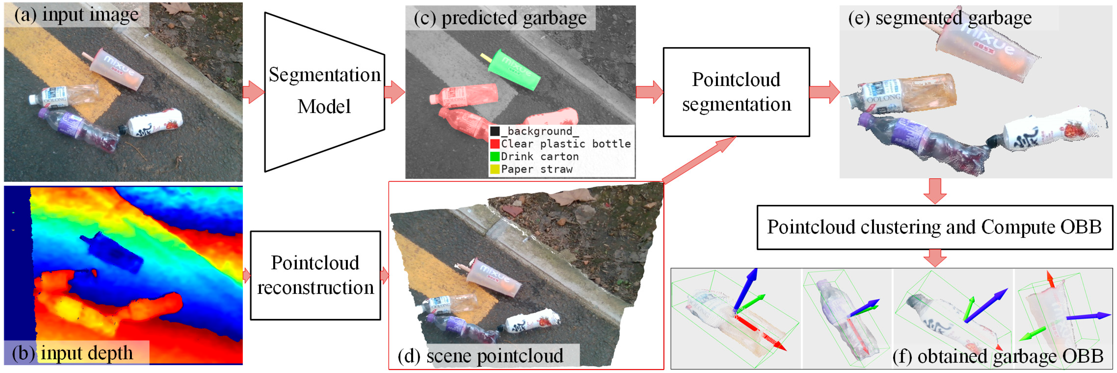
Using deep-learning-based instance segmentation and point cloud processing, this study proposed an architecture for garbage segmentation and 3D spatial localization. As shown in Figure 2, the input data consists of a pair of registered color and depth images captured by Intel’s RealSenseD415 camera. Firstly, the color image is fed into Segmentation Model N, which predicts the class and mask of each garbage instance in the image. This process can be expressed as , where N, Icolor, and respectively represent the DL model, RGB color image, and predicted C masks. Simultaneously, combine the camera intrinsic parameters (fx, fy, u0, v0) and depth image to create the entire scene point cloud by referring the Formula (1).
where is one of the point in the point cloud , Idepth is depth image, fx, fy, u0, v0 is camera intrinsic parameters and W, H is the width and height of RGB image respectively. In addition, the color of Pi is the RGB value at the (u + v × W) position in Icolor.

Figure 2.
The algorithm schematic for garbage object detection and 3D spatial localization in this research. The segmentation model N predicts garbage’s classes and masks, which are then used to split the garbage instances point cloud from the entire scene point cloud. Then, using the DBSCAN [30] clustering algorithm, remove the interference point and calculate the OBB for garbage.
Secondly, once we have achieved the , we can utilize it to extract the garbage point cloud from the entire scene point cloud using the Formula (2).
where is one of the C extracted garbage point cloud .
Finally, a point cloud clustering algorithm, based on DBSCAN [30], was adopted to fine-tune the splited . The main reason of this step is to remove outliers and calculate the best-fitting 3D OBB for .
Segmentation Models
Mask R-CNN. It is two-stage detectors that uses FPN [16] and RPN [14] for instance segmentation and achieves exceptional performance. Mask R-CNN [4] consists of three parts: (1) a shared convolutional layer as the “backbone” for feature extraction. (2) The RPN is used to generate a large number of candidate regions to be identified from the feature map, and (3) the network head, which contains 3 branches for category classification, bbox regression, and mask prediction. The combination of transfer learning and pre-trained backbone parameters allows for the efficient application of Mask R-CNN to new garbage instance segmentation tasks.
Yolact and YolactEdge. Pixels adjacent to each other in an image may belong to regions of the same instance, leading to spatial coherence in the corresponding masks. However, the spatial coherence can be lost when using fully connected layers, as they do not effectively preserve this information. As for one-stage detector, the fully connected layer is generally used as the output layer for classification and bbox regression. Two-stage detector, i.e., Mask R-CNN, uses ROI Align to preserve the spatial information of pixels, and the mask prediction branch in Network head also needs to use FCN [15]. However, doing so increases the time consumption significantly. To address this issue, Yolact [18] introduces two parallel networks called Protonet and Prediction Head. Protonet generates prototype masks, while Prediction Head predicts mask coefficients. These components are then combined using a linear combination to produce the final masks. In addition, in [20], authors introduced a Fast NMS, which significantly improves speed compared to conventional NMS. All of these new structures make Yolact a high-performance and state-of-the-art single-stage detector for instance segmentation. Yolactedge [21] applies two main strategies to further accelerate the speed-accuracy trade-off. Firstly, different precision levels are assigned to the components of the deep-learning model. Yolact’s backbone and FPN are converted to INT8 precision, while Protonet and Prediction Head are converted to FP16 precision, and ran them on Jetson AGX Xavier. The precision was tested on the MS COCO val2107 dataset [19], and the frame rate was improved by 21.3 with a slight reduction in mAP. Secondly, FeatFlowNet is introduced to transform previous key frames into current non-key frames. By applying a partial feature transform design, the computational costs associated with backbone’s convolutional layers are avoided, leading to additional speed improvements. Given that the Yolactedge families models achieve frame rates of up to 172 FPS and mAP values of 34.1% on MS COCO, their application to garbage instance segmentation in this study is highly practicable.
SegNet. SegNet [9] is a deep convolutional encoder-decoder framework with a high level of detail for image sematic segmentation. The encoder-decoder structure has a total of 11 blocks. In the encoder part, SegNet can utilize the convolutional layers of VGG16 [31]. It consists of 5 convolutional blocks, each comprising 2 or 3 convolutional layers followed by a max pooling layer. The max pooling layer retains the index of the maximum feature value in a sparse matrix, preserving the position information for subsequent up sampling operations in the decoder. Accordingly, the decoder has 5 blocks corresponding to the encoder, each with an up sampling layer and 2 or 3 convolutional layers. After the output layer of the decoder is the SoftMax layer. The principle is that the features in the image are first extracted by the encoder to obtain a low resolution highly aggregated feature map, which is then mapped by the decoder to a feature map of the same resolution size as the model input layer by using the index of the max pooling in the encoder, called up sampling. Batch Normalization layers are attached to each convolutional layer in the decoder to speed up the convergence of the training process and to make the training data more evenly distributed and fixed in the sample space. After 4 up sampling operations, the size of the feature map becomes the same as the input image size, and then the SoftMax layer converts the feature values in the feature map into probabilities, thus achieving multi-classification of pixel values.
4. Experiments and Results
In this section, we introduce the configuration and training details of Yolact, Yolactedge, Mask R-CNN, and SegNet, and then describe the processing steps of the dataset in order to train each model. The hardware environment of these models uses an Intel i9 CPU, an NVIDIA GeForce GTX 2080Ti GPU, and 32 GB of running memory, a powerful computing platform to provide strong support for model training and inference. The optimal configuration of the model parameters was summarized through analysis of the model’s training and testing results.
4.1. Implementation Details
Dataset processing. The TACO dataset currently contains 1500 high-definition rubbish images taken with mobile phones, each with instance segmentation information saved as a json file in COCO format, and randomly divided into training, test, and validation sets in the proportion of 80%, 15%, and 5%, respectively. Due to limited computing resources (an RTX 2080Ti GPU with 11 GB video memory), the input images needed to be scaled to dimensions of either 550 × 550 × 3 or 512 × 512 × 3, and since TACO has 60 categories (28 super categories), the code will apply a large amount of memory space when generating the training data. Therefore, it is necessary to keep the aspect-ratio scaling for the 1500 high-resolution images in TACO. Specifically, the width of all images was scaled to 640, the height was scaled by a ratio, and the instance labels in the image segmentation points and bounding boxes (x, y, w, h) were also scaled accordingly, with the json file being updated accordingly. On the other hand, this paper only classifies the garbage according to the 28 super categories defined by TACO, so we also need to process the defined categories in the json file as 28 super categories, and change the category id number of each instance so that it maps to the corresponding category. After doing these processes, this study named the dataset TACO-28. Finally, a software application was developed using the Intel RealSense SDK to capture real-time RGB and Depth streams of rubbish in various environments. The depth stream data was used to reconstruct the scene point cloud and calculate the OBB of the rubbish instances. The garbage instances in the RGB images were then manually labelled to test the accuracy of the segmentation model.
Training details. The transfer learning scheme is applied to the fast training and optimization of the model. For the Yolactedge models, we conducted experiments using different backbones, including Res50, Res101 [32], and MobileNetV2 [33]. To initialize the model weights, we utilized the pretrained model parameters from ImageNet. and we fine-tuned these weights using the TACO [8] dataset based on the open source code of Haotian Liu [21]. Learning-rate, momentum, decay and iteration are set to 0.003, 0.9, 0.0005, 80,000 respectively. For Mask R-CNN and SegNet, backbone uses VGG16 and its weights are initialized with ImageNet-pretrained weights.
Model evaluation metrics. The evaluation of the instance segmentation model includes metrics for object detection precision, mask segmentation precision, as well as real-time performance and parametric quantities. The positioning precision of the model for each category is represented by the APi value, while the positioning accuracy for all categories in the dataset is represented by the mAP = sum(APi)/n value. Comparatively, the mask segmentation precision of the instance segmentation model is evaluated by mIoU, mAP, PA, etc. Since the TACO dataset contains 60 categories, some of which have insignificant feature differences or a small number of instances, it can be challenging for the instance segmentation model to achieve high precision in category detection, resulting in low values for the calculated evaluation metrics, and this is why we used TACO-28. In this study, the main purpose is the inference speed of the model and the accuracy of the mask segmentation. The higher the accuracy of the mask, the more accurate the segmented point cloud will be, which will simplify the computation of the point cloud OBB. Therefore, the main evaluation metrics used in this study are mPA (mean Pixel Accuracy) and frame rate, as they provide insights into the accuracy and speed of the model’s performance.
4.2. Model Training and Testing Results
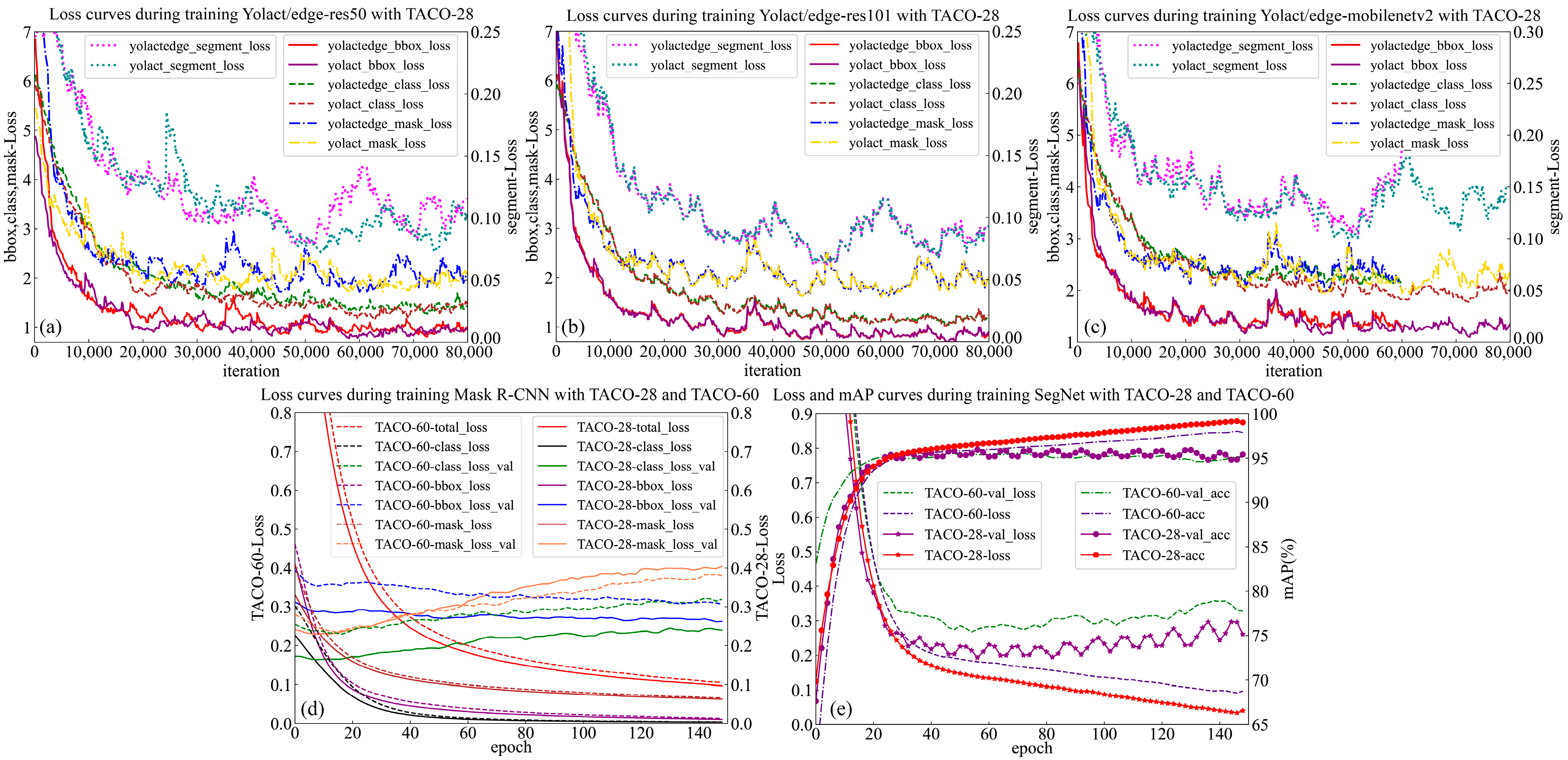
Training result. As shown in Figure 3a–c, after 80,000 iterations (533 epochs), the class, bbox, and mask loss of both Yolact and Yolactedge start off significantly lower until it plateaus at around 1. Firstly, comparing Yolact and Yolactedge, as Haotian Liu [21] said, the latter’s mask mAP falls behind the former. In Figure 3a,c, it can be observed that the individual loss values of Yolact are smaller than those of Yolactedge, but the difference is small and the trend is basically the same. In particular, in Figure 3b, the loss curves of the two models are almost identical. By comparing the loss curves for different backbones, it is noted that the loss curve for Mobilenetv2 is higher than that for Res50, and the loss curve for Res50 is higher than that for Res101. This suggests that increasing the depth of the backbone and the number of parameters improves the model’s accuracy in terms of loss values. Finally, despite the models and backbones, the loss of bbox is lower than that of class, and the loss of class is lower than that of mask, implying that Yolact families object detection is better than mask segmentation. Meanwhile, in this study, Mask R-CNN and SegNet were also trained with TACO-28 and TACO-60 in turn. As shown in Figure 3d,e, the loss values of Mask R-CNN and SegNet tended to be smooth after 150 epochs of training, the loss value of TACO-28 is lower than that of TACO-60, indicating that the more categories the dataset is divided into, the more difficult it is for the model to distinguish the garbage categories. It is important to note that the true performance of the models cannot be solely summarized based on training loss data. Various metrics will be used to evaluate and characterize the performance of each model.
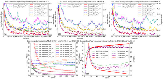
Figure 3.
Loss curves during training of these models with TACO-28. (a–c) show the loss curves for each branch of Yolactedge after training 80,000 iterations with Res50, Res101, and Mobilenetv2, respectively. (d,e) are the loss curves of Mask R-CNN and SegNet after training for 150 epochs, respectively.
Testing result. The AP value is used to characterize the precision of the Yolactedge and Mask R-CNN models’ garbage target localization, while the same precision evaluation metrics as SegNet are used in this study for their mask output, i.e., mIoU, mPA, and PA. As shown in Table 2, Mask R-CNN and SegNet have the highest number of parameters and the lowest FPS due to their complex network structures, which makes fine-tuning with limited datasets extremely challenging. The TACO dataset contains images with diverse backgrounds, consisting of 60 categories (28 super categories) and numerous small target instances. However, SegNet, being a semantic segmentation network, struggles with distinguishing the pixel categories of multi-category small targets, leading to significantly low evaluation metrics for mask segmentation on the test set. Mask R-CNN, as a Faster R-CNN inherited from two-stage, achieved a mAP of 16.43 for the localization of garbage instances after 150 epochs of training on TACO-28, which is the best performance among the models applied in this study and is close to the mAP value of 17.6 ± 1.6% obtained in TACO [8] after training Mask R-CNN with TACO-10. However, the accuracy of the output mask still lags behind that of the Yolactedge models. Due to the simple scaling method used in processing the dataset, many features of small objects are lost, resulting in even lower detected mAP values compared to those in TACO.
Table 2.
Comparison each model’s performance in TACO-28. The PA values in Table 2 are above 94% because the model correctly classifies a large proportion of the background pixels.
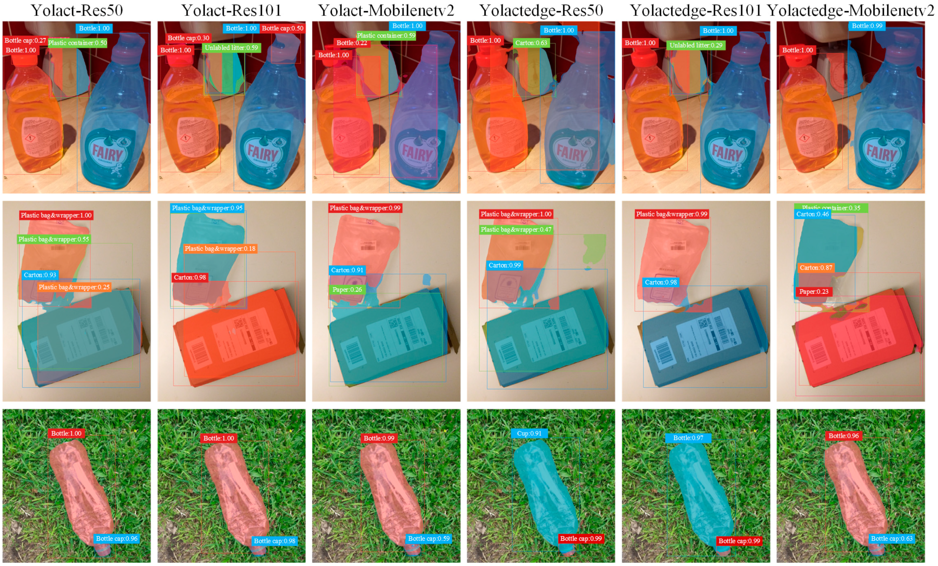
The values of mIoU, mPA and PA are shown in Table 2. For Yolactedge families, comparing Mobilenetv2 and Res101, Res50 gives optimal values of mIoU and mPA of 25.03% and 37.40%, respectively. This indicates that as the backbone becomes lighter, prediction accuracy decreases while the model’s real-time performance improves, as shown in columns 3 and 6 of Figure 4.
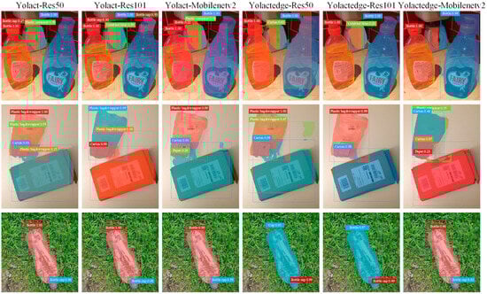
Figure 4.
Comparison mask segmentation results for each model. All of these models can detect garbage instances from images, but there are cases of misclassification and inaccurate mask segmentation. Firstly, lightweight Mobilenetv2 has the lowest mask segmentation accuracy. When comparing the prediction results of Yolact and Yolactedge, the mIoU and mPA of the predicted masks decrease by about 2% and 5%, respectively, after converting the model component to TensorRT, although the frame rate increases.
Yolactedge achieves a near 2× speedup by converting the modules in Yolact to TensorRT, as shown in Table 2, with the frame rate increasing from 35.76 to 110.16 for Res101However, there is a slight 2% decrease in both localization precision and mask segmentation precision. As shown in Figure 1a, Yolactedge-Res50/Res101 can reach 100 FPS with 30% mPA accuracy, which is suitable for high-speed and high-accuracy detection tasks.
4.3. Garbage Point Cloud Extraction
After achieving the fine-tuned weight parameters, we can deploy the garbage instance segmentation model to extract garbage masks from images or videos in real-time. For each pair of registered RGB and depth frames, we can start by reconstructing the scene’s point cloud. Then, by utilizing the masks generated by the model, we can extract the point cloud corresponding to each garbage instance. Finally, compute OBB for each instance by referring to DBSCAN [30] and the OBB algorithm. Due to the obvious directional characteristics of the RealSense’s collected point cloud, only the visible side of the point cloud can be measured, and many distant and close interfering points are generated at the object’s edge. To remove interfering points, point cloud filtering, clustering, and segmentation algorithms can be used. The DBSCAN-based point cloud clustering method is used in this paper, without the user setting the number of clusters a priori, clusters with complex shapes can be divided, and points that do not belong to any cluster can be found. Dense data sets of arbitrary shape can be clustered, and clustering algorithms such as K-Means are generally only suitable for convex data sets [34].
The DBSCAN algorithm requires two input parameters, ε and μ (representing the minimum points), which determine the clustering degree of the point cloud. Since there are no standard point clouds for garbage instances, it is challenging to determine the similarity between the segmented point clouds and the true value clouds. Therefore, in this study, we aimed to determine the optimal values for these two parameters. To achieve this, we followed a two-step process. First, we selected images and point clouds from three different scenes and segmented the point clouds using the predicted masks from Yolactedge. Secondly, the point clouds of garbage instances in each of the three scenarios were then clustered using the parameters ε = (2, 2.5, 3, 3.5, 4, 4.5, 5) and μ = (10, 20, 30, 40, 50). The clusters were sorted in descending order by the number of points and then the first cluster was taken as the point cloud of the garbage instance with the interfering points removed. The percentage of interfering points removed was also calculated.
The removal rates of interfering points were compared and visualized in a bar chart, as shown in Figure 5. After sorting the 35 rates, the parameter pairs of ε and μ corresponding to the middle 4 values were selected as pre-selection parameters. Figure 6 shows a visualization of the results of point cloud removal for three scenes with various parameter pairs, where the points in blue are the removed points.
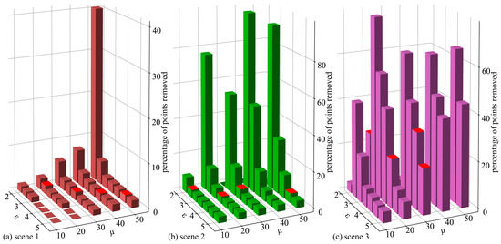
Figure 5.
The removal rate (number of points removed/total number of points) of the rubbish instance point cloud is based on the DBSCAN clustering algorithm. Where ε = (2, 2.5, 3, 3.5, 4, 4.5, 5), μ = (10, 20, 30, 40, 50). Whereas the red bin denotes the 4 values in the middle of the 35 removal rates sorted. (a) scene 1, (b) scene 2, (c) scene 3.
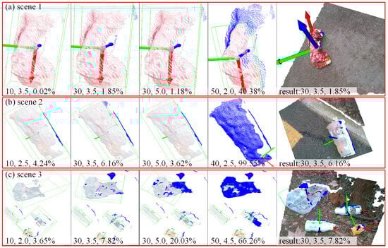
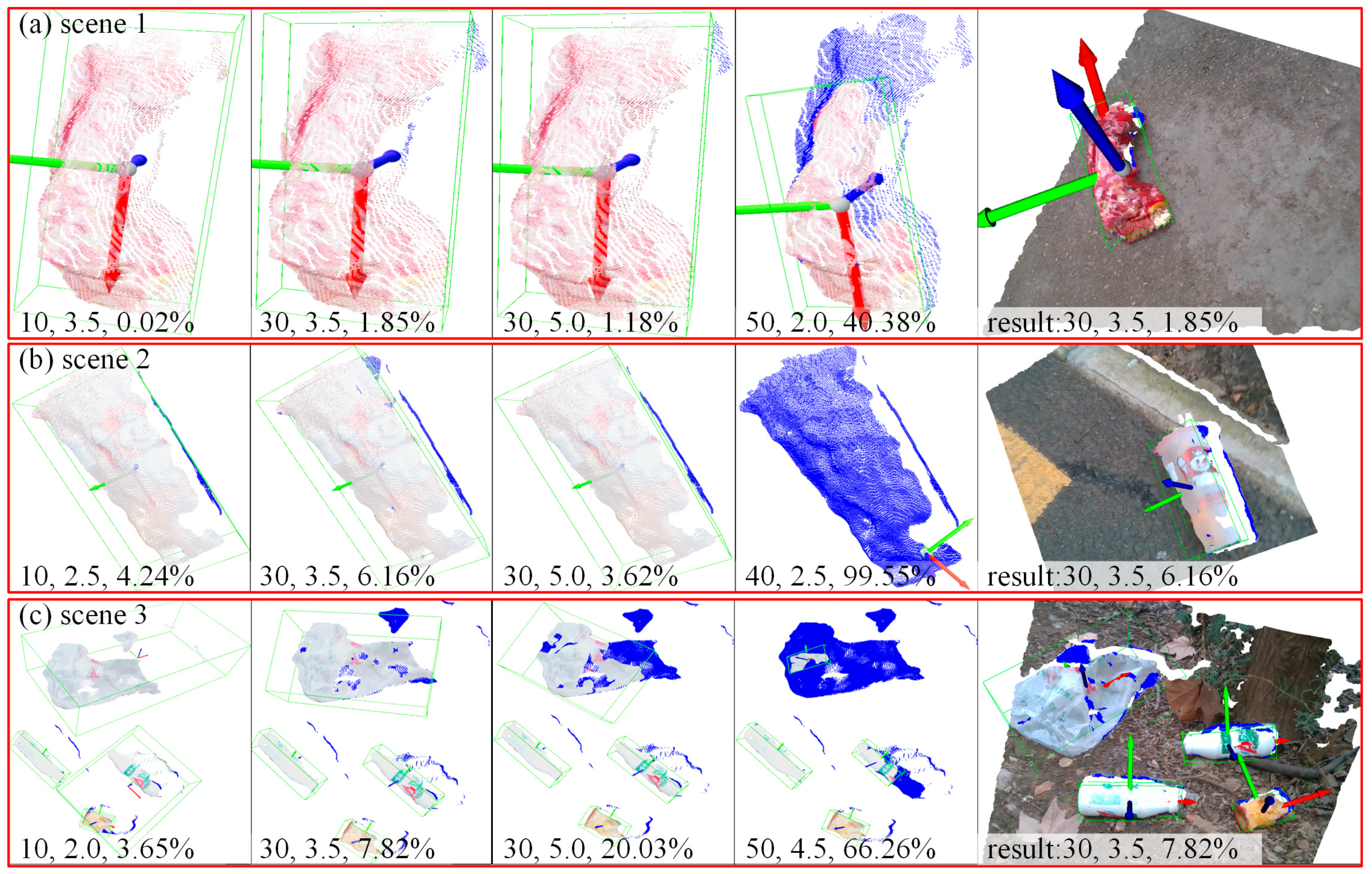
Figure 6.
A visual comparison of the interfering point removal rates and results for the corresponding 3 scenes in Figure 5. The last column shows the 3 scene point clouds with the interfering points (blue points) removed and the calculated OBB for ε and μ of 3.5 and 30, respectively. The numbers at the bottom of each subplot indicate μ, ε and point removal rate in that order.
The number of points and point spacing of the captured garbage instance point cloud vary due to differences in camera position, viewing direction, and scene and garbage instance size when capturing RGB and point cloud. Consequently, a set of ε and μ parameters may completely remove the garbage instance point cloud in some scenes, as depicted in column 4 of Figure 6. Conversely, in other scenes, such as column 1 of Figure 6c, the parameter combination may hardly remove any interfering points, so that the calculated OBB will not fit perfectly in all scenes. As shown in column 1 of Figure 6c, causing the calculated OBB will deviate significantly from the actual size and location of the garbage instances, so that a set of parameter combinations cannot be perfectly adapted to all scenarios.
In this study, by referring to the interfering point removal rate and visualization results in these three scenes. It was observed that when ε and μ were set to 3.5 and 30, respectively, the interfering point removal rate was in the middle. From Figure 6, it can be observed that at current setting, the interfering point removal rate was less than 10%, and the calculated OBB precisely encapsulated the garbage instances in terms of size and location. Therefore, this paper selects ε and μ as 3.5 and 30, respectively, as the final combination of point cloud clustering parameters.
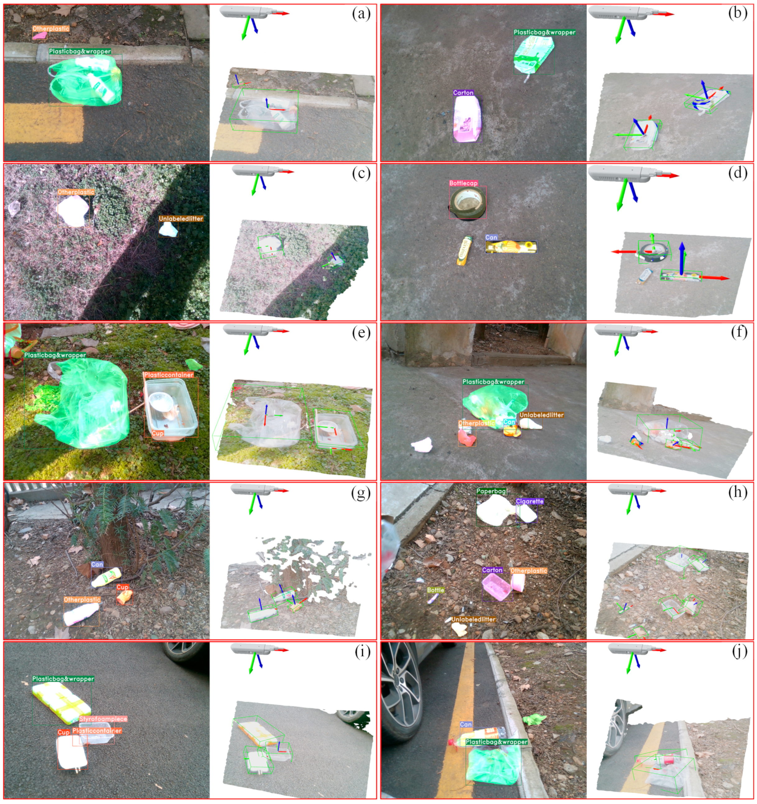
Up to this point, we have trained the Yolactedge model, determined key parameters for point cloud clustering, and performed post-processing and visualization of the Yolactedge prediction results and point cloud data using OpenCV and Open3D, as shown in Figure 7. To verify the generalization performance of the Yolactedge model and the representativeness of the TACO dataset, we fed custom-collected outdoor garbage images to the Yolactedge model for mask prediction, and the results are shown in the left image of each subplot of Figure 7. Thanks to the wide range of scenes included in the TACO-28 dataset, the Yolactedge model trained on it can be used directly to predict the categories and masks of garbage in the custom-collected dataset, thus reducing the need for a lot of tedious data annotation and enabling the identification of garbage on our own collected dataset. However, due to the overlapping characteristics of different garbage categories in the TACO dataset, the prediction accuracy of the Yolactedge model for garbage classification is affected, leading to specific category errors in the identified garbage shown in the images of Figure 7. Since the calculation of the evaluation metrics for localization and segmentation accuracy relies first and foremost on the class correctness, low class accuracy leads to a failure to improve their accuracy values, and it is known from [8] that the authors also designed three different class_score methods with the intention of improving localization accuracy, but the highest AP accuracy obtained by the fine-tuned Mask R-CNN model on TACO-10 is still only 20%.
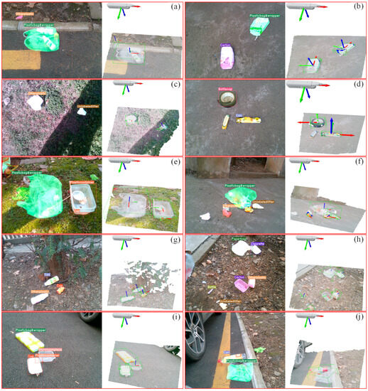
Figure 7.
The results of the garbage detection and 3D spatial localization algorithms proposed in this study are shown. Each subplot in (a–j) depicts the classes and masks of garbage instances predicted by the Yolactedge-res101 model on custom-collected outdoor rubbish data (left image), as well as the reconstructed entire scene point cloud, segmented rubbish instance point cloud, and computed OBB (right image).
In addition, the accuracy of mask segmentation is the subject of this research. The segmented instance point cloud with a high quality mask has the fewest interfering points, which helps to improve the accuracy of the calculated OBB. Since the TACO dataset solely consists of garbage images without associated point clouds, the only viable option for obtaining garbage instance point clouds is by utilizing the paired images and point clouds from the custom-collected dataset. The scene point cloud acquired by the camera is shown on the right image of each subplot of Figure 7, and also shows the splited point cloud of garbage instances by using its associated predicted mask. The accuracy of the predicted garbage’s 3D spatial position relies on two factors: firstly, the accuracy of the point cloud reconstruction by the RealSense D415 camera (with a Z-directional accuracy of less than 2%), and secondly, the subsequent calculations performed with the assistance of third-party equipment, such as robot arms for gripping, indirectly affecting the accuracy.
Vision-driven robotic grasp requires obtaining the garbage location and posture from a noisy, complex background scene image. In this work, deep learning networks like the Yolactedge model are then used for object recognition and segmentation. As we know, Robotic grasp is a challenging question that includes perception, planning, and control theory. Thus, research on the 3D reconstruction and measurement of objects helps with feature extraction or obtaining valuable information from RGB or point cloud data, which will then be used to grasp pose prediction. A typical vision-guided industrial robot system is shown as Figure 8.
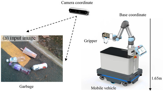
Figure 8.
Our vision-guided robotic grasp equipment for garbage picking up application.
The robot grasp system consists of mobile vehicle, UR robot, stereo camera and clamping tool. As can be seen from Figure 8, a RealSense D415 (product of Intel company) camera is mounted on the tool of UR5 robot, a two driving-links of gripping jaw is employed to pick up garbage through object detection and localization algorithm. Hand-eye coordination calibration technology is performed to establish the mathematic relationship between camera coordinate and robot base coordinate. The internal and external parameters of the robot grasp system is calibrated as:
Thus, the garbage grasp pose in Figure 7 is converted through intrinsic and extrinsic matrix from camera coordinate to robot base coordinate, some examples are shown in Figure 9.
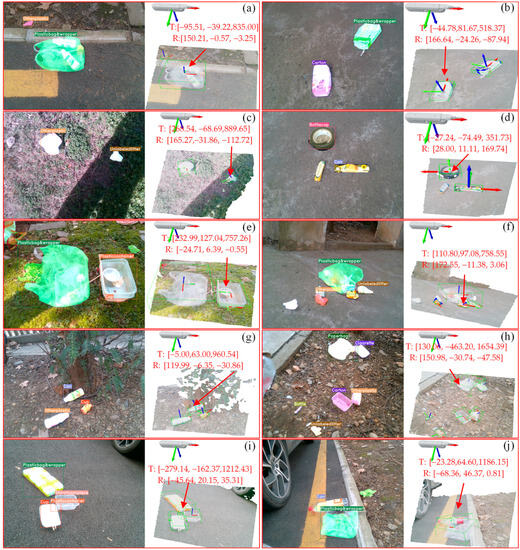
Figure 9.
Each subplot in (a–j) depicts the robot grasp pose calculating from camera coordinate to robot base coordinate (Translation and Rotation).
5. Conclusions
This research proposes an algorithmic architecture for improving the precision of garbage classification and localization by integrating computer vision and machine learning techniques. The proposed approach leverages RGB-D data captured by the RealSenseD415 camera and employs the Yolactedge model to predict the garbage class and mask from RGB images. By utilizing the predicted mask, the algorithm effectively separates the garbage instances’ point cloud from the overall scene point cloud. The spatial position and orientation of the garbage instances are determined by computing the OBB of the segmented point cloud using the DBSCAN clustering method, which eliminates interfering points and provides valuable information for robotic grasp applications. To facilitate the training process, the TACO dataset is pre-processed, and a custom-collected garbage dataset is generated. While the TACO dataset only consists of garbage image data, the fine-tuned Yolactedge model proves to be useful for garbage mask segmentation in the custom dataset, enabling the segmentation of point clouds and the calculation of garbage instance OBBs. This approach significantly reduces the laborious task of data annotation. The results indicate that the proposed approach can run at a maximum speed of 150 FPS and maximum mPA of 37%. Experimental evaluations on custom-collected datasets demonstrate the effectiveness of the proposed approach in achieving accurate garbage detection and spatial localization. The results highlight the potential of the algorithmic architecture in revolutionizing waste management processes, enabling intelligent garbage sorting, and facilitating robotic grasp applications.
Future work involves redefining garbage categories based on recycling standards to optimize detection performance and exploring the integration of 3D spatial localization with mobile robot garbage pickup or conveyor belt sorting systems. In summary, this research highlights the application of computer vision, machine learning, and intelligent image processing in garbage detection and localization, with implications for improving waste management and recycling processes.
Author Contributions
Conceptualization, Z.L.; Methodology, Z.L.; Software, T.C.; Formal analysis, T.C.; Writing—original draft, Z.L. and T.C.; Writing—review & editing, Z.C. (Zhenhua Cai) and Z.C. (Ziyang Chen). All authors have read and agreed to the published version of the manuscript.
Funding
This research received no external funding.
Institutional Review Board Statement
Not applicable.
Informed Consent Statement
Not applicable.
Data Availability Statement
The data presented in this study are available on request from the corresponding author. The data are not publicly available due to privacy.
Conflicts of Interest
The authors declare no conflict of interest.
References
- Carolis, B.D.; Ladogana, F.; Macchiarulo, N. YOLO TrashNet: Garbage Detection in Video Streams; IEEE: Piscataway, NJ, USA, 2020; pp. 1–7. [Google Scholar]
- Redmon, J.; Farhadi, A. Yolov3: An incremental improvement. arXiv 2018, arXiv:1804.02767. [Google Scholar]
- Jaikumar, P.; Vandaele, R.; Ojha, V. Transfer Learning for Instance Segmentation of Waste Bottles Using Mask R-CNN Algorithm; Piuri, V., Gandhi, N., Siarry, P., Kaklauskas, A., Madureira, A., Eds.; Springer International Publishing: Cham, Switzerland, 2021; pp. 140–149. [Google Scholar]
- He, K.; Gkioxari, G.; Dollár, P.; Girshick, R. Mask R-CNN. In Proceedings of the 2017 IEEE Conference on Computer Vision and Pattern Recognition, Honolulu, HI, USA, 21–26 July 2017. [Google Scholar]
- Majchrowska, S. Waste detection in pomerania: Non-profit project for detecting waste in environment. arXiv 2021, arXiv:2105.06808. [Google Scholar]
- Kraft, M.; Piechocki, M.; Ptak, B.; Walas, K. Autonomous, Onboard Vision-Based Trash and Litter Detection in Low Altitude Aerial Images Collected by an Unmanned Aerial Vehicle. Remote Sens. 2021, 13, 965. [Google Scholar] [CrossRef]
- Bochkovskiy, A.; Wang, C.-Y.; Liao, H.-Y.M. YOLOv4: Optimal Speed and Accuracy of Object Detection. In Proceedings of the 2020 IEEE Computer Vision and Pattern Recognition, Seattle, WA, USA, 13–19 June 2020. [Google Scholar]
- Proença, P.F.; Simões, P. TACO: Trash Annotations in Context for Litter Detection. arXiv 2020, arXiv:2003.06975. [Google Scholar]
- Badrinarayanan, V.; Kendall, A.; Cipolla, R. SegNet: A Deep Convolutional Encoder-Decoder Architecture for Image Segmentation. IEEE Trans. Pattern Anal. Mach. Intell. 2017, 39, 2481–2495. [Google Scholar] [CrossRef] [PubMed]
- Zou, Z.; Shi, Z.; Guo, Y.; Ye, J. Object detection in 20 years: A survey. arXiv 2019, arXiv:1905.05055. [Google Scholar] [CrossRef]
- Liu, W.; Anguelov, D.; Erhan, D.; Szegedy, C.; Reed, S.; Fu, C.-Y.; Berg, A. SSD: Single Shot MultiBox Detector. In Proceedings of the 2015 IEEE Conference on Computer Vision and Pattern Recognition, Boston, MA, USA, 7–12 June 2015; pp. 21–37. [Google Scholar]
- Girshick, R. Fast r-cnn. In Proceedings of the 2015 IEEE Conference on Computer Vision and Pattern Recognition, Boston, MA, USA, 7–12 June 2015. [Google Scholar]
- Uijlings, J.R.R.; van de Sande, K.E.A.; Gevers, T.; Smeulders, A.W.M. Selective Search for Object Recognition. Int. J. Comput. Vis. 2013, 104, 154–171. [Google Scholar] [CrossRef]
- Ren, S.; He, K.; Girshick, R.; Sun, J. Faster R-CNN: Towards Real-Time Object Detection with Region Proposal Networks. In Proceedings of the 2015 IEEE Conference on Computer Vision and Pattern Recognition, Boston, MA, USA, 7–12 June 2015; pp. 1–10. [Google Scholar]
- Long, J.; Shelhamer, E.; Darrell, T. Fully Convolutional Networks for Semantic Segmentation. In Proceedings of the 2014 IEEE Conference on Computer Vision and Pattern Recognition, Columbus, OH, USA, 23–28 June 2014; pp. 3431–3440. [Google Scholar]
- Lin, T.-Y.; Dollar, P.; Girshick, R.; He, K.; Hariharan, B.; Belongie, S. Feature Pyramid Networks for Object Detection. In Proceedings of the 2017 IEEE Conference on Computer Vision and Pattern Recognition, Honolulu, HI, USA, 21–26 July 2017; pp. 936–944. [Google Scholar]
- Tan, M.; Pang, R.; Le, Q.V. Efficientdet: Scalable and efficient object detection. In Proceedings of the IEEE/CVF Conference on Computer Vision and Pattern Recognition, Seattle, WA, USA, 13–19 June 2020; pp. 10781–10790. [Google Scholar]
- Bolya, D.; Zhou, C.; Xiao, F.; Yong, J.L. YOLACT++: Better Real-time Instance Segmentation. IEEE Trans. Pattern Anal. Mach. Intell. 2020, 44, 1108–1121. [Google Scholar] [CrossRef] [PubMed]
- Lin, T.-Y.; Maire, M.; Belongie, S.; Hays, J.; Perona, P.; Ramanan, D.; Dollár, P.; Zitnick, C.L. Microsoft COCO: Common Objects in Context; Pajdla, T., Schiele, B., Tuytelaars, T., Eds.; Springer International Publishing: Cham, Switzerland, 2014; pp. 740–755. [Google Scholar]
- Bolya, D.; Zhou, C.; Xiao, F.; Lee, Y.J. Yolact: Real-time instance segmentation. In Proceedings of the IEEE/CVF International Conference on Computer Vision, Long Beach, CA, USA, 15–20 June 2019; pp. 9157–9166. [Google Scholar]
- Liu, H.; Soto, R.A.R.; Xiao, F.; Lee, Y.J. Yolactedge: Real-time instance segmentation on the edge. In Proceedings of the 2021 IEEE International Conference on Robotics and Automation (ICRA), Xi’an, China, 30 May–5 June 2021; pp. 9579–9585. [Google Scholar]
- Serezhkin, A. Drinking Waste Classification. Available online: https://www.kaggle.com/arkadiyhacks/drinking-waste-classification (accessed on 4 September 2023).
- Foundation, L.S.D.I. Wade-ai. Available online: https://github.com/letsdoitworld/wade-ai (accessed on 4 September 2023).
- Fulton, M.; Hong, J.; Jahidul Islam, M.; Sattar, J. Robotic Detection of Marine Litter Using Deep Visual Detection Models. In Proceedings of the 2019 International Conference on Robotics and Automation (ICRA), Guangzhou China, 26–28 June 2019; pp. 5752–5758. [Google Scholar]
- Wang, T.; Cai, Y.; Liang, L.; Ye, D. A Multi-Level Approach to Waste Object Segmentation. Sensors 2020, 20, 3816. [Google Scholar] [CrossRef] [PubMed]
- Hong, J.; Fulton, M.; Sattar, J. TrashCan: A Semantically-Segmented Dataset towards Visual Detection of Marine Debris. arXiv 2020, arXiv:2007.08097. [Google Scholar]
- Bashkirova, D.; Abdelfattah, M.; Zhu, Z.; Akl, J.; Alladkani, F.; Hu, P.; Ablavsky, V.; Calli, B.; Bargal, S.A.; Saenko, K. ZeroWaste Dataset: Towards Deformable Object Segmentation in Extreme Clutter. arXiv 2021, arXiv:2106.02740. [Google Scholar]
- Liao, J.; Luo, X.; Cao, L.; Li, W.; Feng, X.; Li, J.; Yuan, F. Road garbage segmentation and cleanliness assessment based on semantic segmentation network for cleaning vehicles. IEEE Trans. Veh. Technol. 2021, 70, 8578–8589. [Google Scholar] [CrossRef]
- Vivekanandan, M.; Jesuda, T. Deep Learning Implemented Visualizing City Cleanliness Level by Garbage Detection. Intell. Autom. Soft Comput. 2023, 36, 1639–1652. [Google Scholar] [CrossRef]
- Ester, M.; Kriegel, H.-P.; Sander, J.R.; Xu, X. A density-based algorithm for discovering clusters in large spatial databases with noise. In Proceedings of the Second International Conference on Knowledge Discovery and Data Mining, Portland, OR, USA, 2–4 August 1996; pp. 226–231. [Google Scholar]
- Simonyan, K.; Zisserman, A. Very Deep Convolutional Networks for Large-Scale Image Recognition, Computer Vision and Pattern Recognition. arXiv 2014, arXiv:1409.1556v6. [Google Scholar]
- Khan, A.; Wahab, N. Deep Residual Learning for Image Recognition. In Proceedings of the 2015 IEEE Conference on Computer Vision and Pattern Recognition, Boston, MA, USA, 7–12 June 2015; IEEE Computer Society: Los Alamitos, CA, UUSA, 2015. [Google Scholar]
- Sandler, M.; Howard, A.; Zhu, M.; Zhmoginov, A.; Chen, L.-C. Mobilenetv2: Inverted residuals and linear bottlenecks. 2018; pp. 4510-4520. [Google Scholar]
- Guo, Z.; Liu, H.; Pang, L.; Fang, L.; Dou, W. DBSCAN-based point cloud extraction for Tomographic synthetic aperture radar (TomoSAR) three-dimensional (3D) building reconstruction. Int. J. Remote Sens. 2021, 42, 2327–2349. [Google Scholar] [CrossRef]


Disclaimer/Publisher’s Note: The statements, opinions and data contained in all publications are solely those of the individual author(s) and contributor(s) and not of MDPI and/or the editor(s). MDPI and/or the editor(s) disclaim responsibility for any injury to people or property resulting from any ideas, methods, instructions or products referred to in the content. |
© 2023 by the authors. Licensee MDPI, Basel, Switzerland. This article is an open access article distributed under the terms and conditions of the Creative Commons Attribution (CC BY) license (https://creativecommons.org/licenses/by/4.0/).