Abstract
In data science and visualization, dimensionality reduction techniques have been extensively employed for exploring large datasets. These techniques involve the transformation of high-dimensional data into reduced versions, typically in 2D, with the aim of preserving significant properties from the original data. Many dimensionality reduction algorithms exist, and nonlinear approaches such as the t-SNE (t-Distributed Stochastic Neighbor Embedding) and UMAP (Uniform Manifold Approximation and Projection) have gained popularity in the field of information visualization. In this paper, we introduce a simple yet powerful manipulation for vector datasets that modifies their values based on weight frequencies. This technique significantly improves the results of the dimensionality reduction algorithms across various scenarios. To demonstrate the efficacy of our methodology, we conduct an analysis on a collection of well-known labeled datasets. The results demonstrate improved clustering performance when attempting to classify the data in the reduced space. Our proposal presents a comprehensive and adaptable approach to enhance the outcomes of dimensionality reduction for visual data exploration.
1. Introduction
1.1. Motivation
Dimensionality reduction (DR) techniques are essential tools in data science, enabling the transformation of high-dimensional data into lower-dimensional representations, often in 2D or 3D. These techniques have experienced a significant increase in popularity across various fields, including machine learning, visualization, and experimental domains [1,2,3]. The widespread adoption of DR techniques is attributed to the prevalence of high-dimensional datasets, and their reduction to lower dimensions can facilitate tasks such as classification and visualization [4]. DR algorithms are very useful for data visualization because they can help users to obtain a sense of the distribution of the high-dimensional data, such as the graph, the neighborhoods, or their global structure [1]. There are two primary families of DR algorithms: linear and nonlinear [5,6]. The popularity of these techniques is evident from the substantial number of recent surveys dedicated to exploring these algorithms [5,7,8,9,10].
However, the performance of different DR algorithms can vary significantly, making it challenging to select the most appropriate one for a specific task [11]. The results of the DR algorithms can lead to misinterpretations, resulting in researchers recognizing clusters or patterns that are not actually present, as demonstrated by Huang et al. in their work [12]. Furthermore, not all labeled models achieve perfect separation when using DR results, and many models may require hyperparameter fine-tuning to obtain satisfactory outcomes. For instance, t-Distributed Stochastic Neighbor Embedding (t-SNE) [13], a widely used algorithm, is heavily reliant on the fine-tuning of hyperparameters. Identifying optimal values can be challenging, as we often lack an understanding of the structure of high-dimensional data [14].
1.2. Related Work
In the field of information visualization, dimensionality reduction serves as a common and valuable tool for exploring high-dimensional data. Many visualization systems leverage dimensionality reduction techniques to gain insights into complex datasets. For instance, in the exploration of document sets, techniques like UMAP (Uniform Manifold Approximation and Projection) projection of doc2vec embeddings from scientific documents have been used to build interactive tools [15,16,17]. Silva and Bacao also developed an interactive tool called MapIntel, which utilizes BERT embeddings and UMAP for document exploration [18,19].
Moreover, dimensionality reduction techniques can aid in the exploration of highly structured documents, such as medical records [20]. By applying DR to such datasets, researchers and practitioners can gain valuable insights and navigate through the complexities of the data, facilitating more effective analysis and understanding. However, as shown by Wattenberg et al. [14], the clusters that may appear after the projection are largely dependent on the hyperparameter specification. But if the distribution is unknown, it may not be possible to find the proper values for those.
Indeed, dimensionality reduction techniques are widely employed by researchers to compare trajectories or paths in various domains. For instance, Hinterreiter et al. used dimensionality reduction projections with t-SNE to explore Rubik’s Cube solutions and positions in chess matches [2]. In a subsequent study, they extended the same framework to explore chemical models and explanations [21].
Additionally, Burch et al. explored eye paths captured with eye tracking data using different dimensionality reduction projection techniques, including t-SNE [22]. These studies demonstrate the versatility and applicability of dimensionality reduction techniques in comparing and analyzing trajectories or paths from diverse domains, contributing to a more profound understanding of complex data structures and patterns.
In the experimental sciences, DR algorithms such as t-SNE and UMAP can also be used to explore genetic interactions [23] or transcriptomic data [12]. And recently, other algorithms have been introduced to improve the results of nonlinear projections, with the aim of being less dependent on hyperparameter tuning [1,24,25,26]. Nevertheless, to the best of our knowledge, this is the first instance in which the issue has been addressed by modifying the original information, instead of altering the method by which the projection is being executed.
In the exploration of data scenarios, the 2D scatterplot has remained the most commonly used visualization technique for a considerable period [4]. While alternative visualization methods such as scatterplot matrices (SPLOM) or 3D scatterplots have been proposed, Sedlmair et al. [27] conducted empirical research and found that 2D scatterplots were consistently effective. They observed that the other visualization techniques, such as SPLOM or 3D scatterplots, were occasionally useful at best, but 2D scatterplots almost always provided satisfactory results. This demonstrates the enduring and widespread utility of the 2D scatterplot as a valuable tool for exploring and understanding data patterns.
Espadoto et al. [28] conducted an in-depth analysis of different quality aspects of dimensionality reduction techniques in their survey. Their work serves as a comprehensive guide for users to better understand and select the most appropriate dimensionality reduction techniques based on their specific requirements and the characteristics of their data. By considering various quality aspects, researchers and practitioners can make informed decisions and choose the most suitable dimensionality reduction approach for their particular applications.
1.3. Contributions
In this paper, our main focus is on enhancing the results of dimensionality reduction (DR) algorithms specifically for data clustering purposes. Our approach is independent of the chosen DR method; we transform the input dataset into a set of new vectors with the same dimensionality, but that yields improved clustering results when subjected to a DR algorithm. Consequently, our contribution lies in the development of a manipulation scheme that when applied to high-dimensional datasets enhances the clustering ratio after applying a DR algorithm.
The empirical validation of our approach was performed using a diverse set of models. Our method offers two significant advantages: (a) it can be straightforwardly applied to high-dimensional data with a simple analysis, and (b) it consistently improves the clustering performance regardless of the chosen DR method. Through our experiments, we demonstrate that our manipulation scheme leads to improved clustering results when used in conjunction with PaCMAP (Pairwise Controlled Manifold Approximation Projection) [1], UMAP [16], trimap () [25], and t-SNE () [13], showcasing its broad applicability and effectiveness.
2. Materials and Methods
2.1. Background
In the context of dimensionality reduction, given a dataset of n d-dimensional data points denoted as and a new target dimension t (), the objective is to find a mapping function that transforms the d-dimensional data points into a set of n t-dimensional points denoted as . The goal of this mapping is to minimize a specific distance function.
Typically, the projection function aims to approximate the pairwise distance relationships between data points in X with those in Y. In other words, data points that are close to each other in X should also be close to each other in Y, and those that are distant in X should map to distant points in Y. The mapping function relies on distance functions in both the high-dimensional space, denoted as , and the reduced space, denoted as . Frequently, the Euclidean distance is employed as the distance measure in both spaces. However, depending on the domain of the data, the distance (or dissimilarity) measure required may differ from the Euclidean distance. For instance, in the case of word embeddings, cosine similarity is commonly used as the distance measure.
Indeed, when reducing the dimensionality of a dataset, not all distance properties can be fully preserved, as the reduced space is smaller than the original one. While preserving neighborhoods is a common way to evaluate the quality of a dimensionality reduction projection, there are other relevant aspects that should be considered. Some of these aspects include computational scalability, whether the transformation is deterministic or stochastic, and the preservation of certain geometric or topological properties of the data. For instance, preserving pairwise distances and neighborhood structures is crucial for many applications, but other factors like computational efficiency, interpretability of the results, and robustness to noise may also be important considerations.
Our approach to evaluating the results of our algorithm is based on evaluating whether clustering improves after applying the vector modifications. As demonstrated in previous research, clustering can be improved using dimensionality reduction (DR) algorithms on the original data [29,30]. However, our novel contribution is a new strategy for manipulating the original data before the application of DR. We demonstrate that our method improves clustering and thus provide valuable evidence of the utility and efficacy of our approach for data visualization.
Our contributions are threefold:
- A new method for high-dimensional vector manipulation that improves a wide range of DR algorithms.
- A validation study that proves that our technique enhances the results in many scenarios.
- Data visualization examples that use document embeddings and provide evidence that the technique also works with other kinds of high-dimensional data.
2.2. Vector Manipulation
Our enhancement process involves modifying the input vectors with the objective of assisting the DR algorithm in performing better. Since we are working with labelled data, our goal is to enhance the clustering of the reduced data. To validate the effectiveness of our approach, we assess the clustering performance of the reduced datasets.
We take an input set of data points, where each vector is a set of real-valued observations that may come from simulations or measurements. Therefore, each vector x from X has the form: , where d is the dimension of the vector. Each real value is referred to as a weight.
The primary objective of our vector manipulation is to segregate the more relevant weights from the less relevant ones. The rationale behind our vector manipulation is that fewer specific values are likely to be more specific to the data point. To achieve this, we adopt the concept of Inverse Document Frequency [31], borrowed from information retrieval.
Inverse Document Frequency (IDF), introduced as term specificity Spärk Jones [32,33] is a common concept used in document processing, and it is defined as:
where is the number of documents where the term t appears, and N is the total number of documents of the corpus. The idea behind this concept is that words that appear in few documents from a corpus may be more relevant as a feature for those documents than words that appear frequently in all documents. By computing the IDF score for each term in a collection of documents, we can identify the relative importance of each term in characterizing the content of individual documents. A common reformulation of IDF is the smooth version:
In our specific domain, we adapt the IDF concept as follows: We treat our vectors as documents, with the total number of vectors denoted by N. The individual weights within the vectors are considered analogous to words. To compute the IDF measure, we count the number of vectors in which each weight appears across the entire set of vectors. This calculation results in a vector of dimensions , which we refer to as the IDFs’ vector: .
For every vector in the set , we calculate the IDF by considering all the weights as terms. Consequently, we determine the number of times each weight i is nonzero across the entire dataset. This enables us to define the set of weights that all vectors have for each dimension d as . We can then calculate the count of nonzero elements in this set of weights as .
With this information, we can use as the value of in Equation (2).
To apply the IDF measure while preserving the significance of the individual weight values, a direct substitution of each weight by its IDF is not suitable, as this would lead to the loss of the weight’s original magnitude and relevance. Instead, we aim to modulate the IDF by a factor that reflects the significance of the value. To achieve this, we approximate the significance of a weight by considering the dispersion of the channel in which it exists. For example, in a channel where most values are 1, a weight with a value of zero would be highly significant, whereas a weight close to the average may not be highly significant.
To address this, we use the square root of the difference between each weight and the average of all weights in that particular dimension. Specifically, for each weight , we calculate the average as , where N is the number of vectors in the dataset. We then compute the corresponding weighting factor as follows: . Here, is a function that returns 1 if x is positive and if x is negative.
Then, given the original vector , we define the transformed vectors as:
By incorporating this weighting factor into the IDF calculation, we account for the significance of the individual weight values, thus enabling a more appropriate modulation of the IDF measure. This approach helps to retain the original meaning and relevance of the weight values while still benefiting from the discriminative power provided by the IDF-based vector manipulation. In practice, this method yields effective results and enhances the clustering performance in the dimensionality reduction process for labeled data.
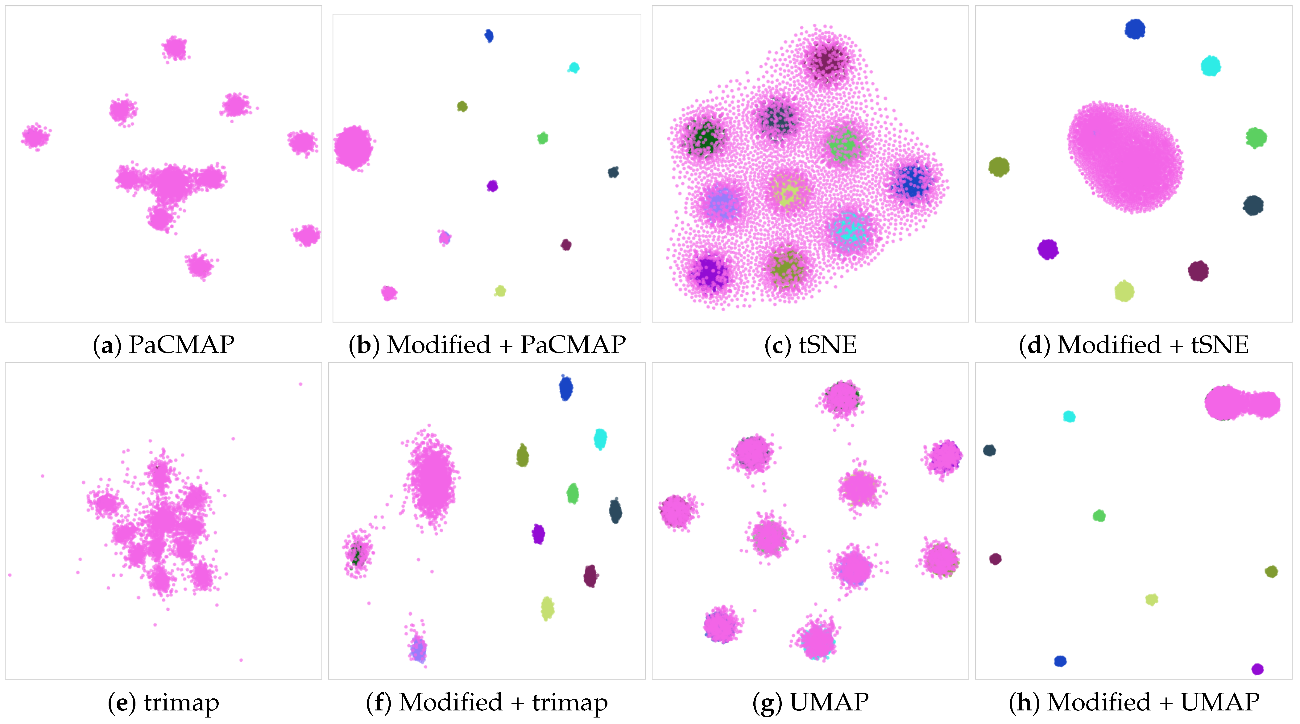
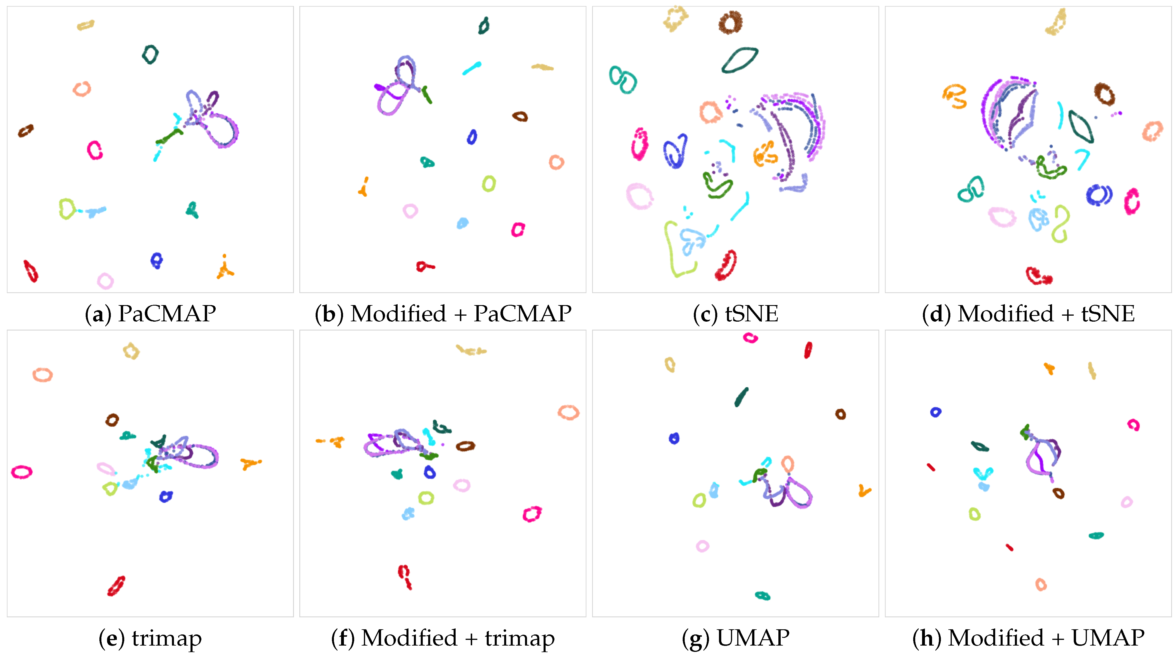
Figure 1 illustrates an example of the outcomes achievable with our method. The dataset consists of spheres belonging to eleven distinct classes, represented in a 101-dimensional space. When applying conventional dimensionality reduction (DR) algorithms, one of the classes invariably overlaps with the other clusters, as depicted in the first and third columns of the figure. However, by employing our manipulation scheme, we successfully separate a significant portion of these data points, leading to improved clustering outcomes, as evidenced in the second and fourth columns of the figure. By separating the data points more effectively, our method enhances the visualization and aids in better understanding the underlying patterns and relationships in the dataset. This demonstrates the effectiveness of our method in improving the results of DR algorithms for data clustering tasks.

Figure 1.
Dimensionality reduction of the spheres’ dataset using the different DR algorithms. Note that one of the classes, identified with the pink color, tends to overlap with the other clusters in the different cases. Our modifications effectively disentangle a substantial portion of the data points, resulting in a clearer and improved data visualization.
Our algorithm’s performance evaluation encompasses two distinct stages: the visualization of the dimensionality reduction (DR) datasets and the visualization of the document embeddings. In the first stage, we assess the accuracy metric of popular datasets commonly employed in articles on DR algorithms. In the second stage, we demonstrate the utility of our algorithm for projecting data, particularly document embeddings constructed using the doc2vec technique. We validate our algorithm’s capability to enhance the visualization of document embeddings, showcasing its efficacy in document data visualization.
3. Validation
Previous research has strongly suggested that the reduction in the dimensionality can significantly enhance the performance of clustering algorithms [29,30]. In our study, our primary objective is not to achieve the highest accuracy rate. Rather, we aim to evaluate the behavior of two different projections: one with the original data and another with the data modified by our algorithm. We want to ascertain the impact of our approach on the accuracy of the clustering algorithm after dimensionality reduction. To guarantee a thorough assessment, we plan to implement our methodology across multiple Dimensionality Reduction algorithms. While our preliminary evaluation entails comparing the accuracy of clustering using Support Vector Machines (SVM), we also broadened our analysis by incorporating several other clustering algorithms, including K-Nearest Neighbors (KNN) [34], Decision Trees (DT) [35], Extreme Gradient Boosting (XGBoost) [36], and Multilayer Perceptron (MLP) [37]. Among the most widely used nonlinear DR techniques in various applications are tSNE [13] and UMAP [16]. Additionally, emerging competitors have appeared recently, such as trimap [25] and PaCMAP [1]. We test those four algorithms.
3.1. Datasets
We selected a set of datasets commonly used in dimensionality reduction tests. Besides the widely known MNIST [38] and Fashion MNIST [39] models, we have also used other examples that combine both images and information from text: the tiny images dataset Cifar10 [40], Columbia images datasets (Coil20) [41], Human Activity Recognition using smartphones’ dataset (har) [42], Sentiment Labelled Sentences (sentiment) [43], Street Numbers (svhn) [44], USPS numbers dataset [45], FlickrMaterial10 [46], and the 20 Newsgroups dataset (20NG) [47]. All of them have multiple dimensions. We also included a specific dataset that is difficult to cluster using DR techniques, as demonstrated in Jeon et al. [26] and in Figure 1. This dataset, consisting of 10 K spheres in higher dimension, can be obtained from the code accompanying the paper [26]. The characteristics of the different datasets are shown in Table 1.

Table 1.
Features of the different datasets.
3.2. Experiment Setup
The majority of dimensionality reduction (DR) algorithms demonstrate a nondeterministic behavior, primarily due to certain steps, such as initialization, which may utilize random values to begin the selection of elements. Additionally, algorithms like tSNE and UMAP are highly reliant on their hyperparameters [48]. For this study, we intentionally refrained from hyperparameter tuning to maintain fairness and avoid bias in the results. Fine-tuning the hyperparameters separately for both the original and modified datasets could potentially skew the evaluation, and we wanted to ensure a fair comparison between the two. To address this challenge and guarantee the robustness of our approach, we executed each DR algorithm on a five-time basis independently. This allowed us to obtain multiple sets of projections for each dataset, thereby minimizing the impact of the nondeterministic behavior and the influence of the default hyperparameter values.
For the clustering task, we initially opted (later, we compared with other methods) for a linear Support Vector Machine (SVM) implementation by Boser et al. [49] with the ’multiclass’ parameter. The SVM algorithm was executed for 1000 iterations and evaluated using two themes: ’calibrated’ and ’not-calibrated,’ with a tenfold cross-validation approach. During each iteration, the SVM classifiers were trained on of the data, while the remaining constituted the testing data. To address the nondeterministic nature of the outcomes resulting from the inclusion of random variables in the execution of the SVM algorithm, we conducted five repetitions of each experiment for each data sample. The resulting accuracy values were then averaged to ensure the reliability and consistency of the clustering performance evaluation. By using multiple repetitions, we aim to obtain robust and stable performance metrics for the SVM-based clustering algorithm across different datasets and DR techniques.
To sum up, the process works as follows:
- For each dataset d, a transformation is applied using our algorithm, giving the transformed dataset .
- We project both d and using PaCMAP, tSNE, trimap, and UMAP.
- Each projected set is evaluated five times with the linear SVM method, and the results are averaged.
This procedure was repeated five times, and the results are the average of the five runs.
The obtained results for the PaCMAP algorithm are presented in Table 2. It is evident that in the majority of cases, the accuracy improves when our method is applied to the various models and the data is subsequently reduced to two dimensions using PaCMAP. Specifically, nine out of the eleven models exhibited an increase in their clustering accuracy.
Table 2.
Impact of the vector manipulation algorithm on the PaCMAP DR method for clustering using SVM. The center column displays the accuracy of the clustering algorithm when no vector manipulation is applied to the data, while the rightmost column shows the accuracy when our manipulation approach is applied. Notably, in the majority of the cases (9 out of 11), the accuracy improves.
The outcomes for the other dimensionality reduction (DR) algorithms exhibit similar trends. For the tSNE algorithm, we observe improvements in 7 out of the 11 models, as depicted in Table 3. The trimap algorithm does not work for the 20NG dataset (an error occurred that we did not further investigate ). Nonetheless, the majority of the models (8 out of 10) also improve, with a behavior similar to that of PaCMAP, as indicated in Table 4. Similarly, the UMAP yields comparable results, with 8 out of the 11 models experiencing improved clustering accuracy, as shown in Table 5.
Table 3.
tSNE accuracy without (center) and with (right) the algorithm. In this case, 7 out of the 11 models improve the result.
Table 4.
Accuracy obtained using trimap dimensionality reduction. The center column shows the results without our method, while the rightmost use our algorithm. trimap breaks for the 20NG model. In this case, we obtain an improvement in 8 out of the 10 models.
Table 5.
Accuracy obtained using UMAP. The center column shows the results without our method, while the rightmost use our algorithm. Here, we obtained an improvement in 8 out of the 11 models.
Notably, the PaCMAP algorithm, as demonstrated in [1], is less sensitive to hyperparameters. While we anticipate that better results might be obtained through proper hyperparameter fine-tuning for the other methods, we deliberately kept the experiments as neutral as possible to avoid unintended bias.
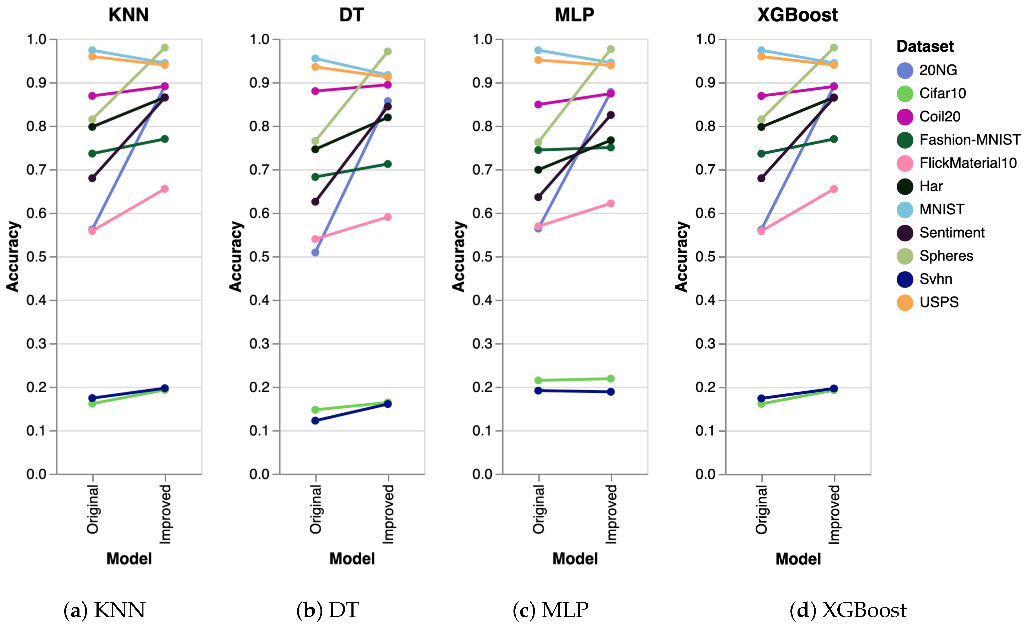
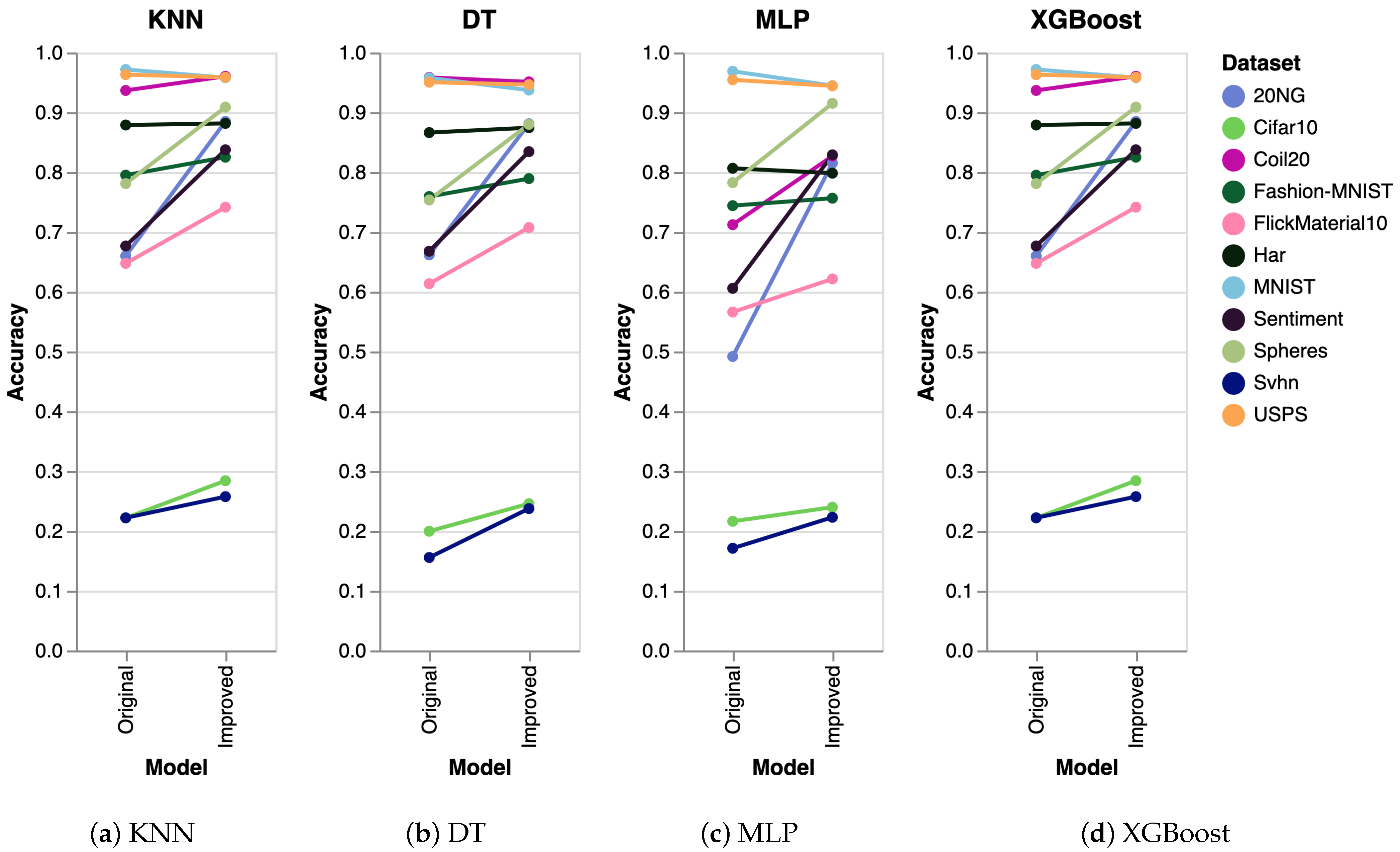
To further validate the performance of our algorithm, we conducted extra experiments using several other algorithms, including K-Nearest Neighbors (KNN), Decision Trees (DT), Multilayer Perceptron (MLP), and Extreme Gradient Boosting (XGBoost). The results obtained were consistent across all algorithms. The experimental setup was identical to that used for SVM, where we generated five datasets and executed the clustering algorithm five times on each dataset. The reported results represent the mean accuracy of these runs, visualized as slope charts in Figure 2 for PaCMAP. Analogously, we have also analyzed the accuracy for the other DR techniques, as shown in Figure 3 (trimap), Figure 4 (tSNE), and Figure 5 (UMAP).
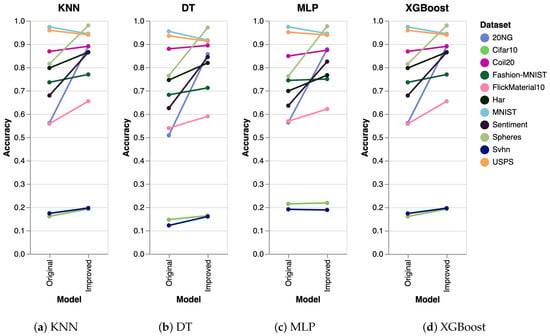
Figure 2.
Comparing other clustering algorithms for the PaCMAP DR algorithm. The results are equivalent to the ones obtained with SVM.
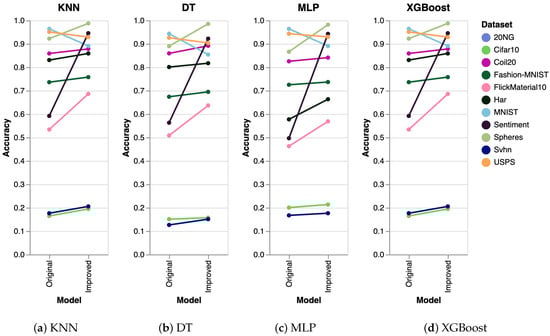
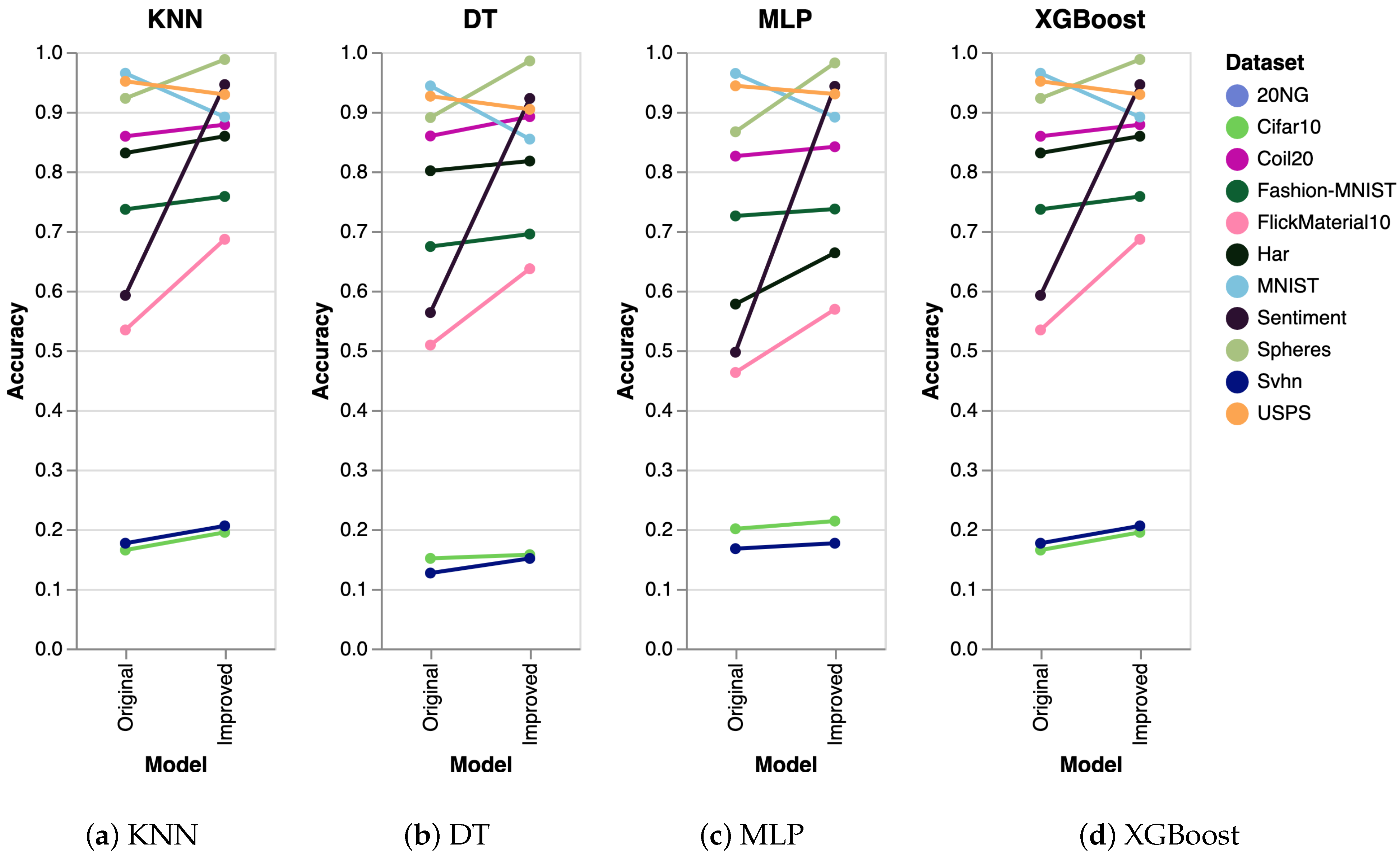
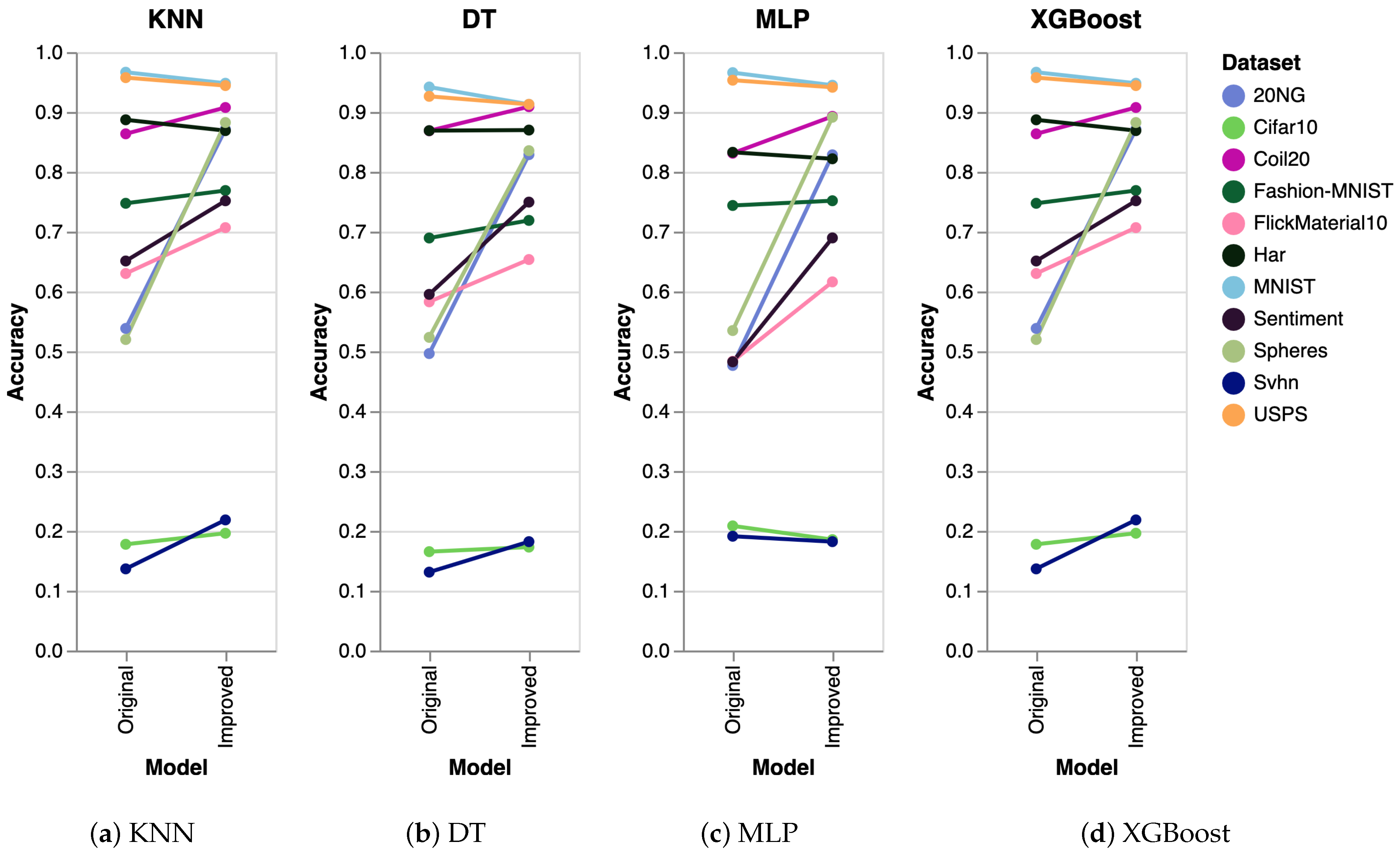
Figure 3.
Evaluation of trimap clustering using KNN, DT, MLP, and XGBoost. As in the previous case, the results are analogous to the ones obtained with SVM.
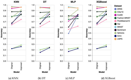
Figure 4.
Results obtained with the additional clustering algorithms for tSNE.
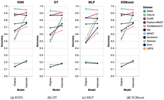
Figure 5.
Analysis of the UMAP DR data. The additional clustering algorithms also work similarly to the SVM.
To provide further insights into the performance of the algorithms, we compiled a summary of the percentages of the improvement in Table 6. The table reveals that our vector manipulation strategy improves the clustering accuracy for the majority of datasets. However, there are two datasets, namely MNIST and USPS, where our approach does not yield an improvement. In these cases, the accuracy decreases, albeit by a small amount for all DR algorithms. For the USPS model, the average accuracy reduction is consistently less than across all DR methods. Similarly, for the MNIST, the decrease is slightly larger but remains below . And the improvements can be considerable for some models, scaling up to more than for 20NG, the model that seems to benefit more from our approach.
Table 6.
The table presents a comparative analysis of the enhancements achieved through various Dimensionality Reduction (DR) techniques with our modification method. It displays the mean improvement obtained by employing five distinct clustering approaches. The models that demonstrate an improvement are highlighted in blue, while those that do not are highlighted in red. It is noteworthy that some models, which exhibit no improvement, are consistent across all DR techniques. Although these models exhibit a decline in accuracy, the magnitude of such reductions is negligible.
We can visually inspect the cases that exhibit no improvement. For instance, the USPS model does not enhance across any of the employed DR algorithms following our modification. Notwithstanding, the visualizations illustrate that the differences are not substantial, as shown in Figure 6.
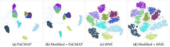
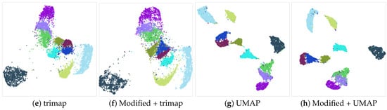
Figure 6.
Dimensionality reduction of the USPS dataset utilizing different DR algorithms. The PaCMAP (a) exhibits good results with the original data. Applying our vector modification (b), although numerically inferior to the original, the clusters are not substantially changed. For the tSNE (c), the modified version may give poorer results due to the fragmentation of some of the clusters that can be seen in (d). trimap DR (e) is less effective than PaCMAP or UMAP at cluster separation. Our algorithm output (f) appears visually akin to the original version (e). Finally, UMAP (g) yields results similar to PaCMAP, with well-concentrated clusters and only minor instances of collision or overlap. In this case, the data modification in (h) causes slight proximity changes in a couple of clusters.
Another model that exhibits a good behavior with our system is the Coil20 model. In this case, the enhancement is common to all DR algorithms but tSNE. This improvement is evident in the projections obtained, shown in Figure 7. While certain classes remain clustered even after the modifications, several clusters that were previously either split or overlapped with others now form distinct and well-defined clusters after the modification. The tSNE appears to be comparatively less performant than the other DR algorithms.
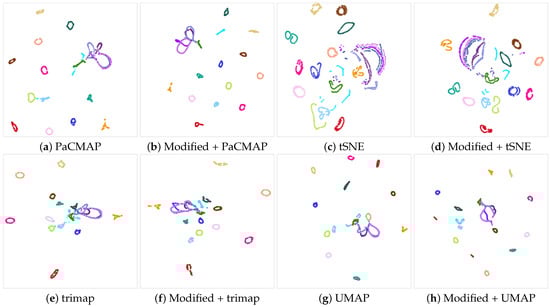
Figure 7.
The Coil20 dataset demonstrates enhanced clustering accuracy across all DR algorithms following our modification, except for the tSNE algorithm. This dataset contains 20 classes. Observe that the overall distribution of clusters improves after our modification (second and last column).
4. Document Visualization
In the previous section, we demonstrated that our method significantly improved the projections of several models commonly used in DR publications. In information visualization, DR algorithms are used in a wide range of scenarios to produce 2D layouts that enable further data exploration. We analyze one such case: document exploration.
Documents are complex data samples that are composed of words and can have a complex structure. We hereby use scientific articles as examples and have as a goal the creation of a 2D layout that shows the distribution of documents in a database.
To visualize documents, we need to transform those into simpler representations, such as vectors. There are many ways to make this transformation, one is to extract concepts from the text and represent those. Topic modeling has been previously used [50] to compare PhD theses, for example. Recent work has also used Latent Semantic Analysis-based representations followed by some DR algorithm [51,52] to obtain 2D representations of the documents.
Finally, Cartolabe is a tool for the exploration of massive document databases as point clouds with many interaction features. To achieve such layout, documents are transformed into vectors doc2vec [17] and projected using UMAP.
Following this idea, we build a dataset and explore how our vector transformation algorithm behaves when applied to doc2vec embeddings.
4.1. Document Embeddings
In numerous natural language tasks, a key component involves representing documents as fixed-size vectors. These representations capture the semantic essence of the texts in a way that can be processed by machines. Among the commonly employed representations, the bag-of-words [53] approach stands out. Another alternative is Latent Dirichlet Allocation (LDA) [54]. More advanced representations such as word2vec [55] and doc2vec [17] have been published recently. Unlike word2vec, which encodes individual words as floating-point vectors, doc2vec represents complete documents. The algorithm must first learn from a model containing textual data before it can create a doc2vec model. The models’ specificity greatly influences the quality of the representation. As there were no pre-existing models for representing scientific texts, our initial step involved the creation of such a model.
4.1.1. Doc2vec Model Training
We trained our doc2vec model on a massive dataset with 400 vector dimensions. The data used in the classification experiments is not included in our train set. Then, two different approaches were studied over the generated embeddings: (a) standard vectors with default values and (b) applying the L2 Norm on the previous item (a), as described previously.
Since doc2vec has the ability to be scaled with a large amount of data, we decided to explore the functionalities of this model by training it on large technical corpora. We decided to utilize S2ORC [56], which is a widespread corpus for natural language processing and text mining over scientific papers. That is, they have provided 136 M+ paper nodes with 12.7 M+ full-text papers and connected by 467 M+ citation edges by combining data from various sources with academic disciplines and identifying open-access papers. The minimum and the maximum number of tokens in our selected dataset varies from 1 to 287,400. We decided to select documents with at least 200 tokens to not be less than the smallest document in our test set.
For training purposes, since we focused on technical documents, we collected 341,891 documents with the size of ∼10 G in the fields of Engineering, Computer Science, Physics, and Math, among the provided data sources.
4.1.2. Synthetic Dataset Creation
Since there is no standard baseline to evaluate the similarity between lengthy scientific documents, exceeding 4000 tokens, as highlighted in [57], we created a synthetic dataset for this purpose. The dataset was curated by hand-picking articles from diverse disciplines and complementing them with a systematic selection of additional files from arxiv.org.
The construction of the synthetic dataset aimed to incorporate clearly differentiated clusters, exemplified by distinct fields such as Electrical Engineering and Molecular Visualization. Additionally, we sought to include similar fields, like Ambient Occlusion and Global Illumination, both of which are different techniques aiming to achieve similar goals in the domain of Computer Graphics.
Another key objective was to ensure a relatively large number of classes, as most existing baselines in the literature often involve only a few classes. During the collection of data from arxiv.org, we have observed a prevalent trend of recent papers in the field of Electrical Engineering employing deep learning techniques (EE22). Consequently, we purposefully selected an additional cluster of articles in the same field, albeit from a previous period (2015), referred to as EE15. This decision allowed further analysis to determine whether older articles formed a distinct cluster and whether newer papers demonstrated increased similarity to the Artificial Intelligence (AI) cluster.
After the selection process, the final synthetic dataset consisted of 278 documents distributed across 13 classes. Each class comprised approximately 20 papers. The categories and the number of papers in each class are outlined in Table 7.
Table 7.
Contents of the different clusters.
4.1.3. Data Preprocessing
To create the document embeddings, we followed this process: We first converted the PDF documents into text format, and then we removed the author, image, table, and caption information, along with the references, acknowledgements, and formulas. In addition, we eliminated the sentences with less than three tokens. We then followed the preprocessing pipelines on the raw data from [58] that lowercases, tokenizes, and de-accents the sentences. Finally, stop words were removed using [59]. An additional task was performed on the test sets. All these steps, as well as the posterior executions, used Python3.
This is the input that was given to the doc2vec algorithm. doc2vec, introduced by [17] and inspired by word2vec [55] is considered as one of the NLP approaches to representing documents as vectors. Recent experiments have showcased its applicability in scientific document comparison, when combined with cosine similarity [60]. Furthermore, doc2vec has proven effective for visually exploring corpora of scientific documents through dimensionality reduction techniques [15]. In the doc2vec technique, two matrices, namely D and W, were built. Each column in D corresponded to the mapping of a paragraph to a unique vector. In W, each column represented a mapping of every word to a unique vector. To predict the next word in a given context, both the paragraph vector and word vectors were concatenated. As usual, we treated each document as a paragraph when employing the doc2vec algorithm.
4.1.4. Clusters’ Quality Analysis
To assess the quality of the hand-picked clusters, we conducted an experiment using cosine similarity. We utilized the preprocessing pipeline outlined above, and then, we compared the cosine similarity of each document to any other in the data set, excluding self-comparisons to maintain fairness in the evaluation. The obtained results are presented in Table 8.
Table 8.
The average similarity scores for the different clusters in the technical documents’ dataset. Notice how the inner average similarity of each class is consistently lower than the average similarities against other classes, except for the HEAP (High-Energy Astrophysical Phenomena) and APG (Astrophysics of Galaxies) classes. This aligns with the fact that both classes are closely related and belong to the same arXiv superclass. Additionally, as anticipated, the Volume Rendering and Ambient Occlusion classes exhibit a high degree of similarity. In addition, we can also see that the Volume Rendering and Ambient Occlusion are very similar, as expected.
Considering the documents of each class as a cluster, we observed that we achieved higher average cosine similarity (coherency) within documents of the same cluster compared to the other clusters. Additionally, we observed that some clusters were more coherent than others. For instance, the Electrical Engineering 2022 cluster was more similar to the Artificial Intelligence (0.104) than the Electrical Engineering 2015 one (0.091). This aligned with our earlier observation that many recent Electrical Engineering articles often incorporate deep learning techniques. Furthermore, there was a notable cosine similarity between some clusters such as Higher Energy Astrophysics and Astrophysics Galaxies (0.248 self and 0.249 for AG) as well as dissimilarity in some others, namely Ambient Occlusion (0.39 for self) and Electrical Engineering (0.095, 0.011 in 2015 and 2022 respectively). These findings were consistent with our expectations. Another result that confirmed the expected behavior of our approach was the similarity between related areas, such as Global Illumination and Ambient Occlusion, both of which addressed a similar goal (realistic image synthesis), through different techniques. Molecular Visualization in Virtual Reality, which extensively employed Computer Graphics techniques, exhibited a higher similarity to the Computer Graphics—Ambient Occlusion cluster. Similarly, the Volume Rendering had the Virtual Reality cluster as a closer one.
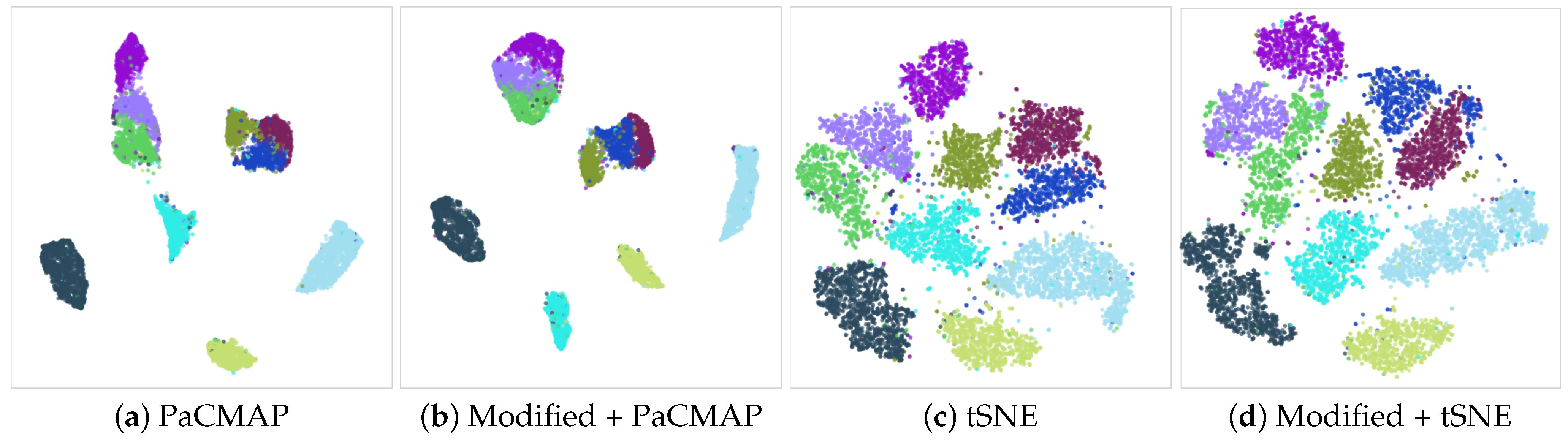
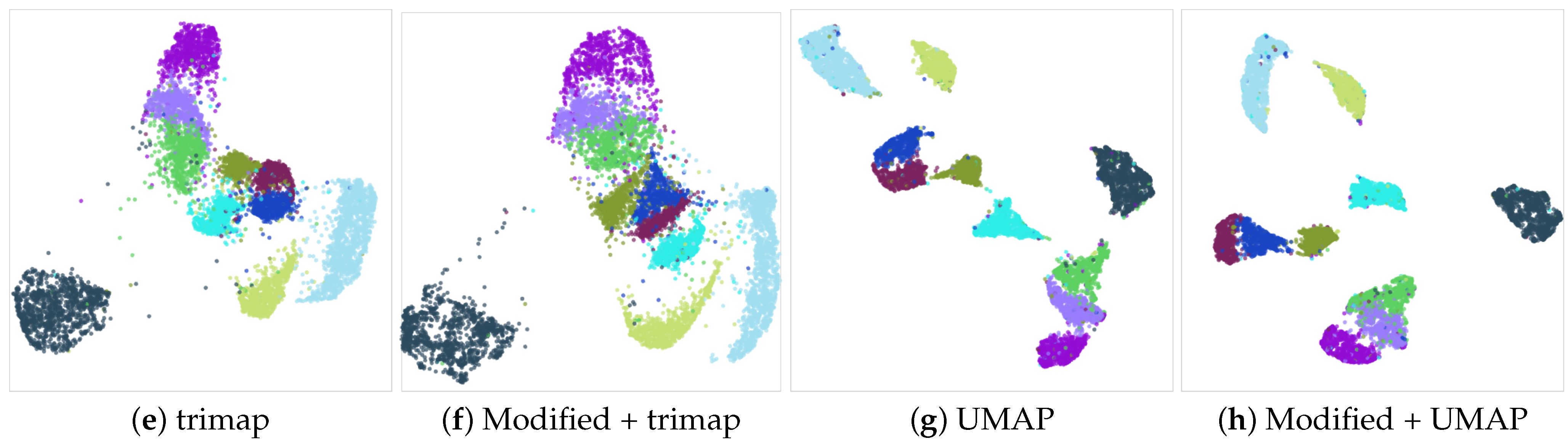
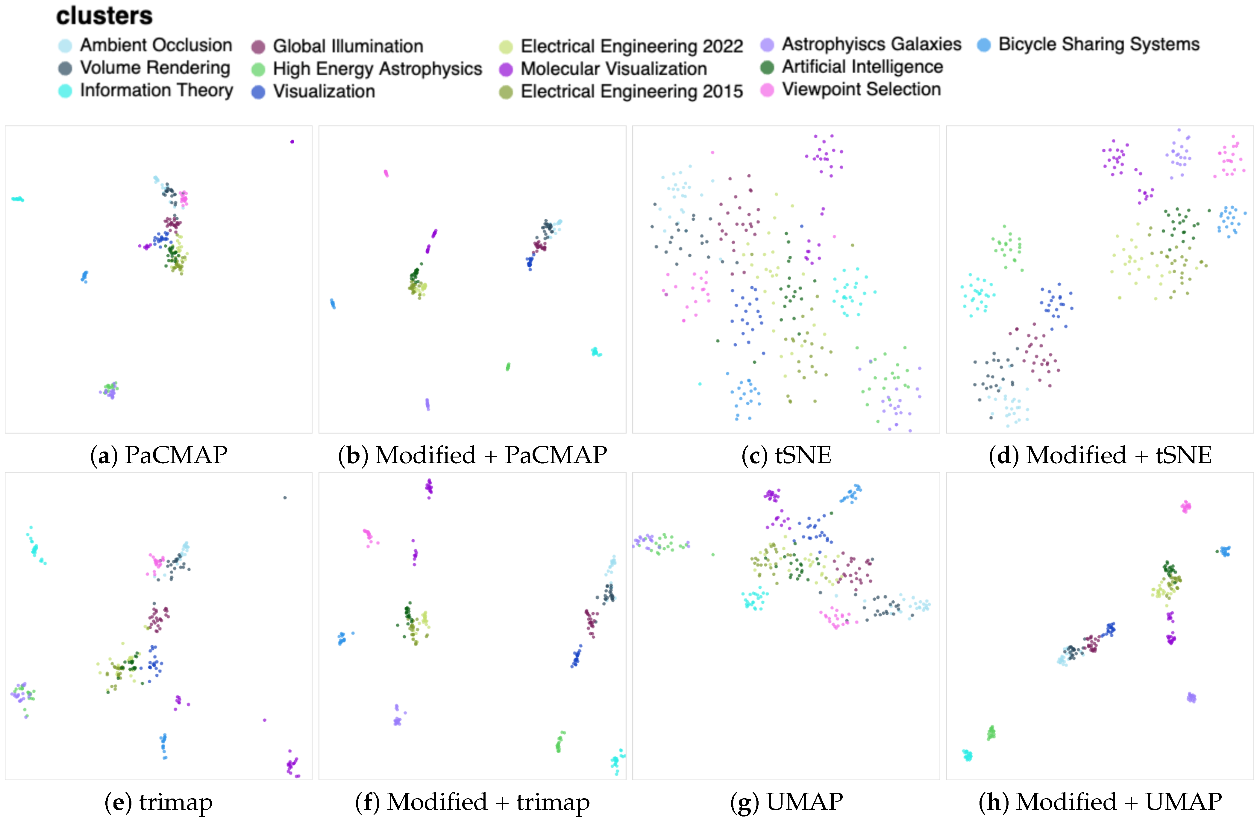
When applying the PaCMAP for dimensionality reduction on the mentioned data, it was evident from Figure 8a that not all areas were adequately clustered into distinct and visible groups. Certain clusters appeared to be tightly packed together, and the algorithm encountered difficulties in effectively segregating them. Nonetheless, it is noteworthy that the clustering pattern was in accordance with our previous observations. Astrophysics clusters were mixed at the bottom, while certain groups, like Information Theory and Bicycle Sharing Systems, were distinctly positioned away from the central group of Computer Graphics-related clusters. Despite these similarities, the algorithm still failed to create more well-defined clusters.
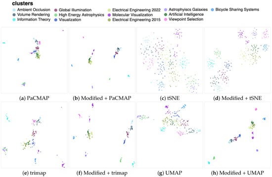
Figure 8.
The documents dataset indicated clear improvements in all the DR algorithms. Please note that the modified versions generated projections with a better separation between clusters.
However, with the application of the improved version of the algorithm, shown in Figure 8b, significant improvements were evident. The enhanced version effectively divided the clusters, such as the two Astrophysics groups. Furthermore, the Electrical Engineering groups were now distinct from the others. A clear cluster for Viewpoint Selection was also observable. This demonstrates the positive impact of our modifications on the algorithm’s performance, particularly when dealing with a challenging dataset that includes papers from the Computer Graphics field and closely related areas.
In addition, the improved results are also observed in the case of other DR algorithms, as depicted in Figure 8d,f,h. For instance, the tSNE algorithm exhibited more sparse clusters, which could potentially be further optimized with different numbers of neighbors. Nonetheless, as previously mentioned, we retained the default parameters of the DR algorithms to prevent any unfair fine-tuning.
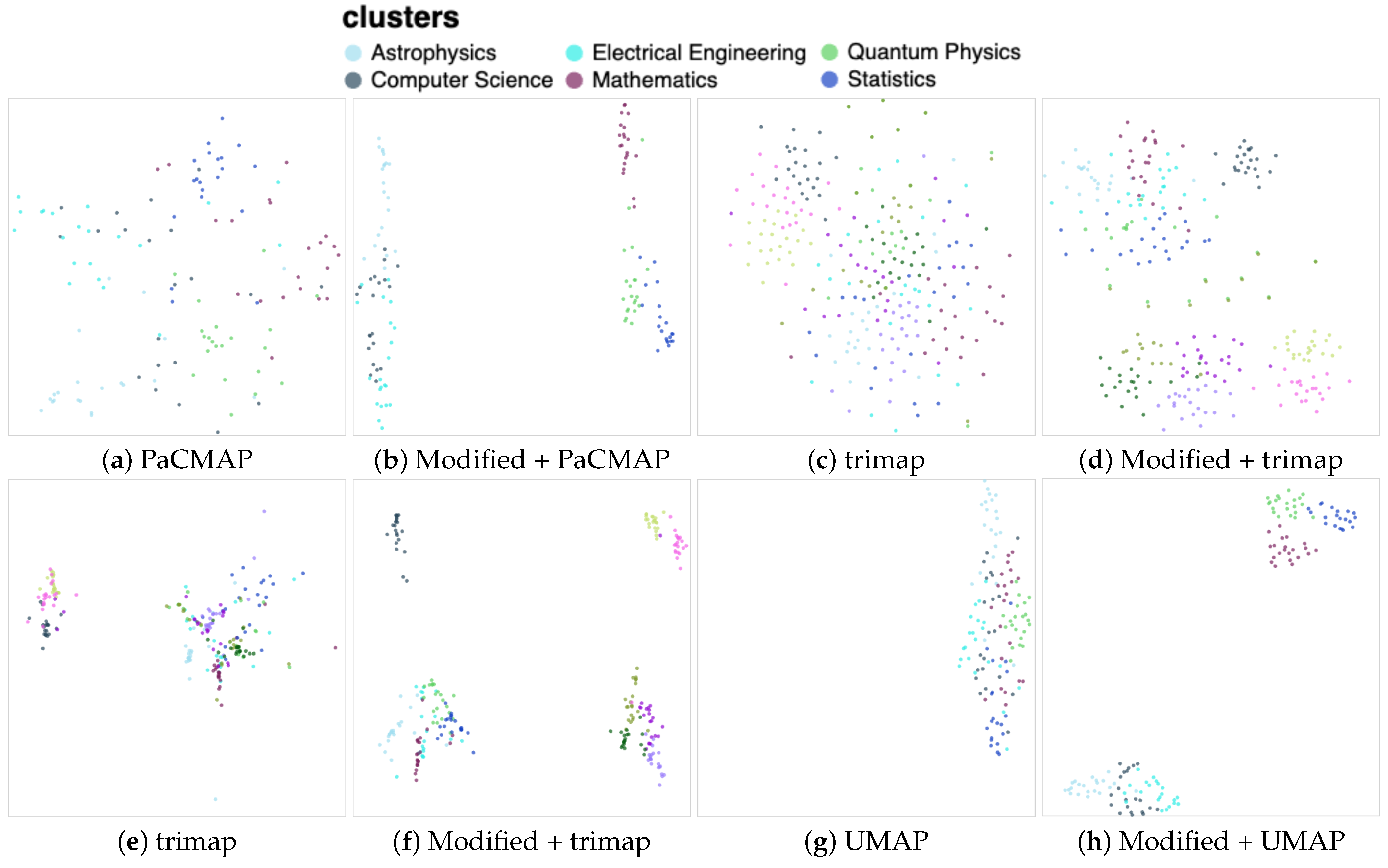
In the second experiment, we present the results from a new dataset that differed from the carefully curated one used previously. Instead of a deliberately designed dataset, this collection was constructed by selecting the last 21 articles available arXiv database on different areas. The dataset comprised six categories: Astrophysics, Computer Science, Electrical Engineering, Mathematics, Quantum Physics, and Statistics. For each category, the last 21 available articles were downloaded.
The documents from this dataset underwent the same preprocessing pipeline as described earlier. Subsequently, we conducted similar experiments to evaluate clustering performance. The results obtained from these experiments are illustrated in Figure 9. In contrast to the previous dataset, here, the DR algorithms demonstrated less success in identifying clusters. These results were enhanced through our data manipulation, leading to the increased visibility of certain clusters, for example with PaCMAP (b). The modified vectors exhibited improved performance with other DR algorithms as well. This observation was evident from Figure 9d,f,h, where the distinct clusters were more distinctly isolated following the modification of the input data. However, they did not exhibit the same level of clarity as observed in the previous dataset.
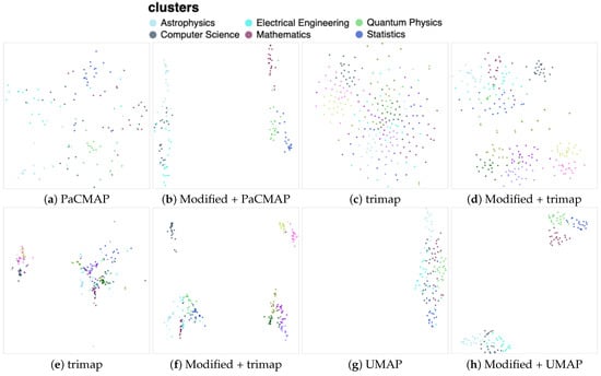
Figure 9.
This document set was not as clearly separated by any of the DR techniques. With our modification, the trimap demonstrated superior performance in achieving cluster separation. The other techniques also improved, but the clustering separations were not obvious.
5. Conclusions and Future Work
5.1. Conclusions
We introduced a novel method designed to enhance the outcomes of DR algorithms when dealing with high-dimensional datasets. The proposed technique is centered around facilitating visual exploration and has been validated through the utilization of clustering algorithms on the resultant data. The key advantage of our approach lies in its complete automation, without requiring fine-tuning, and its compatibility with various DR algorithms. Furthermore, the process requires only a global data analysis, incurring linear computational costs, thereby making it well-suited for standard computers. The data processing, implemented in C++, takes mere milliseconds to execute on a laptop. Another advantage of our technique is that it achieves positive results for a variety of DR methods. These results were obtained without any hyperparameter tweaking of the DR algorithms. We analyzed the efficacy of our method through the use of conventional models featured in articles that analyze DR algorithms. Our system showed favorable outcomes for the majority of such models. Furthermore, we successfully employed the same approach for visualizing documents using document embeddings.
5.2. Discussion
The presented algorithm holds the potential for application in any visualization system that employs DR to create 2D layouts, such as [2,12,15,23]. Notably, we refrained from investigating 3D layouts due to their less common usage and known disadvantages for users [27].
One limitation to acknowledge is that the algorithm did not uniformly improve the clustering for all models. Nevertheless, we intend to conduct further investigations into these results, particularly since two models that did not demonstrate improved clustering were consistent across all DR algorithms. It is a well-established fact that the IDF may produce significantly large values for infrequent terms. However, upon analyzing the IDF values generated for all models in our experiments, we did not encounter any issues. We postulate that this could be attributed to our use of weights instead of terms. Specifically, for document sets, we employed 400-dimensional embeddings. While this may pose a challenge for significantly larger dimensions, 400 dimensions are adequate for accurately representing extensive documents, such as scholarly articles.
5.3. Future Work
In the future, we aim to investigate various extensions. Primarily, we intend to evaluate the performance of our methodology using embeddings besides doc2vec. While we anticipate that the algorithm will function effectively with BERT [18] or Longformer [61] embeddings, a comprehensive analysis is warranted. Additionally, we plan to delve deeper into the reasons for the lack of improvement in certain models. Our conjecture is that models with distinctly separated data in high-dimensional space may not necessitate this enhancement. However, this can only be confirmed using labeled data, making the analysis of non-labeled data challenging.
Author Contributions
Conceptualization, B.R., P.H. and P.-P.V.; methodology, B.R., P.H. and P.-P.V.; software, B.R. and P.-P.V.; validation, B.R.; formal analysis, B.R. and P.-P.V.; investigation, B.R., P.H. and P.H.; resources, B.R. and P.-P.V.; data curation, B.R. and P.-P.V.; writing—original draft preparation, B.R. and P.-P.V.; writing—review and editing, B.R., P.H. and P.-P.V.; visualization, P.-P.V.; supervision, P.H. and P.-P.V.; project administration, P.-P.V.; funding acquisition, P.-P.V. All authors have read and agreed to the published version of the manuscript.
Funding
This research was funded by PID2021-122136OB-C21 from the Ministerio de Ciencia e Innovación, Spain, by 839 FEDER (EU) funds.
Data Availability Statement
The data used in our validation experiments are public, and we provided the references where they can be obtained.
Conflicts of Interest
The authors declare no conflict of interest. The funders had no role in the design of the study; in the collection, analyses, or interpretation of data; in the writing of the manuscript; or in the decision to publish the results.
Abbreviations
The following abbreviations are used in this manuscript:
| DR | Dimensionality Reduction |
| DT | Decision Trees |
| KNN | K-Nearest Neighbors |
| MLP | Multilayer Perceptron |
| PaCMAP | Pairwise Controlled Manifold Approximation Projection |
| SVM | Support Vector Machines |
| trimap | Large-scale Dimensionality Reduction Using Triplets |
| t-SNE | t-Distributed Stochastic Neighbor Embedding |
| UMAP | Uniform Manifold Approximation and Projection |
| XGBoost | Extreme Gradient Boosting |
References
- Wang, Y.; Huang, H.; Rudin, C.; Shaposhnik, Y. Understanding how dimension reduction tools work: An empirical approach to deciphering t-SNE, UMAP, TriMAP, and PaCMAP for data visualization. J. Mach. Learn. Res. 2021, 22, 9129–9201. [Google Scholar]
- Hinterreiter, A.; Steinparz, C.; Schöfl, M.; Stitz, H.; Streit, M. Projection path explorer: Exploring visual patterns in projected decision-making paths. ACM Trans. Interact. Intell. Syst. 2021, 11, 22. [Google Scholar] [CrossRef]
- Becht, E.; McInnes, L.; Healy, J.; Dutertre, C.A.; Kwok, I.W.; Ng, L.G.; Ginhoux, F.; Newell, E.W. Dimensionality reduction for visualizing single-cell data using UMAP. Nat. Biotechnol. 2019, 37, 38–44. [Google Scholar] [CrossRef] [PubMed]
- Vlachos, M.; Domeniconi, C.; Gunopulos, D.; Kollios, G.; Koudas, N. Non-linear dimensionality reduction techniques for classification and visualization. In Proceedings of the Eighth ACM SIGKDD International Conference on Knowledge Discovery and Data Mining, Edmonton, AB, Canada, 23–26 July 2002; pp. 645–651. [Google Scholar]
- Cunningham, J.P.; Ghahramani, Z. Linear dimensionality reduction: Survey, insights, and generalizations. J. Mach. Learn. Res. 2015, 16, 2859–2900. [Google Scholar]
- Lee, J.A.; Verleysen, M. Nonlinear Dimensionality Reduction; Springer: Berlin/Heidelberg, Germany, 2007; Volume 1. [Google Scholar]
- Ayesha, S.; Hanif, M.K.; Talib, R. Overview and comparative study of dimensionality reduction techniques for high dimensional data. Inf. Fusion 2020, 59, 44–58. [Google Scholar] [CrossRef]
- Sorzano, C.O.S.; Vargas, J.; Montano, A.P. A survey of dimensionality reduction techniques. arXiv 2014, arXiv:1403.2877. [Google Scholar]
- Engel, D.; Hüttenberger, L.; Hamann, B. A survey of dimension reduction methods for high-dimensional data analysis and visualization. In Proceedings of the Visualization of Large and Unstructured Data Sets: Applications in Geospatial Planning, Modeling and Engineering-Proceedings of IRTG 1131 Workshop, Kaiserslautern, Germany, 10–11 June 2011; Schloss Dagstuhl-Leibniz-Zentrum fuer Informatik: Wadern, Germany, 2012. [Google Scholar]
- Van Der Maaten, L.; Postma, E.; Van den Herik, J. Dimensionality reduction: A comparative. J. Mach. Learn Res. 2009, 10, 66–71. [Google Scholar]
- Sedlmair, M.; Brehmer, M.; Ingram, S.; Munzner, T. Dimensionality Reduction in the Wild: Gaps and Guidance; Tech. Rep. TR-2012-03; Department of Computer Science, University of British Columbia: Vancouver, BC, Canada, 2012. [Google Scholar]
- Huang, H.; Wang, Y.; Rudin, C.; Browne, E.P. Towards a comprehensive evaluation of dimension reduction methods for transcriptomic data visualization. Commun. Biol. 2022, 5, 719. [Google Scholar] [CrossRef]
- Van der Maaten, L.; Hinton, G. Visualizing data using t-SNE. J. Mach. Learn. Res. 2008, 9, 2579–2605. [Google Scholar]
- Wattenberg, M.; Viégas, F.; Johnson, I. How to use t-SNE effectively. Distill 2016, 1, e2. [Google Scholar] [CrossRef]
- Caillou, P.; Renault, J.; Fekete, J.D.; Letournel, A.C.; Sebag, M. Cartolabe: A web-based scalable visualization of large document collections. IEEE Comput. Graph. Appl. 2020, 41, 76–88. [Google Scholar] [CrossRef] [PubMed]
- McInnes, L.; Healy, J.; Melville, J. UMAP: Uniform Manifold Approximation and Projection for Dimension Reduction. arXiv 2020, arXiv:stat.ML/1802.03426. [Google Scholar]
- Le, Q.; Mikolov, T. Distributed representations of sentences and documents. In Proceedings of the International Conference on Machine Learning, Reykjavik, Iceland, 22–25 April 2014; pp. 1188–1196. [Google Scholar]
- Kenton, J.D.M.W.C.; Toutanova, L.K. BERT: Pre-training of Deep Bidirectional Transformers for Language Understanding. In Proceedings of the NAACL-HLT, Minneapolis, MN, USA, 2–7 June 2019; pp. 4171–4186. [Google Scholar]
- Silva, D.; Bacao, F. MapIntel: Enhancing Competitive Intelligence Acquisition through Embeddings and Visual Analytics. In Proceedings of the EPIA Conference on Artificial Intelligence, Lisbon, Portugal, 31 August–2 September 2022; Springer: Berlin/Heidelberg, Germany, 2022; pp. 599–610. [Google Scholar]
- Abdullah, S.S.; Rostamzadeh, N.; Sedig, K.; Garg, A.X.; McArthur, E. Visual analytics for dimension reduction and cluster analysis of high dimensional electronic health records. Informatics 2020, 7, 17. [Google Scholar] [CrossRef]
- Humer, C.; Heberle, H.; Montanari, F.; Wolf, T.; Huber, F.; Henderson, R.; Heinrich, J.; Streit, M. ChemInformatics Model Explorer (CIME): Exploratory analysis of chemical model explanations. J. Cheminform. 2022, 14, 21. [Google Scholar] [CrossRef] [PubMed]
- Burch, M.; Kuipers, T.; Qian, C.; Zhou, F. Comparing dimensionality reductions for eye movement data. In Proceedings of the 13th International Symposium on Visual Information Communication and Interaction, Eindhoven, The Netherlands, 8–10 December 2020; pp. 1–5. [Google Scholar]
- Dorrity, M.W.; Saunders, L.M.; Queitsch, C.; Fields, S.; Trapnell, C. Dimensionality reduction by UMAP to visualize physical and genetic interactions. Nat. Commun. 2020, 11, 1537. [Google Scholar] [CrossRef] [PubMed]
- Tang, J.; Liu, J.; Zhang, M.; Mei, Q. Visualizing large-scale and high-dimensional data. In Proceedings of the 25th International Conference on World Wide Web, Montreal, QC, Canada, 11–15 April 2016; pp. 287–297. [Google Scholar]
- Amid, E.; Warmuth, M.K. TriMap: Large-scale dimensionality reduction using triplets. arXiv 2019, arXiv:1910.00204. [Google Scholar]
- Jeon, H.; Ko, H.K.; Lee, S.; Jo, J.; Seo, J. Uniform Manifold Approximation with Two-phase Optimization. In Proceedings of the 2022 IEEE Visualization and Visual Analytics (VIS), Oklahoma City, OK, USA, 16–21 October 2022; pp. 80–84. [Google Scholar]
- Sedlmair, M.; Munzner, T.; Tory, M. Empirical guidance on scatterplot and dimension reduction technique choices. IEEE Trans. Vis. Comput. Graph. 2013, 19, 2634–2643. [Google Scholar] [CrossRef]
- Espadoto, M.; Martins, R.M.; Kerren, A.; Hirata, N.S.; Telea, A.C. Toward a quantitative survey of dimension reduction techniques. IEEE Trans. Vis. Comput. Graph. 2019, 27, 2153–2173. [Google Scholar] [CrossRef]
- Olobatuyi, K.; Parker, M.R.; Ariyo, O. Cluster weighted model based on TSNE algorithm for high-dimensional data. Int. J. Data Sci. Anal. 2023. [Google Scholar] [CrossRef]
- Allaoui, M.; Kherfi, M.L.; Cheriet, A. Considerably improving clustering algorithms using UMAP dimensionality reduction technique: A comparative study. In Proceedings of the International Conference on Image and Signal Processing, Marrakesh, Morocco, 4–6 June 2020; Springer: Berlin/Heidelberg, Germany, 2020; pp. 317–325. [Google Scholar]
- Church, K.; Gale, W. Inverse document frequency (idf): A measure of deviations from poisson. In Natural Language Processing Using Very Large Corpora; Springer: Berlin/Heidelberg, Germany, 1999; pp. 283–295. [Google Scholar]
- Sparck Jones, K. A statistical interpretation of term specificity and its application in retrieval. J. Doc. 1972, 28, 11–21. [Google Scholar] [CrossRef]
- Robertson, S. Understanding inverse document frequency: On theoretical arguments for IDF. J. Doc. 2004, 60, 503–520. [Google Scholar] [CrossRef]
- Cover, T.; Hart, P. Nearest neighbor pattern classification. IEEE Trans. Inf. Theory 1967, 13, 21–27. [Google Scholar] [CrossRef]
- Quinlan, J.R. Induction of Decision Trees. Mach. Learn. 1986, 1, 81–106. [Google Scholar] [CrossRef]
- Chen, T.; Guestrin, C. XGBoost: A Scalable Tree Boosting System. In Proceedings of the 22nd ACM SIGKDD International Conference on Knowledge Discovery and Data Mining, San Francisco, CA, USA, 13–17 August 2016; KDD’16. ACM: New York, NY, USA, 2016; pp. 785–794. [Google Scholar] [CrossRef]
- Haykin, S. Neural Networks: A Comprehensive Foundation; Prentice Hall PTR: London, UK, 1994. [Google Scholar]
- LeCun, Y.; Cortes, C. The MNIST Database of Handwritten Digits. 1998. Available online: http://yann.lecun.com/exdb/mnist/ (accessed on 15 May 2023).
- Xiao, H.; Rasul, K.; Vollgraf, R. Fashion-mnist: A novel image dataset for benchmarking machine learning algorithms. arXiv 2017, arXiv:1708.07747. [Google Scholar]
- Krizhevsky, A.; Hinton, G. Learning Multiple Layers of Features from Tiny Images. 2009. Available online: https://www.cs.toronto.edu/~kriz/ (accessed on 27 July 2023).
- Nene, S.A.; Nayar, S.K.; Murase, H. Columbia Object Image Library (Coil-20); Technical Report; Columbia University: New York, NY, USA, 1996. [Google Scholar]
- Reyes-Ortiz, J.; Anguita, D.; Ghio, A.; Oneto, L.; Parra, X. Human Activity Recognition Using Smartphones. UCI Mach. Learn. Repos. 2012. [Google Scholar] [CrossRef]
- Kotzias, D. Sentiment Labelled Sentences. UCI Mach. Learn. Repos. 2015. [Google Scholar] [CrossRef]
- Yuval, N. Reading digits in natural images with unsupervised feature learning. In Proceedings of the NIPS Workshop on Deep Learning and Unsupervised Feature Learning, Granada, Spain, 12–17 December 2011. [Google Scholar]
- Hull, J.J. A database for handwritten text recognition research. IEEE Trans. Pattern Anal. Mach. Intell. 1994, 16, 550–554. [Google Scholar] [CrossRef]
- Sharan, L.; Rosenholtz, R.; Adelson, E. Material perception: What can you see in a brief glance? J. Vis. 2009, 9, 784. [Google Scholar] [CrossRef]
- Lang, K. 20 Newsgroups Dataset. Available online: https://www.cs.cmu.edu/afs/cs/project/theo-20/www/data/news20.html (accessed on 15 May 2023).
- Cutura, R.; Holzer, S.; Aupetit, M.; Sedlmair, M. VisCoDeR: A tool for visually comparing dimensionality reduction algorithms. In Proceedings of the Esann, Bruges, Belgium, 25–27 April 2018. [Google Scholar]
- Boser, B.E.; Guyon, I.M.; Vapnik, V.N. A Training Algorithm for Optimal Margin Classifiers. In Proceedings of the Fifth Annual Workshop on Computational Learning Theory, Pittsburgh, PA, USA, 27–29 July 1992; COLT’92. Association for Computing Machinery: New York, NY, USA, 1992; pp. 144–152. [Google Scholar] [CrossRef]
- Chuang, J.; Ramage, D.; Manning, C.; Heer, J. Interpretation and trust: Designing model-driven visualizations for text analysis. In Proceedings of the SIGCHI Conference on Human Factors in Computing Systems, Austin, TX, USA, 5–10 May 2012; pp. 443–452. [Google Scholar]
- Landauer, T.K.; Laham, D.; Derr, M. From paragraph to graph: Latent semantic analysis for information visualization. Proc. Natl. Acad. Sci. USA 2004, 101, 5214–5219. [Google Scholar] [CrossRef]
- Kim, K.; Lee, J. Sentiment visualization and classification via semi-supervised nonlinear dimensionality reduction. Pattern Recognit. 2014, 47, 758–768. [Google Scholar] [CrossRef]
- Harris, Z.S. Distributional structure. Word 1954, 10, 146–162. [Google Scholar] [CrossRef]
- Blei, D.M.; Ng, A.Y.; Jordan, M.I. Latent dirichlet allocation. J. Mach. Learn. Res. 2003, 3, 993–1022. [Google Scholar]
- Mikolov, T.; Chen, K.; Corrado, G.; Dean, J. Efficient Estimation of Word Representations in Vector Space. arXiv 2013, arXiv:1301.3781. [Google Scholar]
- Lo, K.; Wang, L.L.; Neumann, M.; Kinney, R.; Weld, D. S2ORC: The Semantic Scholar Open Research Corpus. In Proceedings of the 58th Annual Meeting of the Association for Computational Linguistics, Online, 5–10 July 2020; Association for Computational Linguistics: Toronto, ON Canada, 2020; pp. 4969–4983. [Google Scholar] [CrossRef]
- Alvarez, J.E.; Bast, H. A Review of Word Embedding and Document Similarity Algorithms Applied to Academic Text. Bachelor Thesis, University of Freiburg, Freiburg im Breisgau, Germany, 2017. [Google Scholar]
- Rehurek, R.; Sojka, P. Gensim–Python Framework for Vector Space Modelling; NLP Centre, Faculty of Informatics, Masaryk University: Brno, Czech Republic, 2011; Volume 3. [Google Scholar]
- Bird, S.; Klein, E.; Loper, E. Natural Language Processing with Python: Analyzing Text with the Natural Language Toolkit; O’Reilly Media, Inc.: Sebastopol, CA, USA, 2009. [Google Scholar]
- Gómez, J.; Vázquez, P.P. An Empirical Evaluation of Document Embeddings and Similarity Metrics for Scientific Articles. Appl. Sci. 2022, 12, 5664. [Google Scholar] [CrossRef]
- Beltagy, I.; Peters, M.E.; Cohan, A. Longformer: The long-document transformer. arXiv 2020, arXiv:2004.05150. [Google Scholar]
Disclaimer/Publisher’s Note: The statements, opinions and data contained in all publications are solely those of the individual author(s) and contributor(s) and not of MDPI and/or the editor(s). MDPI and/or the editor(s) disclaim responsibility for any injury to people or property resulting from any ideas, methods, instructions or products referred to in the content. |
© 2023 by the authors. Licensee MDPI, Basel, Switzerland. This article is an open access article distributed under the terms and conditions of the Creative Commons Attribution (CC BY) license (https://creativecommons.org/licenses/by/4.0/).