Abstract
Extracting effective features from high-dimensional datasets is crucial for determining the accuracy of regression and classification models. Model predictions based on causality are known for their robustness. Thus, this paper introduces causality into feature selection and utilizes Feature Selection based on NOTEARS causal discovery (FSNT) for effective feature extraction. This method transforms the structural learning algorithm into a numerical optimization problem, enabling the rapid identification of the globally optimal causality diagram between features and the target variable. To assess the effectiveness of the FSNT algorithm, this paper evaluates its performance by employing 10 regression algorithms and 8 classification algorithms for regression and classification predictions on six real datasets from diverse fields. These results are then compared with three mainstream feature selection algorithms. The results indicate a significant average decline of 54.02% in regression prediction achieved by the FSNT algorithm. Furthermore, the algorithm exhibits exceptional performance in classification prediction, leading to an enhancement in the precision value. These findings highlight the effectiveness of FSNT in eliminating redundant features and significantly improving the accuracy of model predictions.
1. Introduction
In order to reduce the computational cost of model classification or regression, it is desirable to select as few features as possible while ensuring estimation quality. Furthermore, utilizing all available features not only invalidates the model’s calculation [1] but also increases the likelihood of overfitting [2], consequently reducing the predictive accuracy. Feature selection is a fundamental and relatively straightforward strategy in data mining [3]. It should be noted that we focus solely on the correlation between variables, not causality, as correlation does not imply causation. Correlations can exist between two non-causal variables [4].
The traditional feature selection algorithm searches for the relevant feature according to the correlation between feature variables and target variable [5]. However, correlation can only indicate the coexistence relationship between the target variable and a feature, and does not account for the underlying mechanisms that influence the target variable [6]. For instance, consider “lung cancer” as the target variable, and “yellow fingers” and “smoking” as the feature variables. “Smoking” can serve as an explanatory factor for “lung cancer,” and the long-term habit of smoking leads to tar pollution on fingers. While a correlation exists between “yellow fingers,” “smoking,” and “lung cancer,” only “smoking” and “lung cancer” exhibit a causal relationship. If some smokers attempt to conceal their smoking habits by removing the yellow stains from their fingers, a prediction model relying on “yellow fingers” would be ineffective, whereas a model based on “smoking” would be more reliable.
These studies and practices demonstrate that causality unveils the genuine impact of one variable on another, and models based on causality offer enhanced explanatory power and robustness [7]. Currently, causality has found successful applications in various domains such as medicine, economy, environment, interpretable artificial intelligence, and more [8]. Consequently, we made the decision to incorporate causality into feature selection and identify features by establishing a causal structure diagram between the features and target variables. The NOTEARS algorithm [9], utilized in this study, distinguishes itself from prior causal discovery algorithms that rely on local heuristics. It does not require an extensive understanding of graph theory; instead, it can identify the globally optimal causal graph structure by transforming the initially intricate structural learning algorithm into a relatively manageable numerical optimization problem. Utilizing the acquired global causal graph structure, this study calculates the causal strength among the characteristic nodes and subsequently obtains a feature subset through the process of feature selection.
This study utilizes the Feature Selection algorithm based on the NOTEARS causal discovery algorithm (FSNT) to investigate the causal relationship among data feature variables. It extracts informative features from multidimensional feature data, generates a causal network based on these features to visually represent the causal relationship [10], and employs the causal strength between nodes for feature selection [11]. To validate the efficacy of the proposed method, commonly employed feature selection methods serve as benchmark algorithms and experiments are conducted on publicly available real datasets. The selected benchmark algorithms comprise the XGBoost Feature Selection (XGBFS), the Chi-square Filter Feature Selection (CSFFS) [12], and the Random Forest-based Hybrid Feature Selection (RFHFS). Additionally, a Baseline is established by considering no feature selection. Four comparison algorithms are employed, along with a diverse range of popular classification and regression algorithms, to compare the performance on six real datasets. This comparison aims to ascertain the strengths and weaknesses of utilizing the FSNT algorithm.
The main contributions of this study are as follows: (1) The utilization of the NOTEARS algorithm enables the identification of the globally optimal causal structure and its application in feature selection, along with the calculation of causal strength between nodes, validates its effectiveness in practical feature selection, offering valuable insights and applications. (2) Regression prediction and classification prediction are conducted on six real datasets using ten regression algorithms and eight classification algorithms. The effectiveness of the four feature selection algorithms is assessed using the explained variance ratio. The experimental results demonstrate that the proposed algorithm outperforms others in feature selection.
2. Related Work
Feature selection encompasses various classification methods, including Filter, Wrapper, Embedded, and Hybrid, depending on the combination of feature selection techniques and learners [11]. This section primarily focuses on introducing these methods.
One example of a filtering feature selection algorithm is the filter feature selection algorithm framework based on feature ranking. This method employs specific evaluation criteria to assign scores to each feature, ranks the features in descending order based on their scores, and selects the top-k features. In this study, a popular filter feature selection algorithm based on the chi-square test [12] is employed. The chi-square test is a hypothesis test that approximates the distribution of statistics to the chi-square distribution under the null hypothesis. Its fundamental concept involves assessing the correlation between two variables based on sample rates. Consequently, a larger chi-square value indicates a stronger relationship between the two classification variables and a lower degree of independence. Conversely, a smaller value suggests a weaker relationship and a higher degree of independence.
The filter feature selection algorithm employed in this study demonstrates high efficiency, enabling rapid removal of a significant number of irrelevant features when dealing with high-dimensional data. However, it is not guaranteed that the combination of all strongly correlated features will yield satisfactory overall performance for the feature subset. Numerous features exhibit high redundancy and this redundancy detrimentally affects the overall performance of the feature subset. Additionally, some weakly correlated features may be important and essential.
The embedded feature selection algorithm is to embed the classification algorithm into the learning process. When the training process of the classification algorithm is finished, the feature subset can be obtained. The embedded feature selection method can solve the problem of high redundancy of filter algorithm results based on feature sorting and can also solve the problem of high time complexity of the wrapper algorithm. The embedded feature selection algorithm does not have a unified process framework and different algorithm frameworks are different.
The boosting algorithm is widely recognized as an effective ensemble learning technique in the field of data mining. By assigning weights and combining individual weak classifiers, it effectively reduces errors, and yields a higher accuracy and more precise classification results [13]. The fundamental concept behind boosting is to iteratively diminish the residuals and further minimize residuals based on the gradient direction of the previous model, resulting in the creation of a new model [13]. Chen et al. [14] proposed XGBoost, also known as extreme gradient boosting, in 2015. The XGBoost algorithm draws inspiration from random forest during the training process by sampling the data at each iteration and utilizing certain sample characteristics for training purposes [15]. Nevertheless, the number of embedded algorithms is limited and the performance is contingent upon the characteristics of the learners. Certain learners possess inherent feature selection capabilities, while others lack this functionality. Furthermore, while the feature subset exhibits exceptional performance, it is prone to overfitting as it is specifically optimized for itself.
The hybrid feature selection algorithm draws inspiration from ensemble learning techniques. This approach trains multiple feature selection methods and combines their results, leading to improved performance compared to using a single method. One mainstream hybrid feature selection algorithm is the use of random forest as the learner [16]. In this study, recursive feature selection with random forest importance is employed. Random forest assigns similar importance to highly correlated features and utilizes a recursive method to remove the least important feature, recalculating the importance in each round, and continuing this process until the least important feature is eliminated. This approach allows for better feature selection by avoiding the simultaneous removal of features based solely on their importance in the initial set. Consequently, when another highly correlated feature is removed, the importance of the remaining features tends to increase, resulting in improved selection of the feature subset space.
However, many hybrid algorithms exhibit sensitivity to variations in data distribution. Even when using the same algorithm, changing the training set for feature selection can yield significantly different results. This issue is of significant concern; reproducing the feature subset becomes challenging due to its high time complexity.
Recent studies [6] have shown that incorporating causality to assess the relationships between features enhances the interpretability and robustness of the algorithm. The process of learning the structure of a causality graph, also known as learning the structure of a directed acyclic graph (DAG), is a well-known NP-hard problem [17]. Current structure learning algorithms struggle to effectively enforce the acyclic constraint. This limitation arises from the combinatorial nature of the acyclic constraint, where the computational complexity grows exponentially with the number of nodes. Furthermore, even if a directed acyclic graph is obtained that partially satisfies the constraint conditions, it may not be suitable for general-purpose optimization. Presently, structure learning algorithms employ various local heuristic approaches which, although capable of reducing computational complexity, do not guarantee the attainment of a globally optimal structure. Commonly used algorithms encompass branch-cut methods, dynamic programming, A* search, greedy algorithms, and coordinate descent methods [18].
In contrast to these algorithms, the approach employed in this paper utilizes distinct methods to transform the original structural optimization problem into a mathematical optimization problem. Importantly, the solution obtained in this study represents a globally optimal Bayesian network structure for the given data, showcasing significant improvement over traditional heuristic algorithms. Additionally, the employed algorithm does not necessitate researchers to possess an extensive understanding of graph theory, thereby rendering it highly valuable for research and practical applications.
The paper [9] compares it with the greedy equivalent search (GES) [19], PC algorithm [20], and LINGAM [21]. The Fast Greedy Search (FGS) by Ramsey et al. [22] is employed for GES. PC and LINGAM exhibit significantly lower accuracy compared to FGES or NOTEARS. The experiment in the paper [9] demonstrates that, as the number of nodes in the dataset increases, the accuracy of FGS measured by structural Hamming distance (SHD) declines rapidly, whereas NOTEARS exhibits excellent performance. Moreover, this discrepancy is magnified with a higher number of nodes. Furthermore, the paper demonstrates that NOTEARS outperforms for each noise model (Exp, Gauss, and Gumbel), irrespective of the absence of any prior knowledge regarding noise types.
3. Proposed Methods Based on Causal Inference
3.1. Mathematical Representation of Causal Network
This section provides a detailed description of the feature selection method in data mining based on a causal network. The dataset W consists of two parts: the input features and the output results. Let denote the input matrix and represent the results, where . The equation below illustrates this relationship.
The algorithm employed in this study introduces a novel approach for describing Bayesian networks. By solving an optimization problem with smooth constraints, we can determine the optimal directed acyclic graph. Specifically, for a given dataset , where is a binary adjacency matrix representing a directed graph, the description is as follows: ; otherwise, it is 0. Moreover, let represent a subset of the binary matrix , where is the adjacency matrix of the acyclic graph. Consequently, the optimization problem for Bayesian structure is transformed into the following nonconvex form:
The loss function , which is associated with the data, is denoted by , representing the data matrix. The smoothing function is only applicable when and . Consequently, the Bayesian network’s structure, based on graph theory, is transformed into a nonconvex optimization problem. This problem can be solved using mathematical optimization tools. However, prior to finding a formal solution, it is necessary to further characterize and express the acyclic constraint in the aforementioned equation using mathematical methods. This step facilitates the subsequent optimization problem’s solution.
This section presents a novel representation method for acyclic constraints, utilizing the concept of matrix indices to facilitate subsequent optimization problems. The matrix exponent, analogous to the exponential function, is introduced as a function applicable to square matrices. In this representation method, the variables of the exponential function are replaced by a block matrix. The specific definition is as follows:
Notably, is an matrix if and only if , where represents the adjacency matrix of a DAG.
Proof.
If holds for all and all , indicates the absence of loops in the directed graph, resulting in:
□
Given the usage of the block matrix in the aforementioned theorem, and since is a binary matrix, it is not generally applicable to diverse data types. Therefore, a method is required to substitute with an arbitrary weight matrix . Here, we employ the Hadamard product of matrices, defined as follows:
where and , both of size . After the aforementioned transformation, the acyclic constraint for a given weight matrix can be expressed as:
The ’ gradient value is:
Here we need to provide an explanation for the validity of this substitution. In the previous formula, represents the count of cycles in B. After the matrix index transformation, we assign weights to these counts. By replacing with , we recompute these weighted cycle counts, where the weight of each edge becomes .
3.2. NOTEARS Causal Discovery Algorithm
The mathematical expression for the Bayesian network has been previously provided and the transformation of the acyclic constraint yielded the final mathematical expression that requires optimization:
Subject to the constraint , a quadratic penalty term is introduced here with representing the penalty for violating the constraint . The equation above can be solved using the augmented Lagrange method with dual variables . The augmented Lagrange method can be expressed as follows:
Its dual form is:
Subsequently, a challenging constrained optimization problem is transformed into an unconstrained augmented problem, as shown in the formula above. Let be the local solution for fixed in the augmented problem, then:
This problem can be effectively solved using any numerical method for unconstrained smooth minimization problems. Now, the initial solution has been obtained. Since the dual objective function and satisfy a linear relationship, and the gradient value can be expressed as , the most straightforward approach to solve the optimization problem is the gradient ascent method:
The step size, denoted by , is determined by comparing the augmented problem with the initial constraint problem. The gradients of these two expressions are as follows:
Based on the solution process of the aforementioned unconstrained optimization problem, the complete procedure for the novel causal network structure learning algorithm employed in this paper is presented in Algorithm 1. It is worth noting that the expression for the acyclic constraint is . However, the optimization accuracy set in the algorithm is , a value very close to 0. This introduces a challenge. Although the final result closely approximates a directed acyclic graph, it cannot guarantee obtaining a directed acyclic graph that strictly satisfies the constraint conditions. Therefore, a post-processing step is introduced: defining and finding the minimum threshold that satisfies the definition. By doing so, we can obtain the directed acyclic graph, where represents the indicator function.
| Algorithm 1: NOTEARS algorithm. |
| Input: minimization speed , penalty growth rate , initial solution , optimization accuracy .
Output: Return the threshold matrix to build causal network
|
3.3. Calculation of Causal Strength between Nodes
The causal strength between nodes represents the measure of impact in a causal relationship. In this study, the absolute value of the Pearson correlation coefficient, Equation (14) [23], is employed to quantify the causal strength between two continuous variables.
Variables and are denoted by their covariance, , and their respective variances, and .
Alternatively, the information gain ratio can be utilized to assess the causal strength between two discrete variables [24]. The information gain ratio is commonly employed in feature selection [25], as illustrated in Equation (15). This approach mitigates the issue of overfitting caused by selecting variables with large values due to inherent deviations. In Equation (15), the mutual information, , quantifies the level of interdependence between the two variables, as shown in Equation (16). The information entropy, , calculated in Equation (17), measures the uncertainty of the variables, where refers to the probability within set . The conditional entropy, , defined in Equation (18) [26], quantifies the uncertainty in variable given variable .
In order to solve the issue of asymmetric information gain ratio, where the information gain ratio from variable to variable differs from that from variable to variable , in this study, a modified information gain ratio is employed as the variable representing the causal strength between two discrete variables. Equation (19) illustrates this modified information gain ratio, where a higher value indicates a stronger causal relationship between the considered variables.
Following the construction of a cause-and-effect diagram between features and variables using the NOTEARS causal discovery algorithm, features that have a direct cause-and-effect relationship with the target variable are identified. Subsequently, the selected features are ranked based on their causal strength, resulting in the final feature subset.
4. Experiment Setup
The experiment aims to assess the effectiveness and universality of the proposed FSNT algorithm for feature selection using a public dataset. The benchmark algorithms employed include the XGBFS algorithm with embedded feature selection, the CSFFS feature selection algorithm based on filtering, and the RFHFS feature selection algorithm based on hybrid methods. Additionally, six real datasets are utilized, employing various mainstream classification and regression algorithms, to perform comparative experiments, and evaluate the advantages and disadvantages of using the FSNT algorithm. Figure 1 presents the overall flowchart of the experiment.
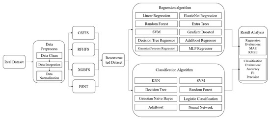
Figure 1.
Overall experimental process.
4.1. Experimental Setup
The computer used in this experiment has the following basic configuration: Windows 10 operating system, Intel(R) Core (TM) i7-8750 CPU @ 2.20 GHz, 8 GB RAM (Intel, Santa Clara, CA, USA). The experiment was conducted in Python 3.8. The training set and validation set were randomly partitioned with a ratio of 7:3.
To evaluate the performance of FSNT in feature selection for classification, three real datasets were chosen to assess the accuracy of classification, while another three real datasets were selected to examine the regression performance. The six real datasets used in the study are as follows: Student-por, Student-mat, Online News Popularity, Student Archive, Superconductivity, and TCGA Info with Grade; Student-por and Student-mat encompass scores of secondary school students from two Portuguese schools, collected through questionnaires and provided by [27]. Student-por is employed for regression to predict students’ final scores, which are continuous values, whereas Student-mat is utilized for classification to predict students’ scores divided into five categories. The Online News Popularity dataset, sourced from the website (www.mashable.com, accessed on 22 June 2023) and made available by [28], focuses on regression and aims to predict news popularity. Student Archive, provided by [29], was developed as part of a project to identify at-risk students early in their academic journey using machine learning technology; the dataset encompasses three types of classification tasks (dropout, enrollment, and graduates). The Superconductivity dataset, obtained from [30], pertains to superconducting materials and is used for regression to predict the critical temperature. TCGA Info with Grade involves the 20 most frequently mutated genes and three clinical features from projects. The objective is to determine whether patients exhibit specific clinical and molecular/mutation characteristics of LGG or GBM, as provided by [31]. These datasets are derived from practical applications and are typically employed to compare the classification performance of feature selection results in subsequent classification learning models, thereby evaluating the algorithm. Refer to Table 1 and Table 2 for basic information on these test datasets, including name, sample size, number of features, and number of categories.

Table 1.
Classified experimental datasets.
Table 2.
Regression experimental datasets.
To address the issue of data imbalance and ensure sample balance, we employed the SMOTENC algorithm [32]. This algorithm is an enhanced version of the SMOTE oversampling algorithm, and is capable of handling both continuous and discrete data. The algorithm’s workflow can be described as follows:
- (1)
- For each sample belonging to a minority class label, calculate its distance from sample points of other minority class labels in the multidimensional space. Obtain the k nearest neighboring points to the sample by performing the K-nearest neighbors (KNN) algorithm on the sample points of the minority class label.
- (2)
- Determine the sampling rate based on the proportion of each sample label type. For sample points belonging to a minority class with a relatively small proportion compared to other labels, randomly select a subset of samples from their k neighboring points. These selected samples are denoted as .
- (3)
- For continuous data, and each selected adjacent sample from the previous step, generate a new sample according to Equation (20):where represents a random number between 0 and 1, and .
- (4)
- For discrete data, the new sample value is determined by selecting the discrete value with the highest frequency of occurrence among the nearest neighbor samples.
4.2. Evaluation Metrics
To validate the effectiveness of the FSNT method, it is crucial to employ the information obtained through different feature reduction techniques as input for prediction models.
The performance improvement observed in prediction tasks after feature selection serves as evidence of the method’s effectiveness. Consequently, ten popular regression machine learning algorithms are utilized, namely: multiple linear regression [33], elastic net regression [34], random forest [35], extra trees [36], SVM [37], gradient boosted [38], decision tree regressor [39], AdaBoost regressor [40], Gaussian process regressor [41], and MLP regressor [42].
For classification tasks, eight machine learning algorithms are employed: KNN [43], SVM, decision tree, random forest, Gaussian naive Bayes [44], neural network [45], logistic algorithm [46], and AdaBoost [47]. To evaluate the regression performance, the following indicators are used:
- Mean absolute error (MAE)
This indicator is the expected value of absolute error loss
Root of square error or root of mean square error (RMSE), this indicator corresponds to the expectation of square (quadratic) error.
In order to evaluate the classification performance, the following indicators are used. In a binary classification problem where instances are classified into positive or negative classes, the classification process can result in the following four scenarios: (1) when an instance belongs to the positive class and is correctly predicted as positive, it is considered a true positive (TP); (2) if an instance is positive but is incorrectly predicted as negative, it is a false negative (FN); (3) if an instance is negative but is erroneously predicted as positive, it is a false positive (FP); (4) when an instance belongs to the negative class and is accurately predicted as negative, it is a true negative (TN).
Accuracy is defined as the ratio of the number of samples correctly classified by the classifier to the total number of samples in a given test dataset.
Precision is the ratio of the number of positive cases correctly classified to the number of instances classified as positive cases. It measures the accuracy of the algorithm.
To assess the strengths and weaknesses of various algorithms, the concept of the F1 score is introduced, which combines precision and recall to provide an overall evaluation; it integrates the outcomes of micro-average precision and micro-average recall, where 1 represents the optimal model output, while 0 represents the poorest model output:
In order to effectively measure the precision value for multiple classification targets, the micro-average precision is employed as the methodology. Firstly, the cumulative number of true positive (TP) and false positive (FP) predictions across all categories is computed. Subsequently, the precision and recall rate are calculated using these aggregated counts, as illustrated in Formula (26):
In addition to the aforementioned performance indicators, the effectiveness of data mining methods can also be evaluated by assessing the explained variance ratio. The explained variance ratio is defined as the ratio of the sum of variances of the selected features to the sum of variances of all features [48]. The calculation process is illustrated by the following formula:
where represents the total number of features reconstructed by feature selection, denotes the number of selected features, and represents the variance of the feature in the selected feature. A good feature selection method aims to achieve a high explanatory variance ratio while utilizing as few features as possible.
4.3. Analysis of Experimental Results of Classified Datasets with Different Feature Numbers
Figure 2 displays the average classification accuracy achieved by five feature selection algorithms (CSFFS, XGBFS, RFHFS, Baseline, and FSNT) along with eight classification algorithms (KNN, SVM, decision tree, random forest, Gaussian naive Bayes, neural network, logistic algorithm, and AdaBoost) on the Student Archive dataset. The x-axis represents the number of selected features (K), while the y-axis represents the average precision, average F1 score, and average accuracy obtained by each feature selection method. The black horizontal line represents the values obtained without using any feature selection algorithm. The comparison includes the FSNT algorithm and the three other feature selection algorithms, ranging from selecting 4 to 20 features.
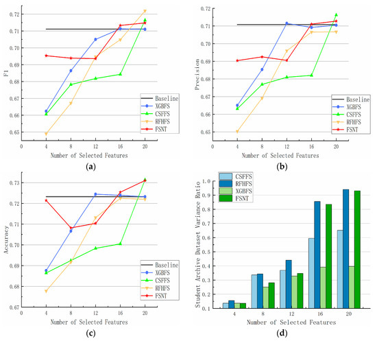
Figure 2.
Performance of different feature selection methods on Student Archive dataset. (a) F1; (b) precision; (c) accuracy; (d) dataset variance.
For the Student Archive dataset, the FSNT algorithm outperforms the other three algorithms in terms of F1 score, accuracy, and precision when k ≤ 8. It achieves the maximum values at k = 20, surpassing XGBFS in F1 score and slightly trailing behind the CSFFS method in precision. Moreover, the FSNT algorithm also outperforms other methods in accuracy.
Regarding the explanatory variance ratio chart for student achievement, the x-axis represents the number of selected features (k), while the y-axis represents the explanatory variance ratio obtained by each feature selection method. Both the CSFFS and FSNT methods exhibit significant superiority over the other two methods when k = 16. When the total number of features is 36, the FSNT method reaches a variance ratio exceeding 90% at k = 20, indicating the retention of the most information.
Figure 3 illustrates the feature selection algorithm ranging from 4 to 20 features. For the TCGA Info with Grade dataset, the FSNT algorithm initially falls behind the other three algorithms in terms of F1 score, accuracy, and precision from K ≥ 6 to 16. However, after k = 16, the FSNT method surpasses the CSFFS and RFHFS methods in F1 score, accuracy, and precision. At k = 20, all four methods exhibit similar performance across all evaluation criteria.
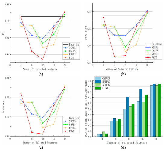
Figure 3.
Performance of different feature selection methods on TCGA Info with Grade dataset. (a) F1; (b) precision; (c) accuracy; (d) dataset variance.
On the explanatory variance ratio chart of the dataset, the CSFFS and FSNT methods outperform the other two methods when k = 8. Subsequently, the FSNT method begins to trail behind the CSFFS method until k = 20, while all methods maintain a variance ratio above 90%.
Figure 4 illustrates the feature selection algorithm ranging from 3 to 15 features. For the Student-mat dataset, the FSNT algorithm achieves its highest F1 score at k = 6 before decreasing. At k = 9 and k = 12, the FSNT algorithm performs slightly lower than the CSFFS method but significantly outperforms the XGBFS method. At k = 15, the FSNT algorithm, as Baseline, significantly surpasses the other three methods. In contrast, the XGBFS method consistently lags behind the other methods from k = 3 to k = 20. The RFHFS method initially decreases to its lowest value at k = 6, then gradually rises and approaches the performance of the CSFFS method. The CSFFS method consistently outperforms the XGBFS and RFHFS methods, reaching its peak at k = 9 and k = 12 before decreasing.
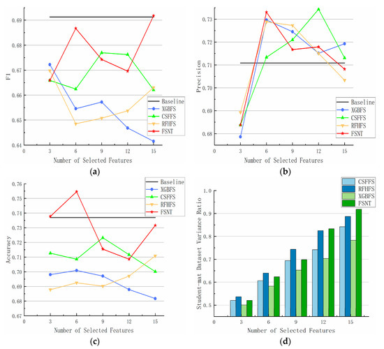
Figure 4.
Performance of different feature selection methods on Student-mat dataset. (a) F1; (b) precision; (c) accuracy; (d) dataset variance.
Regarding accuracy, all methods exhibit similar trends to the F1 score except for the FSNT method. The FSNT method achieves accuracy equivalent to Baseline at k = 3 and reaches its peak at k = 6, significantly surpassing the performance of the Baseline. For precision, except for the CSFFS method, all other methods peak at k = 6, significantly outperforming the performance of the Baseline, and then decrease. The CSFFS method reaches its peak at k = 12.
On the explanatory variance ratio chart of the dataset, the FSNT method outperforms the other three methods at k = 15, maintaining a unique variance ratio exceeding 90% and retaining the most information.
On the whole, the CSFFS, XGBFS, RFHFS, and FSNT algorithms demonstrate their respective advantages in classifying different datasets, although the RFHFS algorithm exhibits slightly inferior performance. However, the CSFFS algorithm solely selects features based on high correlation using the chi-square value, without considering feature differences or redundancy, resulting in poorer performance compared to information theory-based feature selection algorithms such as XGBFS, RFHFS, and FSNT. Based on the three evaluation criteria (F1, precision, and accuracy) for the three datasets and the explained variance ratio of the datasets, the classification accuracy of the FSNT method surpasses that of the CSFFS, XGBFS, and RFHFS methods. This indicates that the FSNT method is capable of generating feature subsets with stronger classification abilities.
4.4. Analysis of Experimental Results of Regression Datasets with Different Feature Numbers
Figure 5 illustrates the average regression accuracy obtained by four feature selection algorithms (CSFFS, XGBFS, RFHFS, and FSNT) and ten regression algorithms (multiple linear regression, elastic net regression, random forest, extra trees, SVM, gradient boosted, decision tree regression, AdaBoost regression, Gaussian process regression, and MLP regression) used on the Superconductivity dataset. The x-axis represents the number of selected features (K), while the y-axis represents the average MAE and average RMSE achieved by each feature selection method. The black horizontal line represents the Baseline. The FSNT algorithm and the other three feature selection algorithms were compared using feature subsets ranging from 6 features to 30 features.
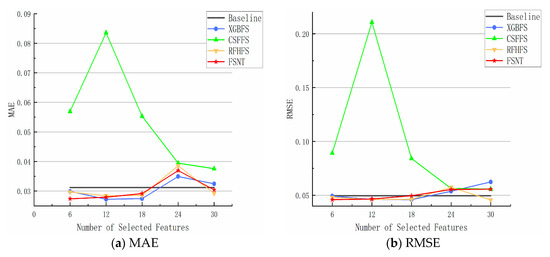
Figure 5.
Performance of different feature selection methods using different algorithms for Superconductivity datasets. (a) MAE; (b) RMSE.
On the Superconductivity dataset, the MAE and RMSE curves of XGBFS, RFHFS, and FSNT algorithms exhibit alternating increases with the number of selected features, whereas the MAE and RMSE curves of the CSFFS method initially rise and then decline, reaching their peak at k = 12, followed by a decrease with the increasing number of features. However, the final MAE and RMSE values for CSFFS are still larger than those of other methods. Regarding the MAE value, the XGBFS, RFHFS, and FSNT algorithms show slight increases as the number of features increases. When k ≤ 18, the three methods exhibit minimal differences compared to the MAE value of the Baseline and display horizontal oscillation. At k = 24, the maximum MAE value for the three algorithms surpasses the Baseline, after which it decreases. Finally, when k = 30, the three methods converge to the MAE value of the Baseline. Concerning the RMSE value, XGBFS, RFHFS, and FSNT algorithms demonstrate an alternating oscillation pattern below the horizontal line of the benchmark as the number of selected features increases. At k = 24, the RMSE value reaches its peak before decreasing. Only the RFHFS algorithm eventually matches the RMSE value of the Baseline, while the FSNT algorithm slightly surpasses RFHFS and XGBFS slightly surpasses FSNT.
As shown in Figure 6, on the Online News Popularity dataset, the MAE and RMSE values of the RFHFS and FSNT algorithms exhibit curves that remain below the curve obtained by the Baseline throughout the entire process. Additionally, at k = 18, these curves reach their lowest point before gradually increasing and returning to the horizontal line corresponding to the absence of feature selection at k = 30. In contrast, the MAE curve of the XGBFS algorithm oscillates around the horizontal line, reaching its peak at k = 18 and subsequently decreasing. Moreover, for k ≤ 12, its RMSE curve is lower than the curves of the other three algorithms, after which it gradually rises. At k = 18, it surpasses the RMSE curve of the RFHFS and FSNT algorithms, and, from k ≥ 24 onwards, the three curves converge. The CSFFS algorithm displays significant variation in its MAE and RMSE curves, continually rising until k ≤ 24. Notably, between k = 18 and k = 24, the curves experience a sharp increase, reach their maximum, and then decline. Finally, at k = 30, they return to the horizontal line representing the Baseline.
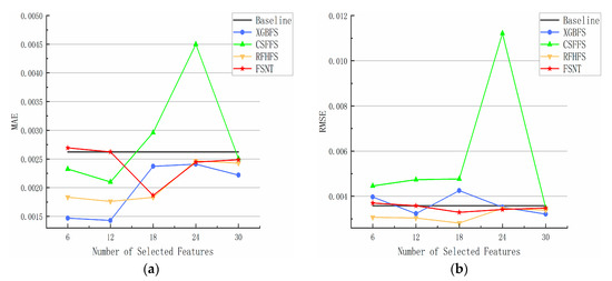
Figure 6.
Performance of different feature selection methods using different algorithms for Online News Popularity datasets. (a) MAE; (b) RMSE.
As shown in Figure 7, the FSNT algorithm and the other three feature selection algorithms involved in the comparison range from selecting 3 features to selecting 15 features. On the Student-por dataset, with the increase in feature selection number, the MAE and RMSE curves of the CSFFS, XGBFS, RFHFS, and FSNT feature selection algorithms show an alternating oscillation state, and the whole process is above the horizontal line. The MAE and RMSE curves of the XGBFS algorithm are generally below the curves of the other three algorithms, rising to the maximum MAE and RMSE at k = 9, and then falling to near the horizontal line. The MAE curve of the RFHFS algorithm reach the first peak at k = 6, reach the second peak at k = 12, and then continue to decline. The RMSE curve of RFHFS reaches the maximum at k = 6 and then decreases slowly until it rapidly decreases to the minimum at k = 30. The MAE curve of CSFFS is similar to the RMSE curve, reaching the maximum value at k = 6 and then decreasing slowly. Similarly, the MAE curve of the FSNT algorithm is similar to the RMSE curve. When k = 6, it drops to the lowest point, then rises to the highest point at k = 9, and then drops again. Finally, when k = 15, the three algorithms CSFFS, RFHFS, and FSNT descend to similar MAE and RMSE values.
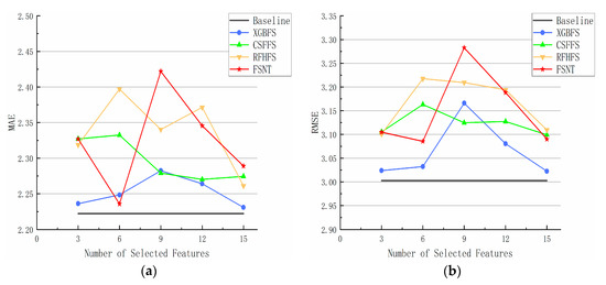
Figure 7.
Performance of different feature selection methods using different algorithms for Student-por datasets. (a) MAE; (b) RMSE.
Since the feature selection algorithm used for both the Student-por dataset and the Student-mat dataset selects the same features, and the explained variance ratio of the Student-mat dataset has been previously presented, there is no need to reiterate the explained variance ratio for the Student-por dataset.
As shown in Figure 8, Turning to the variance ratio of the Superconductivity dataset, the x-axis represents the number of selected features (k), while the y-axis represents the variance ratio obtained through the interpretation of each feature selection method. CSFFS, XGBFS, RFHFS, and FSNT all demonstrate an increase in variance ratio as the number of features increases. Among them, the RFHFS algorithm consistently yields the lowest variance ratio throughout the entire process, with the XGBFS algorithm also lagging behind the other two algorithms. Conversely, the CSFFS algorithm achieves the highest variance ratio. When the feature selection algorithm employs 81 features and k = 30, the explanatory variance ratio ranges between 0.7 and 0.8, indicating that it retains the most information. Similarly, when k = 30, the explanatory variance ratio of the FSNT algorithm surpasses 0.7, positioning it as the second-best method for information retention.
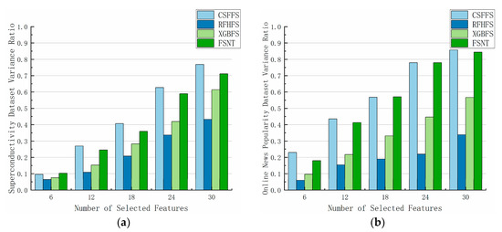
Figure 8.
Explanatory variance ratio of different feature selection methods on different datasets. (a) Superconductivity dataset variance; (b) Online News Popularity dataset variance.
Regarding the variance ratio of the Online News Popularity dataset, CSFFS, XGBFS, RFHFS, and FSNT exhibit an increase in variance ratio as the number of features increases. Throughout the entire process, the RFHFS algorithm consistently produces the lowest variance ratio, with the XGBFS algorithm also significantly trailing the other two algorithms. On the other hand, both the CSFFS and FSNT algorithms consistently maintain the same explanatory variance ratio, significantly surpassing the other algorithms. When the feature selection algorithm incorporates 61 features and k = 30, the explanatory variance ratio for both algorithms exceeds 0.8, meaning that, even with only 50% of the feature number used, more than 80% of the information is retained.
Overall, CSFFS, XGBFS, RFHFS, and FSNT exhibit distinct advantages in the classification results across different datasets, with RFHFS showing a slightly inferior performance. However, the CSFFS algorithm solely relies on selecting features based on high correlation according to the chi-square value, without considering feature differences or redundancy. Consequently, it performs worse compared to other feature selection algorithms based on information theory, such as XGBFS, RFHFS, and FSNT. When evaluating the three datasets using the two criteria of Mean Absolute Error (MAE) and Root Mean Squared Error (RMSE), along with considering the explained variance ratio, the classification accuracy of the FSNT method surpasses that of CSFFS, XGBFS, and RFHFS. This demonstrates that the FSNT method can obtain a feature subset with enhanced regression capabilities.
4.5. Analysis of Experimental Results of Different Datasets with Different Feature Selection Methods
In the classification evaluation, precision is chosen as the evaluation metric, indicating the proximity of the value to 1 corresponds to higher classification accuracy. The bold font in Table 3 represents instances where the precision value of FSNT is equal to or greater than that of other feature selection algorithms. The performance of four feature selection methods (CSFFS, XGBFS, RFHFS, and FSNT), along with a non-Baseline feature selection algorithm, is compared using eight classification algorithms. Across most datasets, once the number of features reaches 20, the explanatory variance ratio exceeds 90%. Further increasing the number of features does not result in a significant improvement in the explanatory variance ratio. Consequently, these feature selection methods all choose 20 features and their classification accuracy is compared in combination with different classifier ratios. This finding aligns with the analysis presented in literature [49].
Table 3.
Precision values of datasets based on different feature selection methods.
Table 3 presents the precision results of three datasets across eight classifiers: KNN, SVM, decision tree, random forest, Gaussian naive Bayes, neural network, logistic algorithm, and AdaBoost. The precision values in the table are reported with four decimal places. The bold values within each row indicate instances where FSNT outperforms the other three methods.
Regarding the Student-mat dataset in Table 3, FSNT achieves the highest precision value under the SVM classification algorithm, surpassing the other three feature selection algorithms by 5%. Conversely, under the logistic algorithm, CSFFS, XGBFS, RFHFS, and FSNT achieve the same optimal precision value, but it is 4.72% lower compared to the scenario without a feature selection algorithm. Additionally, when considering the Gaussian naive Bayes algorithm, the FSNT algorithm once again achieves the highest precision value, demonstrating the best classification accuracy among the student performance datasets. Notably, the FSNT algorithm outperforms the CSFFS algorithm by 2%, the XGBFS algorithm by 5.52%, the RFHFS algorithm by 1.02%, and the non-feature selection algorithm by 5.54%, showcasing its distinct advantages.
For the Student Archive dataset, the precision value of four of the eight classification algorithms for FSNT feature selection is the best. Among them, under the random forest and AdaBoost classification algorithms, the advantages of the FSNT algorithm are not obvious, but slightly better than CSFFS, XGBFS, and RFHFS. Under the decision tree classification algorithm, the notes algorithm is 1.57% higher than RFHFS, 1.56% higher than CSFFS, and 2.32% higher than XGBFS. Compared with other algorithms, the notes algorithm has advantages. Under Gaussian naive Bayes classification algorithm, the notes algorithm is 3.69% higher than RFHFS, 1.19% higher than CSFFS, and 1.87% higher than XGBFS. In the Student Archive dataset, the notes algorithm is significantly higher than the RFHFS algorithm, chi square filter, and XGBFS.
For the TCGA Info with Grade dataset, CSFFS, XGBFS, RFHFS, and FSNT achieved the same optimal precision under the SVM classification algorithm, logistic algorithm, and AdaBoost classification algorithm. Under the neural network classification algorithm, XGBFS and FSNT achieved the same optimal precision, slightly higher than RFHFS by 0.57% but significantly higher than CSFFS by 3.47%. In the decision tree classification, the precision obtained by FSNT is higher than that of the other three algorithms, which is significantly higher than that of the XGBFS algorithm by 2.99%, slightly higher than that of CSFFS and RFHFS, and also higher than the Baseline, with the best performance. In the TCGA Info with Grade dataset, the FSNT feature selection algorithm is not obvious but it still has advantages.
In general, the proposed FSNT algorithm performs better than other algorithms on average. Two of the three datasets have obvious advantages. The only algorithm competitive with the FSNT algorithm is the RFHFS algorithm. The experiment shows that the FSNT algorithm performs better in the student performance dataset and the Student Archive dataset than in the TCGA Info with Grade dataset. It can be concluded that the FSNT algorithm is more suitable for small sample datasets. In the student performance dataset, the highest classification precision value was 81.72%, which was determined by FSNT and Gaussian naive Bayes. In the Student Archive dataset, the highest classification precision value was 75.12%, which was determined by XGBFS and neural networks. In the TCGA Info with Grade dataset, the highest classification precision value was 89.24%, which was determined by FSNT and neural networks.
When using RMSE as the evaluation index for regression, a smaller difference between the predicted and real values indicates better performance. The bold font in Table 4 represents the RMSE values that are the same or smaller compared to FSNT and other feature selection algorithms. The performance of four feature selection methods, namely CSFFS, XGBFS, RFHFS, and FSNT, is compared with a feature selection algorithm not used as a Baseline, using 10 regression algorithms. In the dataset, when the number of features reaches 30, it can be observed from the above analysis that the explained variance ratio exceeds 80%. However, despite increasing the number of features, the explained variance ratio does not show significant improvement. Therefore, all these feature selection methods select 30 features.
Table 4.
RMSE values of datasets based on different feature selection methods.
Table 4 presents a summary of the RMSE values for the three datasets across 10 regression algorithms, which include linear regression, elastic net regression, random forest, extra trees, SVM, gradient boosted, decision tree regression, AdaBoost regression, Gaussian process regression, and MLP regression. The RMSE values are reported with four decimal places. The bold value in each row of the table indicates that FSNT achieves the same or better performance compared to the other three methods.
In Table 4, for the Student-por dataset, FSNT achieved the lowest RMSE under the elastic net regression algorithm, slightly surpassing the RMSE values of other feature selection algorithms and the Baseline by 1.3%. The FSNT algorithm exhibits a significantly lower RMSE value compared to CSFFS and RFHFS under the random forest regression algorithm, by 4.48%. The FSNT algorithm demonstrates superior regression performance compared to CSFFS and RFHFS by 2.57% under the SVM regression algorithm, and it also slightly outperforms RFHFS and the Baseline. The FSNT algorithm exhibits significant advantages under the decision tree regression algorithm. Its RMSE value is 14.13% lower than that of RFHFS, 10.77% lower than that of CSFFS, and 2.43% lower than that of XGBFS and the Baseline. The RMSE value of the FSNT algorithm remains the lowest among all feature selection algorithms under the Gaussian process regression algorithm, with a difference of approximately 2.8%.
For the student performance dataset, FSNT achieved the lowest RMSE under the elastic net regression algorithm, slightly surpassing the RMSE values of other feature selection algorithms and the Baseline by 1.3%. The FSNT algorithm exhibits a significantly lower RMSE value compared to CSFFS and RFHFS by 4.48% under the random forest regression algorithm. The FSNT algorithm demonstrates superior regression performance compared to CSFFS and RFHFS by 2.57% under the SVM regression algorithm, and it also slightly outperforms RFHFS and the Baseline. The FSNT algorithm exhibits significant advantages under the decision tree regression algorithm. Its RMSE value is 14.13% lower than that of RFHFS, 10.77% lower than that of CSFFS, and 2.43% lower than that of XGBFS and the Baseline. The RMSE value of the FSNT algorithm remains the lowest among all feature selection algorithms under the Gaussian process regression algorithm, with a difference of approximately 2.8%.
For the Online News Popularity dataset, the RMSE value of FSNT, along with the other three feature selection algorithms, is the same as the RMSE of the Baseline under the elastic net regression algorithm and SVM regression algorithm. The RMSE value of the FSNT algorithm is slightly lower than that of CSFFS, XGBFS, and RFHFS under the random forest regression algorithm. The FSNT algorithm demonstrates significant advantages under the AdaBoost regressor regression algorithm. Its RMSE value is 6.02% lower than RFHFS, slightly lower than CSFFS, and 14.35% lower than XGBFS and the Baseline. Among the three feature selection algorithms under the Gaussian process regression algorithm, the FSNT algorithm achieves the smallest RMSE value, which is approximately 13.72% lower than the Baseline.
In the Superconductivity dataset, the FSNT algorithm achieves an exceptionally low RMSE compared to other methods. The RMSE of FSNT is 0.0110, while CSFFS has an RMSE of 0.1062 and XGBFS has an RMSE of 0.1800, making FSNT only one-tenth of the magnitude of the other methods. Only RFHFS approaches the performance of FSNT, but the RMSE value of the Baseline is 0.0494, making FSNT 77.73% lower than the Baseline. Under the elastic net regression algorithm, the RMSE values of the four feature selection algorithms and the Baseline are the same value. Under the extra trees regression algorithm, FSNT achieves an RMSE value that is 8.16% lower than that of XGBFS, which is comparable to RFHFS, while CSFFS has a higher value than the Baseline. In the SVM regression algorithm, only FSNT and XGBFS have lower RMSE values than the Baseline, with FSNT having the lowest value. Under the MLP regressor regression algorithm, the RMSE value of the FSNT algorithm is significantly lower compared to CSFFS, XGBFS, and RFHFS, and it is the only algorithm with a lower value than the Baseline.
Overall, the proposed FSNT algorithm performs exceptionally well across all datasets and exhibits clear advantages. The RFHFS algorithm is the only competitor to the FSNT algorithm. The FSNT algorithm achieves an average reduction of 54.02% in the RMSE value for regression prediction by selecting the regression algorithm with the lowest RMSE in the dataset and averaging their results. The experiment demonstrates that the FSNT algorithm outperforms other algorithms in the regression dataset, suggesting its suitability for regression analysis.
5. Conclusions
Feature selection for high-dimensional data aims to maximize prediction accuracy by identifying the smallest possible subset of features. However, traditional methods suffer from drawbacks such as excessive parameter adjustments and significant variations in results among different classifiers. In this study, causality is introduced into the domain of feature selection. The FSNT algorithm is employed to identify causal relationships among features in high-dimensional datasets, constructing a causality diagram to guide the selection of features based on their causal strength. Three distinct feature selection algorithms, namely CSFFS, XGBFS, and RFHFS, are chosen, with the absence of a feature selection algorithm serving as the Baseline. The study employs six real-world datasets with varying sizes and domains, encompassing eight classification algorithms and ten regression algorithms.
The results indicate that the FSNT algorithm effectively eliminates redundant features in the three classification datasets and demonstrates superior overall classification performance compared to other feature selection algorithms. Among the three datasets, two datasets exhibit notable advantages, and the RFHFS algorithm emerges as the sole competitive algorithm to the FSNT algorithm. Across the three regression datasets, the FSNT algorithm performs exceptionally well and demonstrates clear advantages in regression evaluation for all datasets. The FSNT algorithm exhibits an average precision value improvement of 82.03% compared to other algorithms and achieves a significant reduction in the RMSE value. These results suggest that the FSNT algorithm is highly suitable for regression datasets. Extensive experiments have demonstrated the superior performance of the FSNT compared to other mainstream feature selection algorithms. However, it is observed that the running speed of the algorithm decreases when there is a large number of samples. Consequently, future research will focus on algorithm optimization and improving running speed to propose a more effective feature selection method.
Author Contributions
Conceptualization, J.L.; Methodology, J.L.; Validation, J.L.; Formal analysis, J.L.; Investigation, J.L.; Resources, J.L.; Data curation, J.L.; Writing—review & editing, G.Z.; Supervision, G.Z.; Project administration, H.W. All authors have read and agreed to the published version of the manuscript.
Funding
This work was supported by the National Natural Science Foundation of China (Grant Nos. 61263023 and 61863016).
Institutional Review Board Statement
Not applicable.
Informed Consent Statement
Not applicable.
Data Availability Statement
Data is presented in the article.
Conflicts of Interest
The authors declare no conflict of interest.
References
- Arcinas, M.M.; Sajja, G.S.; Asif, S.; Gour, S.; Okoronkwo, E.; Naved, M. Role of Data Mining in Education for Improving Students Performance for Social Change. Turk. J. Physiother. Rehabil. 2021, 32, 6519–6526. [Google Scholar]
- Puarungroj, W.; Boonsirisumpun, N.; Pongpatrakant, P.; Phromkhot, S. Application of data mining techniques for predicting student success in English exit exam. In Proceedings of the 12th International Conference on Ubiquitous Information Management and Communication, Langkawi, Malaysia, 5–7 January 2018; pp. 1–6. [Google Scholar]
- Batool, S.; Rashid, J.; Nisar, M.W.; Kim, J.; Mahmood, T.; Hussain, A. A random forest students’ performance prediction (rfspp) model based on students’ demographic features. In Proceedings of the Mohammad Ali Jinnah University International Conference on Computing (MAJICC), Karachi, Pakistan, 15–17 July 2021; pp. 1–4. [Google Scholar]
- Romero, C.; López, M.I.; Luna, J.M.; Ventura, S. Predicting students’ final performance from participation in on-line discussion forums. Comput. Educ. 2013, 68, 458–472. [Google Scholar] [CrossRef]
- Guyon, I.; Elisseeff, A. An introduction to variable and feature selection. J. Mach. Learn. Res. 2003, 3, 1157–1182. [Google Scholar]
- Aliferis, C.F.; Statnikov, A.; Tsamardinos, I.; Mani, S.; Koutsoukos, X.D. Local causal and markov blanket induction for causal discovery and feature selection for classification part II: Analysis and extensions. J. Mach. Learn. Res. 2010, 11, 235–284. [Google Scholar]
- Guang-yu, L.; Geng, H. The behavior analysis and achievement prediction research of college students based on XGBFS gradient lifting decision tree algorithm. In Proceedings of the 7th International Conference on Information and Education Technology, Aizu-Wakamatsu, Japan, 29–31 March 2019; pp. 289–294. [Google Scholar]
- Wang, C.; Chang, L.; Liu, T. Predicting Student Performance in Online Learning Using a Highly Efficient Gradient Boosting Decision Tree. In Proceedings of the International Conference on Intelligent Information Processing, Bucharest, Romania, 29–30 September 2022; Springer: Cham, Switzerland, 2022; pp. 508–521. [Google Scholar]
- Zheng, X.; Aragam, B.; Ravikumar, P.K.; Xing, E.P. Dags with no tears: Continuous optimization for structure learning. Adv. Neural Inf. Process. Syst. 2018, 31, 9472–9483. [Google Scholar]
- Yu, K.; Guo, X.; Liu, L.; Li, J.; Wang, H.; Ling, Z.; Wu, X. Causality-based Feature Selection: Methods and Evaluations. ACM Comput. Surv. 2020, 53, 1–36. [Google Scholar] [CrossRef]
- Venkatesh, B.; Anuradha, J. A review of feature selection and its methods. Cybern. Inf. Technol. 2019, 19, 3–26. [Google Scholar] [CrossRef]
- Spencer, R.; Thabtah, F.; Abdelhamid, N.; Thompson, M. Exploring feature selection and classification methods for predicting heart disease. Digit. Health 2020, 6, 2055207620914777. [Google Scholar] [CrossRef]
- Dufour, B.; Petrella, F.; Richez-Battesti, N. Understanding social impact assessment through public value theory: A comparative analysis on work integration social enterprises (WISEs) in France and Denmark. Work. Pap. 2020, 41, 112–138. [Google Scholar]
- Chen, T.; Guestrin, C. XGBFS: A Scalable Tree Boosting System. In Proceedings of the KDD ’16: 22nd ACM SIGKDD International Conference on Knowledge Discovery and Data Mining, San Francisco, CA, USA, 13–17 August 2016; pp. 785–794. [Google Scholar] [CrossRef]
- Ye-Zi, L.; Zhen-You, W.; Yi-Lu, Z.; Xiao-Zhuo, H. The Improvement and Application of Xgboost Method Based on the Bayesian Optimization. J. Guangdong Univ. Technol. 2018, 35, 23–28. [Google Scholar]
- Srivastava, A.K.; Pandey, A.S.; Houran, M.A.; Kumar, V.; Kumar, D.; Tripathi, S.M.; Gangatharan, S.; Elavarasan, R.M. A Day-Ahead Short-Term Load Forecasting Using M5P Machine Learning Algorithm along with Elitist Genetic Algorithm (EGA) and Random Forest-Based RFHFS Feature Selection. Energies 2023, 16, 867. [Google Scholar] [CrossRef]
- Chickering, D.M.; Meek, C.; Heckerman, D. Large-sample learning of bayesian networks is NP-hard. In Proceedings of the Nineteenth Conference on Uncertainty in Artificial Intelligence, Acapulco, Mexico, 7–10 August 2003; Morgan Kaufmann Publishers Inc.: Burlington, MA, USA, 2002. [Google Scholar] [CrossRef]
- Barber, D. Bayesian Reasoning and Machine Learning; Cambridge University Press: Cambridge, UK, 2012. [Google Scholar]
- Chickering, M. Optimal structure identification with greedy search. J. Mach. Learn. Res. 2003, 3, 507–554. [Google Scholar]
- Kalisch, M.; Bühlman, P. Estimating high-dimensional directed acyclic graphs with the PC-algorithm. J. Mach. Learn. Res. 2007, 8, 613–636. [Google Scholar]
- Shimizu, S. LiNGAM: Non-Gaussian methods for estimating causal structures. Behaviormetrika 2014, 41, 65–98. [Google Scholar] [CrossRef]
- Scheines, R.; Ramsey, J. Measurement error and causal discovery//CEUR workshop proceedings. NIH Public Access 2016, 1792, 1. [Google Scholar]
- Kang, D.G. Comparison of statistical methods and deterministic sensitivity studies for investigation on the influence of uncertainty parameters: Application to LBLOCA. Reliab. Eng. Syst. Saf. 2020, 203, 107082. [Google Scholar] [CrossRef]
- Janzing, D.; Balduzzi, D.; Grosse-Wentrup, M.; Schölkopf, B. Quantifying causal influences. Ann. Stat. 2013, 41, 2324–2358. [Google Scholar] [CrossRef]
- Liu, Y.; Bi, J.W.; Fan, Z.P. Multi-class sentiment classification: The experimental comparisons of feature selection and machine learning algorithms. Expert Syst. Appl. 2017, 80, 323–339. [Google Scholar] [CrossRef]
- Gao, W.; Hu, L.; Zhang, P. Feature selection by maximizing part mutual information. In Proceedings of the ACM International Conference Proceeding Series (ICPS), Shanghai, China, 28–30 November 2018. [Google Scholar] [CrossRef]
- Mansur, A.B.F.; Yusof, N. The Latent of Student Learning Analytic with K-mean Clustering for Student Behaviour Classification. J. Inf. Syst. Eng. Bus. Intell. 2018, 4, 156–161. [Google Scholar] [CrossRef]
- Zhang, Y.; Lin, K. Predicting and evaluating the online news popularity based on random forest. J. Phys. Conf. Ser. 2021, 1994, 012040. [Google Scholar] [CrossRef]
- Martins, M.V.; Tolledo, D.; Machado, J.; Baptista, L.M.; Realinho, V. Early Prediction of Student’s Performance in Higher Education: A Case Study. In Trends and Applications in Information Systems and Technologies: Volume 1 9; Springer International Publishing: Berlin/Heidelberg, Germany, 2021; pp. 166–175. [Google Scholar]
- Hamidieh, K. A data-driven statistical model for predicting the critical temperature of a superconductor. Comput. Mater. Sci. 2018, 154, 346–354. [Google Scholar] [CrossRef]
- Tasci, E.; Zhuge, Y.; Kaur, H.; Camphausen, K.; Krauze, A.V. Hierarchical Voting-Based Feature Selection and Ensemble Learning Model Scheme for Glioma Grading with Clinical and Molecular Characteristics. Int. J. Mol. Sci. 2022, 23, 14155. [Google Scholar] [CrossRef] [PubMed]
- Chawla, N.V.; Bowyer, K.W.; Hall, L.O.; Kegelmeyer, W.P. SMOTE: Synthetic minority over-sampling technique. J. Artif. Intell. Res. 2002, 16, 321–357. [Google Scholar] [CrossRef]
- Groß, J. Multiple Linear Regression; Springer Science & Business Media: Berlin/Heidelberg, Germany, 2003. [Google Scholar]
- Zou, H.; Hastie, T. Regularization and variable selection via the elastic net. J. R. Stat. Soc. Ser. B Stat. Methodol. 2005, 67, 301–320. [Google Scholar] [CrossRef]
- Breiman, L. Random Forests. Mach. Learn. 2001, 45, 5–32. [Google Scholar] [CrossRef]
- Geurts, P.; Ernst, D.; Wehenkel, L. Extremely randomized trees. Mach. Learn. 2006, 63, 3–42. [Google Scholar] [CrossRef]
- Xue, H.; Chen, S.; Yang, Q. Structural regularized support vector machine: A framework for structural large margin classifier. IEEE Trans. Neural Netw. 2011, 22, 573–587. [Google Scholar] [CrossRef]
- Zemel, R.S.; Pitassi, T. A Gradient-Based Boosting Algorithm for Regression Problems. In Neural Information Processing Systems; MIT Press: Cambridge, MA, USA, 2000. [Google Scholar]
- Xu, M.; Watanachaturaporn, P.; Varshney, P.K.; Arora, M.K. Decision tree regression for soft classification of remote sensing data. Remote Sens. Environ. Interdiscip. J. 2005, 97, 322–336. [Google Scholar] [CrossRef]
- Collins, M.; Schapire, R.E.; Singer, Y. Logistic regression, AdaBoost and Bregman distances. Mach. Learn. 2002, 48, 253–285. [Google Scholar] [CrossRef]
- Rasmussen, C.E.; Williams, C.K.I. Gaussian Processes for Machine Learning; MIT Press: Cambridge, MA, USA, 2006. [Google Scholar]
- Kashi, H.; Emamgholizadeh, S.; Ghorbani, H. Estimation of soil infiltration and cation exchange capacity based on multiple regression, ANN (RBF, MLP), and ANFIS models. Commun. Soil Sci. Plant Anal. 2014, 45, 1195–1213. [Google Scholar] [CrossRef]
- Zhang, M.L.; Zhou, Z.H. ML-KNN: A lazy learning approach to multi-label learning. Pattern Recognit. 2007, 40, 2038–2048. [Google Scholar] [CrossRef]
- Kesavaraj, G.; Sukumaran, S. A study on classification techniques in data mining. In Proceedings of the 2013 Fourth International Conference on Computing, Communications and Networking Technologies (ICCCNT), Tiruchengode, India, 4–6 July 2013. [Google Scholar]
- Saravanan, K.; Sasithra, S. Review on Classification Based on Artificial Neural Networks. Int. J. Ambient. Syst. Appl. 2014, 2, 11–18. [Google Scholar]
- Cheng, W.; Hüllermeier, E. Combining Instance-Based Learning and Logistic Regression for Multilabel Classification. Mach. Learn. 2009, 76, 211–225. [Google Scholar] [CrossRef]
- Schapire, R.E. Explaining adaboost. In Empirical Inference: Festschrift in Honor of Vladimir N. Vapnik; Springer: Berlin/Heidelberg, Germany, 2013; pp. 37–52. [Google Scholar]
- Gao, J.; Nuyttens, D.; Lootens, P.; He, Y.; Pieters, J.G. Recognising weeds in a maize crop using a random forest machine-learning algorithm and near-infrared snapshot mosaic hyperspectral imagery. Biosyst. Eng. 2018, 170, 39–50. [Google Scholar] [CrossRef]
- Ruangkanokmas, P.; Achalakul, T.; Akkarajitsakul, K. Deep Belief Networks with Feature Selection for Sentiment Classification. In Proceedings of the 2016 7th International Conference on Intelligent Systems, Modelling and Simulation (ISMS), Bangkok, Thailand, 25–27 January 2016. [Google Scholar] [CrossRef]
Disclaimer/Publisher’s Note: The statements, opinions and data contained in all publications are solely those of the individual author(s) and contributor(s) and not of MDPI and/or the editor(s). MDPI and/or the editor(s) disclaim responsibility for any injury to people or property resulting from any ideas, methods, instructions or products referred to in the content. |
© 2023 by the authors. Licensee MDPI, Basel, Switzerland. This article is an open access article distributed under the terms and conditions of the Creative Commons Attribution (CC BY) license (https://creativecommons.org/licenses/by/4.0/).