A Complex Network Important Node Identification Based on the KPDN Method

Abstract

In complex networks, identifying influential nodes is of great significance for their wide application. The proposed method integrates the correlation properties of local and global, and in terms of global features, the K-shell decomposition method of fusion degree is used to improve the actual discrimination degree of each node. In terms of local characteristics, the Solton index is introduced to effectively show the association relationship between each node and adjacent nodes. Through the analysis and comparison of multiple existing methods, it is found that the proposed method can identify key nodes more accurately so as to help quickly disintegrate the network. The final manual network verification also shows that this method is also suitable for the identification of important nodes of small-world networks and community networks.

1. Introduction

Many complex systems in the real world can be abstracted into models of complex networks [1,2]. In these complex systems, only a very small number of nodes are critical to the operation of the entire system. These nodes can be referred to as critical nodes because their activation or removal will significantly improve or reduce some functionality of the system. Finding the optimal set of key nodes in complex networks has been a long-standing problem in network science with many real-world applications. This is essential for apprehending suspects to stop terrorist activities [3], suppressing the spread of epidemics [4], controlling the spread of rumors [5], maintaining the stable operation of the network [6], and detecting and evaluating the vulnerability nodes of the network [7,8].

In recent years, many methods have been proposed to identify important nodes in networks, such as degree centrality (DC) [9], closeness centrality (CC), betweenness centrality (BC) [10], harmonic centrality (HC) [11], K-shell decomposition method (K-shell) [12], subgraph centrality (SC) [13], etc. In summary: (1) Existing methods face trade-offs between computational efficiency and identification accuracy. (2) Degree centrality and K-shell algorithms can roughly determine important nodes in networks, but are difficult to be accurate. (3) Betweenness centrality and harmonic centrality can judge node importance more accurately, but are difficult to apply to large-scale networks, and also face trade-offs. (4) Existing methods are difficult to achieve high efficiency and high precision at the same time.

At the same time, with the explosive growth of data in the information age today, the network connections in the real world are becoming more complex, and more methods for evaluating node importance are emerging. Morone and Makse [14] proposed a scalable theoretical framework called collective influence (CI) to identify a minimum set of key nodes. It is worth mentioning that CI has significant advantages over many previous algorithms in identifying node importance in maintaining network connectivity [15]. Meanwhile, the most common evaluation methods based on network position are the K-shell decomposition method [12] and its improved methods [16,17,18,19,20,21], which evaluate the importance of nodes by determining whether the nodes are in the central position of the network. The WL algorithm [22] is a sorting method based on node degree and neighbor node degree. This method relies heavily on local properties. The DWT algorithm [23] identifies isolated nodes with bridging functions based on local weak connections in the network and can determine the local properties of nodes more accurately. PageRank [24] is a node importance algorithm based on network topology. It calculates the global importance of nodes by simulating random walk processes and is significant for recommendation systems, web page ranking, etc. However, it relies solely on network topology without considering other attributes and cannot identify locally important nodes. INCC [25] is an improved method for detecting structural holes. Its advantage lies in its ability to identify structural holes in networks by relying on local connection patterns. Of course, this method has a strong dependence on the network topology. Existing literature indicates that INCC achieves suitable performance in analyzing propagation characteristics.

In recent years, some teams have also explored important node ranking methods using machine learning approaches [26]. These methods require constructing large datasets beforehand to train models for identifying important nodes in complex networks. It should be noted that the workload of data preparation and manual labeling is substantial in the early stages when using such methods. In addition, exploring important node identification in complex networks using machine learning approaches also has certain hardware requirements for the universal applicability of the models. Therefore, this study will continue to explore the properties of important nodes in complex networks along the line of traditional mathematics.

However, in practical applications, it is found that the above methods tend to focus on single local properties or global properties. For small-world networks or larger community networks, the effects of the above algorithms are not satisfactory. For more relevant node importance evaluation index methods, please refer to the review literature [27].

(1) There are various topological analysis methods for existing networks, but key node identification methods often focus on either local or global properties, and it is difficult to consider both simultaneously.

(2) Some analysis methods have high computational complexity, are unsuitable for large-scale networks, and require preset parameter threshold settings.

(3) The resolution of these methods is not high, and the ability to identify nodes in the network is insufficient.

The outline of this article is organized as follows. Section 2 introduces the proposed method and compares it with other algorithms. Section 3 introduces three metrics to evaluate the accuracy of importance ranking. Section 4 introduces 11 real complex networks and experimental data. Section 5 conducts simulation analysis on real and artificial networks and concludes with a summary in Section 6.

2. Materials and Methods

This article analyzes an undirected unweighted network $G\left(V,E\right)$ with $N=\left|V\right|$ nodes and $M=\left|E\right|$ edges. Let $A$ be the adjacency matrix of the network. If node $i$ is connected to node $j$, the element $a_{ij}$ of the adjacency matrix $A$ is 1; otherwise, it is 0. $k_i$ represents the degree of the node $i$, and $e_{ij}$ represents the edge between node and node $j$.

2.1. The Proposed Method

In response to the above problems, inspired by [20,23], this paper proposes a K-shell method positioned with degrees and neighbors (KPDN) and the KPDN method that combines the characteristics of degree, K-shell, and Solton [28]. Compared with traditional methods, this method comprehensively considers global and local network characteristics. It applies the K-shell method hierarchically on a global scale and records the isolation order in each layering process as the basis for secondary sorting. Finally, at the local level, it conducts a third round of sorting based on the relationship between each node’s degree value and adjacent nodes and the Solton index to distinguish node importance. Since the KPDN method does not contain free parameters and each calculation step is recorded along with the K-shell expansion process, it does not require pre-computation of parameter values, reducing computational overhead and complexity. The specific steps are as follows:

The improved fused degree K-shell method (recording the peeling order of each node under each shell layer while comparing degree values of the same peeling order).

First, use K-shell to record which K-shell layer each node belongs to. Second, when nodes in the same K-shell layer are peeled off sequentially, record the order in which the node is peeled off as well as the layer number and sequence number. Finally, in each set of nodes with the same layer and peeling order, sort in descending order according to the proportion of node degree values. The calculation steps are as follows.

Step 1: Inspired by the literature [20], we construct a new formula to calculate important nodes, calculate the peeling order of nodes under the same shell layer, and mark the nodes. To first record the peeling order of nodes under the same shell layer, the formula is as follows:

$$KS{L}_{k{s}_i,l_i}=\frac{l_i}{l_{\max }+1}MAX\left(1, k{s}_{i|next}-k{s}_i\right)$$

(1)

where $k{s}_i$ is the $k\text{-}shell$ value of node $i$, $l_i$ is the peeling order of node $i$ under the same $k{s}_i$ shell iteration peeling operation, and $l_{\max }$ is the maximum peeling order number under the same shell layer; $k{s}_{i|next}$ is the $k\text{-}shell$ value adjacent to node $i$, and when node $i$ is at the maximum $k\text{-}shell$ layer, the $k{s}_{i|next}-k{s}_i$ value is automatically set to 1. Where KSL is (K-shell methods with layers).

Step 2: We summarize the nodes under the same peeling order layer (i.e., the same value) in the same shell layer (i.e., the same value) and sort them in descending order of the current degree values of each node. Where KPD is (K-shell methods positioned with degrees). The formula is as follows:

$$KP{D}_i=k{s}_i+k_i+\frac{k_i}{k_{N(i)\max }+1}KS{L}_{k{s}_i,l_i}$$

(2)

where $k_i$ is the degree value of node $i$, $k_{N(i)\max }$ is the maximum degree value of the neighboring nodes of node $i$, and $k{s}_i$ is the $k\text{-}shell$ value of node $i$, the same as above.

Step 3: Inspired by the literature [23,24,25], we calculate the adjacent nodes of each obtained node. Here, inspired by previous research, we define the edge intensity between two connected nodes based on the local information of network topology, such as the Solton index proposed in [23,24,25]: The formula is as follows:

$$S_{ij}=\frac{\left|N\left(i\right)\cap N\left(j\right)\right|}{\left|N\left(i\right)\cup N\left(j\right)\right|}$$

(3)

Of course, in the actual debugging process, we found that replacing the denominator (4) with this method produced slightly better results.

$$S_{ij}=\frac{\left|N\left(i\right)\cap N\left(j\right)\right|}{\sqrt{k_i\ast k_j}}$$

(4)

where $N\left(i\right)$ and $N\left(j\right)$ are the set of adjacent nodes of nodes i and j, respectively.

The above operations can form an initial dictionary during the first traversal of the K-shell and store it, and constantly call it to save computation time. We incorporate this indicator into the KPD method:

$$KPD{N}_i={\displaystyle \sum _{j\in N\left(i\right)}{\left(\frac{S_{ij}+k_i}{KP{D}_j}\right)}^2}$$

(5)

In summary, the above operations can form an initial dictionary during the first traversal of K-shell for storage and constantly call to save calculation time. Therefore, from a theoretical analysis, the computational complexity of the proposed method in this paper should be close to the K-shell method. Therefore, it is determined that this method is more suitable for large-scale networks. The KPDN method is shown in Figure 1.

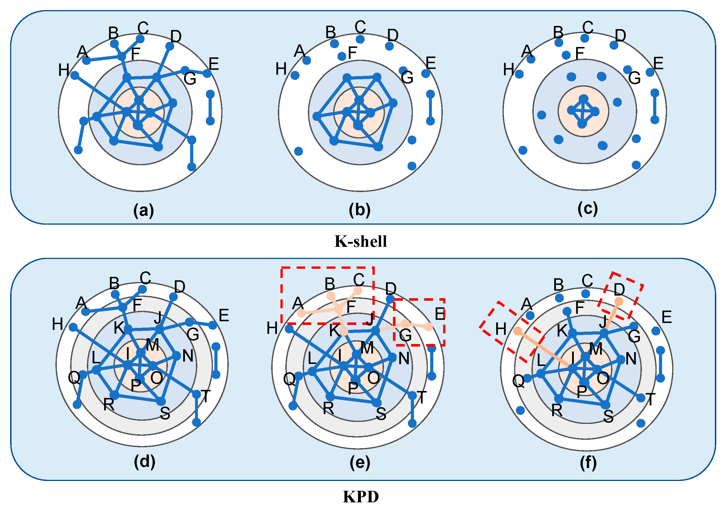
The traditional K-shell method divides the levels of complex networks roughly. As shown in Figure 2a–c, nodes A, B, C, D, E, F, G, and H are at the same 1-shell level, and the importance of nodes is not further distinguished. However, in the KPD method, we record the order of peeling off at the same 1-shell level synchronously during the decomposition process. For example, nodes A, B, C, D, E, and H are the first nodes peeled off in the 1-shell, marked as $l_A=l_B=l_C=l_D=l_E=l_H=1$. Nodes G and F are the second nodes peeled off in the 1-shell layer, marked as $l_G=l_F=2$. Because the 1-shell layer is peeled off twice in total, $l_{\max }=2$. At the same time, because the neighboring nodes of each node are different, as shown in Figure 2e,f, the neighboring nodes of nodes A, B, and C only have F, while the neighboring node of node H is I, and the neighboring node of node D is J. Therefore, the maximum K-shell values of the neighboring nodes of each point are different, with values of $k{s}_{A|next}=k{s}_{B|next}=k{s}_{C|next}=1$, $k{s}_{D|next}=3$, $k{s}_{H|next}=3$, $k{s}_{G|next}=k{s}_{F|next}=3$, respectively. Similarly, the maximum degree values of the neighboring nodes of each point can be obtained: $k_{N(D)\max }=5$, $k_{N(H)\max }=6$, $k_{N(A)\max }=k_{N(B)\max }=k_{N(C)\max }=k_{N(E)\max }=2$, $k_{N(G)\max }=5$, $k_{N(F)\max }=4$.

Plugging the above parameters into Formula (2) yields the following values from A to H are as follows:

$$KP{D}_H\approx 2.0952,KP{D}_A=KP{D}_B=KP{D}_C=KP{D}_E\approx 2.1111,KP{D}_D\approx 2.1666$$

$$KP{D}_G\approx 3.4444,KP{D}_F\approx 5.5333.$$

Through the KPD method, we can further distinguish the importance of nodes within the same K-shell layer. The importance of nodes F and G is higher than that of D and H, and also, the importance of nodes D and H is higher than that of A, B, C, and E. This shows that the KPD method can more accurately identify the topological structure of complex networks and effectively correct the deficiencies of the traditional K-shell method.

Then we demonstrate calculating the KPDN value of node K. First, traversing the neighbor nodes of node k forms the $\mathrm{\Gamma }(K)=\{F,J,M,L\}$. Since there are 4 nodes adjacent to k, we need to calculate $S_{KF},S_{KJ},S_{KM},S_{KL}$, a total of 4 Solton index values. The results are as follows: First, calculate $S_{KF}$.

To compute $S_{KF}$, we first need to traverse the neighbor sets of nodes K and F. The neighbor set of K is: $\mathrm{\Gamma }(K)=\{F,J,M,L\}$, and the neighbor set of F is: $\mathrm{\Gamma }(F)=\{A,B,C,K\}$. Then, we perform the “and” operation on the two sets and plug them into Formula (4) to obtain $S_{KF}=0$.

Similarly, to compute the value of S2, the neighbor sets of nodes K and J are $\mathrm{\Gamma }(K)=\{F,J,M,L\}$ and $\mathrm{\Gamma }(J)=\{D,K,M,N,G\}$ respectively. Subsequently, plugging them into Formula (4) yields $S_{KJ}=\frac{1}{\sqrt{4\ast 5}}=\frac{\sqrt{5}}{10}$.

And also, calculating $S_{KM}=\frac{\sqrt{5}}{10}$, $S_{KL}=0$.

The degree of node K is: $k_K=4$,

The KPD value of node K is: $KP{D}_K\approx 7.2222$,

Plugging the above parameters into Formula (5) yields: $KPD{N}_K\approx 0.1441655$.

Based on the node sorting values generated by different algorithms, after deleting the nodes ranked in the top 40%, respectively, the largest connected subgraph of the remaining nodes was annotated and compared, and the largest connected subgraph in each figure was marked in red for easy identification, as shown in Figure 3.

As shown in Figure 3, a randomly generated small-world network with 100 nodes is used. Nodes are sorted using the CI method, degree method, and KPDN method, respectively. After removing the top 40% of nodes from each method, the maximum connected components of the remaining networks are 52%, 47%, and 24% of the size of the original network, respectively.

2.2. The Existing Benchmark Methods

In this paper, we use several well-known metrics to study the performance of the proposed method. These measures include:

1.

Degree centrality (DC)

Degree centrality is a basic ranking algorithm for identifying node importance. The degree of node i is defined as follows:

$$k_i={\displaystyle \sum _{j=1}^N{a}_{ij}}$$

(6)

2.

Collective influence (CI)

The collective influence of a node is defined as follows:

$$C{I}_i=\left(k_i-1\right){\displaystyle \sum _{j\in set(i,l)}\left(k_j-1\right)}$$

(7)

3.

Betweenness centrality (BC)

Betweenness centrality refers to the number of times a node appears in all shortest paths in a graph, that is, the importance of the node in connecting other nodes in the network. It is defined as follows:

$$B{C}_i={\displaystyle \sum _{i\in d{\left(i,j\right)}_{\min },i\ne j}1}$$

(8)

4.

K-shell decomposition method

The K-shell decomposition method proposed by Kitsak et al. [19,20,21] is a graph-theoretical algorithm used to decompose an undirected graph into multiple K-shell subgraphs. A K-shell subgraph refers to a subgraph composed of nodes with degrees greater than or equal to k in the graph; that is, any node in the subgraph has a degree greater than or equal to k. The core idea of the algorithm is to repeatedly prune the nodes with the smallest degrees and update the degrees of their adjacent nodes until all nodes are decomposed into K-shell subgraphs.

5.

WL algorithm

The WL algorithm [22] is a ranking method based on node degree and adjacent node degree. It is defined as follows:

$$W{L}_i={\displaystyle \sum _{j\in N\left(i\right)}\left(k_i\times k_j\right)}$$

(9)

6.

DWT algorithm

The DWT algorithm is a decomposition method proposed by Yirun Ruan et al. [23]. It quantifies the strength of links based on local information of network topology and designs a simple and effective method to evaluate the importance of nodes according to the number of connections and overlap of neighbors.

$$DW{T}_i={{\displaystyle \sum _{j\in N\left(i\right)}\left(\raisebox{1ex}{$1$}\!\left/ \!\raisebox{-1ex}{$k_i$}\right.+\raisebox{1ex}{$S_{ij}$}\!\left/ \!\raisebox{-1ex}{$k_i$}\right.\right)}}^2,S_{ij}=\frac{\left|N\left(i\right)\cap N\left(j\right)\right|}{\sqrt{k_i\times k_j}}$$

(10)

7.

Harmonic centrality

The harmonic centrality (HC) method is defined as follows:

$$H{C}_i={\displaystyle \sum _{j\ne i}\frac{1}{d\left(i,j\right)}}$$

(11)

8.

Closeness centrality

Closeness centrality (CC) is a node centrality measurement method used to measure the distance from a node to other nodes, that is, its average shortest path length to other nodes. It is defined as follows:

$$C{C}_i=\frac{1}{n}{\displaystyle \sum _{j\ne i}d\left(i,j\right)}$$

(12)

9.

Pagerank

PageRank [24] is an algorithm proposed by Page and Brin, the co-founders of Google, to rank web pages. The specific formula is as follows:

$$PR\left(i\right)=\frac{\left(1-d\right)}{n}+d\ast {\displaystyle \sum _{j\in \mathrm{\Gamma }\left(i\right)}\frac{PR\left(j\right)}{C\left(j\right)}}$$

where $PR\left(i\right)$, $PR\left(j\right)$ represent the PageRank values of nodes $i$ and $j$, $C\left(j\right)$ represents the outdegree of the node, $d$ is the damping factor, usually 0.85, $n$ is the total number of web pages, and $\mathrm{\Gamma }\left(i\right)$ is the set of neighboring nodes of node $i$.

10.

INCC

The INCC method [25] combines the direct and indirect influences of a node’s nearest neighbors and next-nearest neighbors. The specific formula is as follows:

$$INC{C}_i={{\displaystyle \sum _{j\in \mathrm{\Gamma }(i)}\left(p_{ij}^{\prime }+{\displaystyle \sum _{k=1,k\ne i,j}^n{p}_{ik}^{\prime }{p}_{kj}^{\prime }}\right)}}^2$$

where $p_{ij}^{\prime }=\frac{Q_i}{L{R}_i}$, $L{R}_i={\displaystyle \sum _{j\in \mathrm{\Gamma }(i)}{Q}_i}$, $Q_j={\displaystyle \sum _{w\in \mathrm{\Gamma }(j)}{N}_w}$, $N_w$ represent the sum of the degrees of the two-step neighbors of node $w$; $\mathrm{\Gamma }(i)$ and $\mathrm{\Gamma }(j)$ represent the sets of neighbors of nodes $i$ and $j$, respectively.

11.

Randomness method

Rank the importance of network nodes by random scoring.

3. Evaluation Index

3.1. Maximum Connectivity Coefficient

The maximum connectedness coefficient is another metric for evaluating the performance of ranking methods. It is defined as follows:

$$P_{Subnet}=\frac{R}{N}$$

(13)

where $R$ is the size of the largest connected subgraph after removing the node, and $N$ represents the size of the original connected network. Therefore, the smaller the $P_{Nodes}$ value, the smaller the proportion of the largest connected subgraph after removing the node from the original graph, which proves the better effect of removing the node.

3.2. Average Remaining Edges of the Network

The remaining edges of the network are an important metric that allows us to better realize the remaining connectivity of the network after a node is destroyed. It can be used not only for subsequent path analysis but also as an important indicator of the network repair cost. It is calculated as follows:

$$P_{Edges}=\frac{E}{M}$$

(14)

where $E$ is the total number of edges remaining in the network after removing nodes each time, and $M$ is the number of edges in the initial network.

3.3. Network Sensitivity

The network sensitivity is calculated as follows:

$$S={\displaystyle \sum _{s<\sigma }\frac{n_s{s}^2}{n}}$$

(15)

where $n_s$ is the number of components of size $s$, $n$ is the number of network nodes, and $\sigma$ is the threshold for remaining fragments to determine whether the network is destroyed. As network nodes are gradually removed, the network is decomposed into many small disconnected parts, that is, small network fragments. When the network disintegrates to a certain extent, there is often a peak sensitivity $S$ in the image, and the peak also means that the original network has been maximally decomposed into fragment groups less than or equal to the threshold $\sigma$.

3.4. Network Monotonicity

The network sensitivity is calculated as follows:

A suitable node importance ranking algorithm should assign each node a unique ranking index. If there are multiple nodes at the same ranking index, such an algorithm is considered in need of improvement. To quantitatively measure the resolution of different methods, the monotonicity indicator M(R) of the ranking list is used.

$$M\left(R\right)={\left[1-\frac{{\displaystyle {\sum }_{r\in R}L\ast \left(L-1\right)}}{n}\right]}^2$$

(16)

where $L$ is the number of nodes with the same index value. If $M\left(R\right)=1$, it indicates that the algorithm is perfectly monotonic (with each node classified into a different index value), whereas $M\left(R\right)=0$ means all nodes are classified into the same score (or rank). The monotonicity indicator reflects whether the ranking algorithm can well distinguish nodes, i.e., the resolution of nodes.

4. Datasets

To demonstrate the influence of different node deletion strategies on networks with different scales, we selected six real networks with sizes ranging from ${10}^3$ to ${10}^4$, and five real networks with sizes ranging from ${10}^4$ to ${10}^5$, as shown below:

The detailed information on the datasets is shown in

Table 1. Relevant parameters of real networks (${10}^3–{10}^4$ ).

Dataset	N	M	<k>	Density	Clustering
email-univ	1133	5451	4.811120918	0.43%	22.02%
power-eris1176	1176	9864	8.387755102	0.71%	43.20%
fb-pages-government	7057	89,455	12.67606632	0.18%	41.09%
US-airports	1574	17,215	10.93710292	0.70%	50.42%
bio-grid-worm	3507	6531	1.8622754	0.05%	4.88%
p2p-Gnutella08	6301	20,777	3.297413109	0.05%	1.09%

and

Table 2. Relevant parameters of real networks (${10}^4–{10}^5$ ).

Dataset	N	M	<k>	Density	Clustering
dimacs10-astro-ph	16,046	121,251	7.55646267	0.05%	66.51%
ca-Astroph	18,771	198,050	10.55084971	0.06%	63.06%
gottron-reuters	38,677	978,174	25.29084469	0.07%	4.73%
prosper-loans	89,269	3,330,022	37.30322956	0.04%	0.49%
facebook-wosn-links	63,731	817,035	12.82005617	0.02%	22.10%

.

4.1. Networks with Scale ${10}^3–{10}^4$

(1) email-univ. The email-univ dataset from SNAP is an email communication network containing 1133 nodes and 5451 edges. Nodes represent university employees, and edges indicate communication between employees. This dataset is often used for social network analysis, with the feature of a high average clustering coefficient.

(2) US-airports. The US-airports dataset from SNAP represents the airline network between airports in the United States, containing 1574 airport nodes and 17,215 airline edges. This dataset can be used for transportation network analysis, with a relatively small average shortest path length.

(3) power-eris1176. The power-eris1176 dataset from KONECT is a power grid network containing 1176 power station nodes and 9864 power supply edges. This dataset is used for power grid modeling and analysis, with a small network diameter.

(4) bio-grid-worm. The bio-grid-worm dataset contains 3507 protein nodes and 6531 functional association edges from the protein–protein interaction network of the nematode Caenorhabditis elegans in the BioGRID database. This dataset is applied in bioinformatics network analysis with high network density.

(5) p2p-Gnutella08. The p2p-Gnutella08 dataset from SNAP is a P2P file-sharing network containing 6301 user nodes and 20,777 file transfer edges. This dataset is used for P2P network modeling, with a relatively high clustering coefficient.

(6) fb-pages-government. The fb-pages-government dataset from SNAP is a Facebook page network containing 7057 government organization page nodes and 89,455 inter-page edges. This dataset is often used for social network analysis, with a small network diameter and large clustering coefficient.

4.2. Networks with Scale ${10}^4–{10}^5$

(1) dimacs10-astro-ph. The dimacs10-astro-ph dataset from the DIMACS challenge is a co-authorship network in the field of astrophysics. This dataset contains 16,046 author nodes and 121,251 collaboration edges between them. It can be used to analyze the structural characteristics of academic collaboration networks, with the features of low network density but a high average clustering coefficient.

(2) ca-Astroph. The ca-Astroph dataset is extracted from the arXiv e-print repository for the astrophysics collaboration network. The dataset scale is similar to dimacs10-astro-ph, containing 18,771 author nodes and 198,050 collaboration edges. This dataset is often used for academic collaboration network analysis, with a distinct core-periphery structure.

(3) gottron-reuters. The gottron-reuters dataset built by Gottron et al. is a Reuters news text network containing 38,677 news article nodes. Edges are constructed between pairs of topically similar articles, with a total of 978,174 edges. This dataset can be used for text network analysis with high modularity.

(4) prosper-loans. The prosper-loans dataset from the Prosper lending website contains 89,269 borrower nodes and 3,330,022 lending relationship edges between them. This is a typical financial transaction network dataset, often used for complex network analysis, with scale-free degree distribution.

(5) facebook-wosn-links. The facebook-wosn-links dataset represents the linkage network between different Facebook pages, containing 63,731 page nodes and 817,035 inter-page linkage edges. This dataset can be used for social network analysis, with a high clustering coefficient and obvious community structure.

As well as three artificial datasets: watts-strogatz [29], LFR [30], and barabasi-albert [31].

5. Results and Analysis

5.1. Analysis of Real Networks

5.1.1. Size of Real Network from ${10}^3$ to ${10}^4$

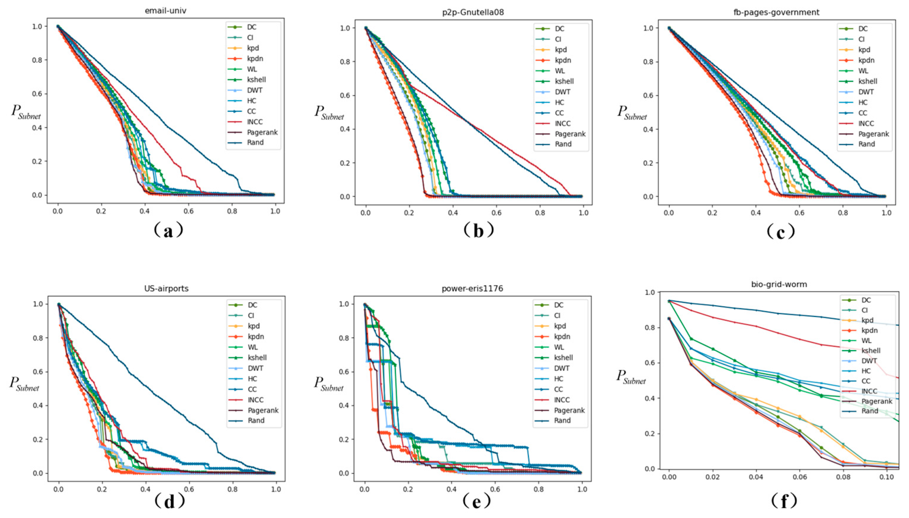
As shown in Figure 4, this section compares the performance of the proposed method with other methods in actual networks. The robustness of networks under node removal was studied. In most cases, the proposed method outperforms other methods, and the relative size of the largest connected subgraph decreases faster.

For example, Figure 4b shows the comparison of the decrease rate of the largest connected subgraph after deleting 20% of nodes in the source network by different methods. The results are: KPDN: 36.75%, PageRank: 37.82%, DWT: 54.31%, Degree: 58.88%, KPD: 62.06%, WL: 63.88%, CI: 64.16%, CC: 67.06%, K-shell: 68.31%, INCC: 67.44%, Random: 75.06%. Similarly, as shown in Figure 4a–e, the effect of deleting nodes on the connectivity coefficient of subnets is the most obvious. And, the effect is slightly better than other methods.

Therefore, the method in this paper (the red curve in Figure 4) surpasses other methods in most cases, and the relative scale of the largest connected subgraph decreases more significantly. At the same time, it should be noted that in the comparison curves of each method, the relative scale of the largest connected subgraph does not decrease with the removal of nodes. For example, the power-eris1176 and bio-grid-worm datasets in Figure 4e,f. This is mainly because the initial node sorting method continues to change with the removal of the first batch of sorted nodes. The remaining network structure is different from the initial node importance sorting.

We not only intuitively compare the size of the largest connected subgraph of the remaining subgraph but also introduce three indicators: subgraph sensitivity index, subgraph network connectivity efficiency, and number of remaining edges in the subgraph for supplementation.

The threshold set in this paper is 100% of the original network size. When the susceptibility index peaks after removing a certain percentage of nodes, it means that each method has maximally decomposed the original network into fragments below the threshold size. Then, as the fragments continue to shrink, the susceptibility enters a downward stage. It can be observed from Figure 5 that the proposed method in this paper has an obvious effect on the change in the susceptibility index of the subgraph.

To further demonstrate the sensitivity results on these six real-world networks of scale from ${10}^3$ to ${10}^4$, we have summarized the node consumption ratio when each real-world network reaches the extreme point under different removal strategies.

Taking Figure 5b as an example, when the peak appears, the proportion of nodes removed is: KPDN: 11.46%, PageRank: 12.94%, DWT: 18.81%, Degree: 18.83%, KPD: 22.05%, INCC: 22.16%, CI: 22.46%, WL: 22.91%, K-shell: 24.33%, HC: 24.20%, CC: 24.43%, Random: 24.81%. Similarly, in Figure 5b,c,f, it can be seen that the network can be quickly fragmented by deleting fewer nodes. At the same time, it can also be observed from Figure 5a,d,e that the proposed method is in a leading position. Therefore, the proposed method in this paper has an obvious effect on the change in the susceptibility index of the subgraph.

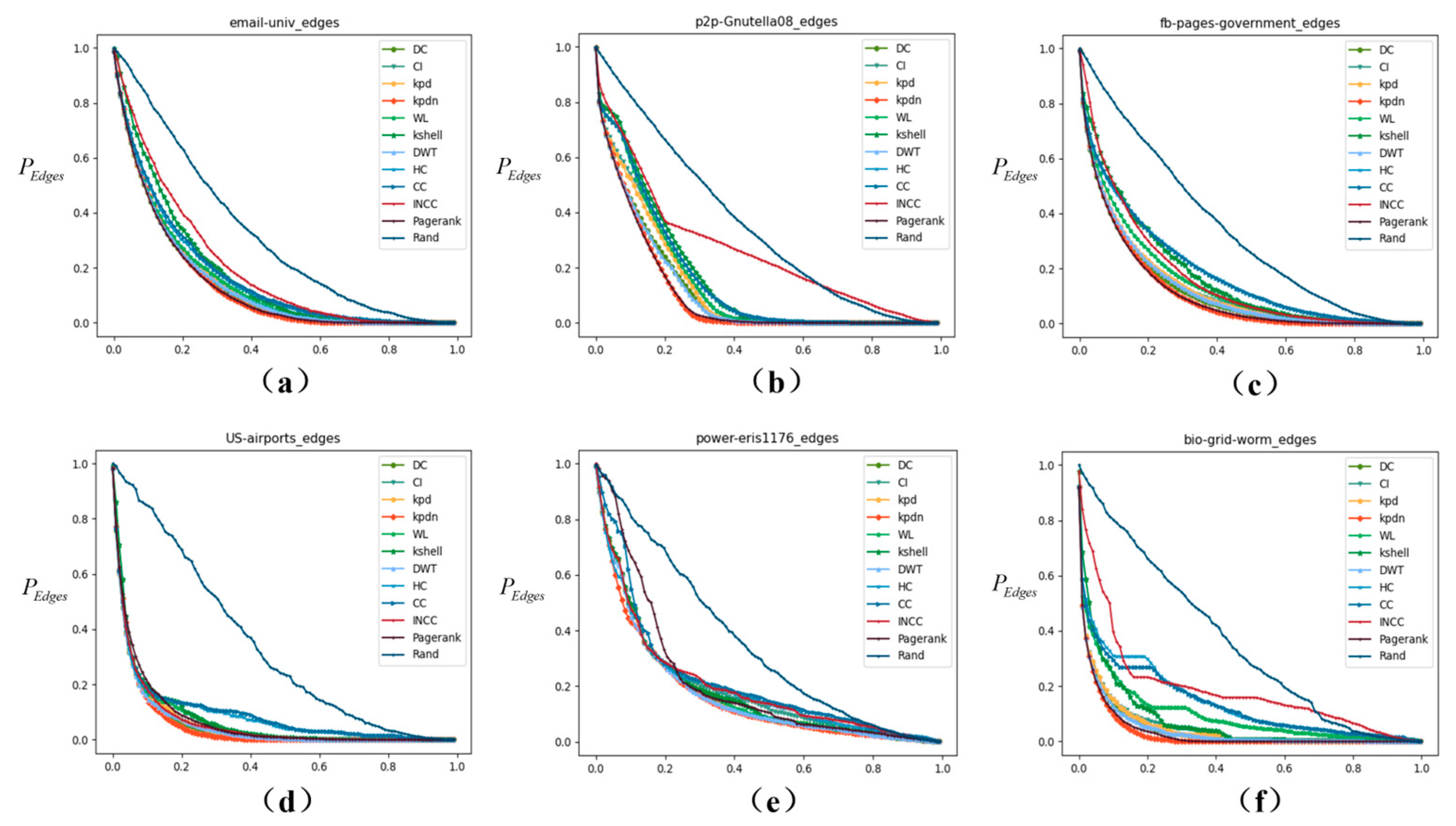
It can be observed from Figure 6 that the impact of network node removal on the remaining number of network edges varies with different networks. For example, in air transport networks, as some airports are gradually removed due to weather and other factors, the air routes related to the removed nodes will also be affected and canceled. Therefore, the remaining number of network edges is also an important indicator. According to the actual data, it can be observed from Figure 6 that the proposed method in this paper has an obvious effect on the change in the edge residual rate index of the subgraph. Taking Figure 6c as an example, When 20% of the nodes in the original network are deleted, the calculation results are: KPDN: 19.6875%, PageRank: 19.8865%, Degree: 21.10%, DWT: 21.72%, KPD: 22.34%, WL: 26.69%, INCC: 38.67%, K-shell: 33.88%, CC: 34.94%, Random: 62.51%, CI: 96.13%. Similarly, it can be seen that the effects of Figure 6a–d,f are quite ideal, and the effect of Figure 6e is also slightly better.

5.1.2. Size of Real Network from ${10}^4$ to ${10}^5$

Due to the discovery in the experimental process that for large network node attack experiments, the efficiency of centrality evaluation indicators based on path analysis is very low, so when analyzing networks of ${10}^4\sim {10}^5$ this scale, we will no longer participate in BC, HC, CC, and CI comparison experiments to balance the overall experiment efficiency (we will also continue to retain the BC, HC, CC, and CI methods in the original code so that interested readers can verify and try for themselves).

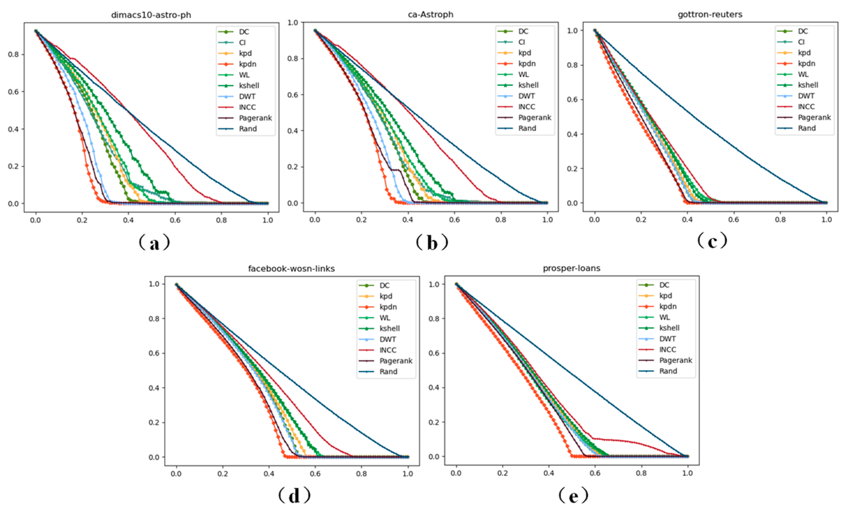
From Figure 7, it can be clearly seen that on the newly added network data of scale ${10}^4\sim {10}^5$, the KPDN method proposed in this paper can achieve suitable results in terms of the largest connected component size, meaning the method proposed in this paper has strong robustness in node removal. Meanwhile, in order to describe the actual data of each point in more detail, we show the data under different thresholds in Table S1 of Supplementary File S3.

As can be seen more clearly from Figure 7, the method proposed in this paper has achieved suitable performance on the five existing real-world datasets of scale ${10}^4\sim {10}^5$. (Note: 0% in the tables refers to the actual removal effect when the top 1 ranked node is removed according to different strategies).

From Figure 8, it can be clearly seen that on the newly added network data of scale ${10}^4\sim {10}^5$, the KPDN method can achieve suitable results in terms of the maximum number of remaining edges, meaning the method proposed in this paper is efficient in terms of the edge drop rate metric. Meanwhile, in order to describe the actual data of each point in more detail, we show the data under different thresholds in Table S2 of Supplementary File S3.

As can be seen more clearly from Figure 8, although the KPDN method does not rank first across all datasets among the five existing real-world datasets of scale ${10}^4\sim {10}^5$, overall, it ranks relatively high in the actual demonstrations of these five datasets, which also shows the proposed method has suitable performance. (Note: 0% in the tables refers to the actual removal effect when the top 1 ranked node is removed according to different strategies).

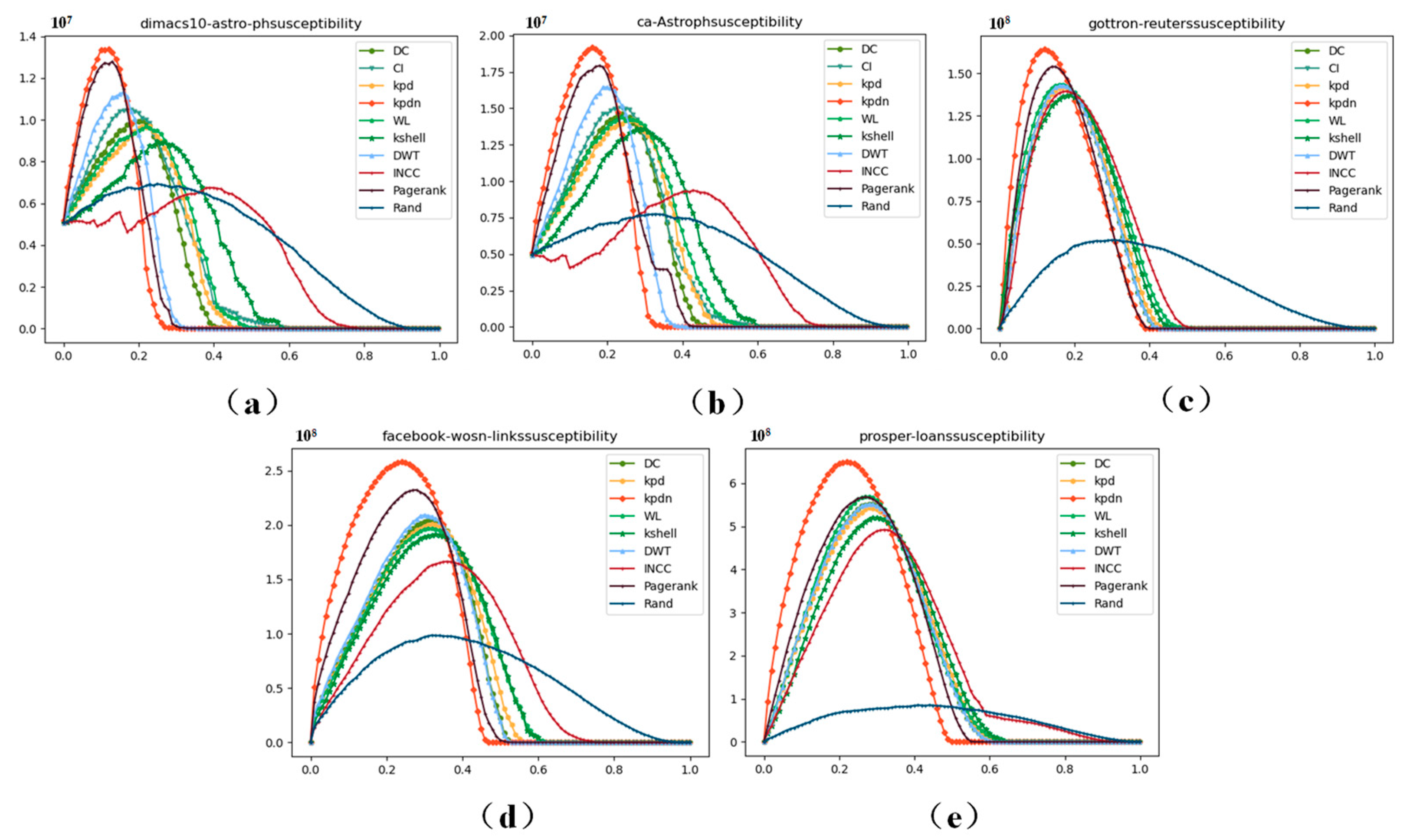
As can be clearly seen from Figure 9, on the newly added network data of scale ${10}^4\sim {10}^5$, the KPDN method can achieve suitable results in terms of subgraph sensitivity, meaning the proposed method has relatively high efficiency in node removal on real-world networks of scale ${10}^4\sim {10}^5$. Meanwhile, to describe the actual node removal ratio when different methods reach the extreme points in more detail, we summarize the extreme points obtained by the five real-world datasets under different strategies in Table S3 of Supplementary File S3.

As shown in Table S3 of Supplementary File S3, across the five datasets of scale ${10}^4\sim {10}^5$, compared with other classic algorithms, the KPDN method can decompose the original network more rapidly by removing fewer nodes.

5.2. Analysis of Artificial Networks

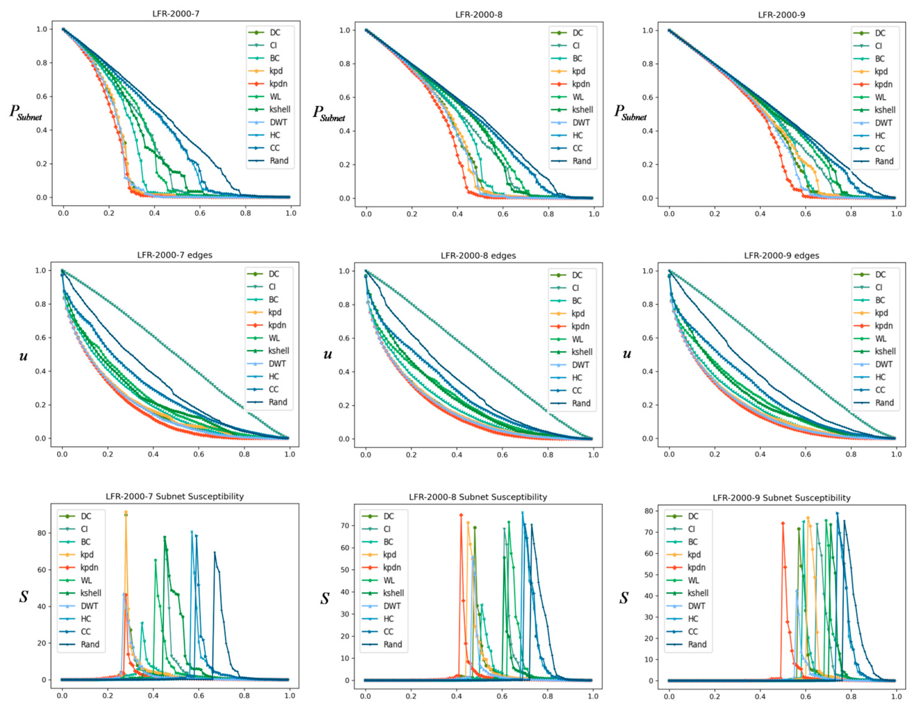
We also checked the performance of the proposed algorithm on synthetic networks with a clear community structure, as shown in Figure 10. The basic configuration obtained by the LFR algorithm is: $N=2000$, $t1=3$, $t2=1.5$, $mu=0.1$. In order to compare different average degrees, we set the average degree to 7, 8, and 9, respectively. Each column from left to right corresponds to the LFR networks with an average degree of 2.131, 3.448, and 4.7565, respectively. The first row compares the connected coefficient. The second row compares the remaining connected edges. The third row compares subnet sensitivity. From the figure, we can easily find that the dividing advantage of the method proposed in this paper on the LFR network is still quite obvious.

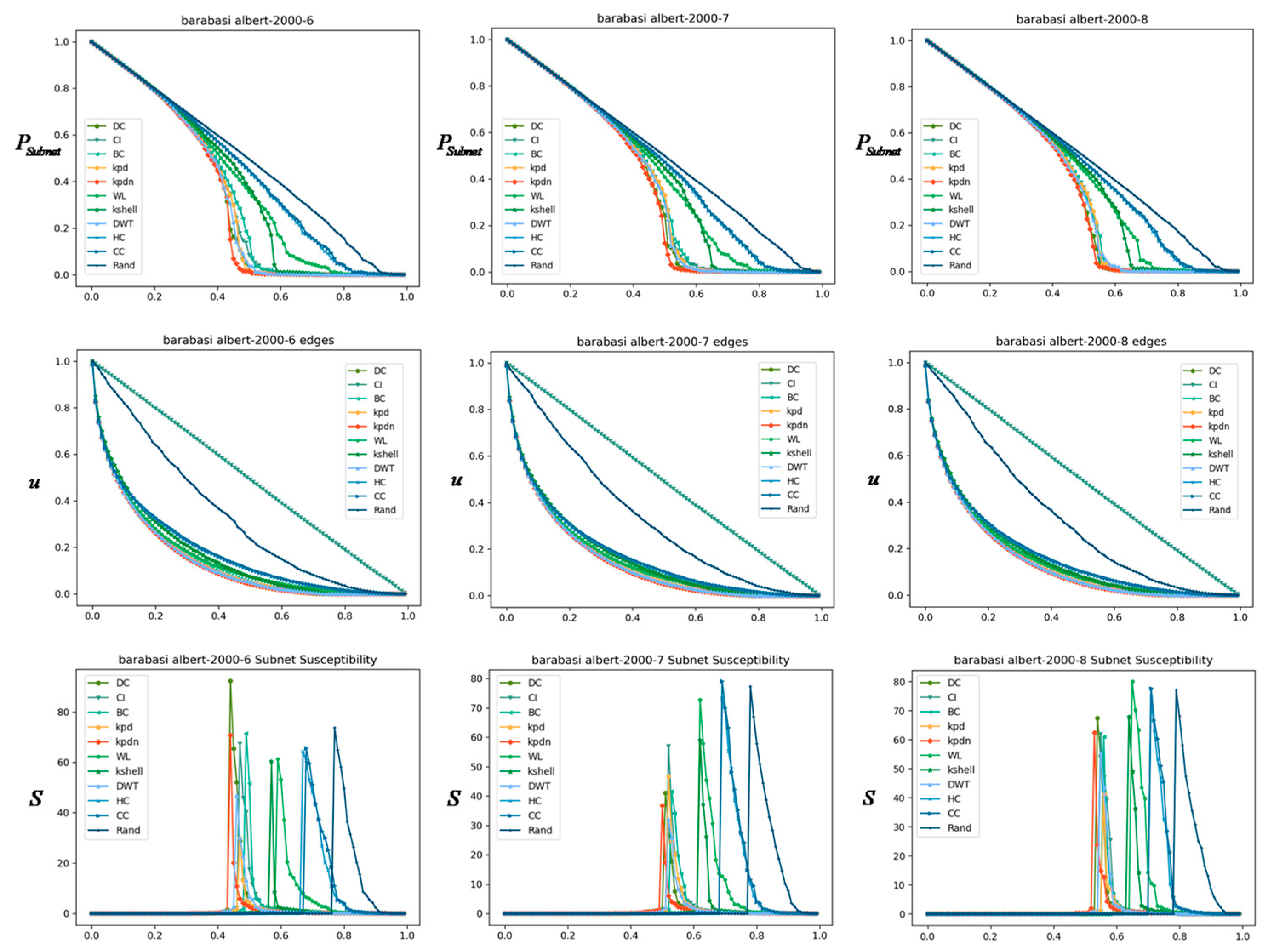
Similarly, we compared the small-world network, as shown in Figure 11. The basic configuration is: $N=2000$, $<k>$ = 3, 4 and 5, from left to right, the average degree is, as well as the Albert–Barabasi network, as shown in Figure 12. The basic configuration is: $N=2000$, $<k>$ = 6, 7, and 8, respectively.

Through the results shown in Figure 10, Figure 11 and Figure 12, the advantage of the KPDN method in analyzing important nodes in artificial networks is verified because the best performance is achieved in most cases and under different indicators. Especially for the LFR community networks and Watts–Strogatz small-world networks, we find that as the average degree of the network gradually increases, the effects of the subnet connectivity coefficient and sensitivity indicators are relatively more obvious. Compared with the Barabasi–Albert network, the effects of the three indicators of the proposed method are also in a leading or front position.

5.3. Result of Time and Space Complexity of Different Methods

We have organized the time complexity and space complexity of the various methods mentioned in this article. For detailed proof, please refer to Supplementary File S2. The results are shown in

Table 3. Time and space complexity of different methods.

Methods	Time Complexity	Space Complexity
DC	$O(n)$	$O(n)$
K-shell	$O(n+n\log n+e)$	$O(2n)$
CI	$O(n+\frac{e^2}{n})$	$O(n+\frac{e^2}{n})$
BC	$O(n^3)$	$O(n^3)$
WL	$O(e+n)$	$O(e+n)$
DWT	$O(n+e+\frac{e^2}{n})$	$O(n+2e)$
HC	$O(n^3)$	$O(n^3)$
CC	$O(n^3)$	$O(n^3)$
Pagerank	$O(2n+e)$	$O(2n+e)$
INCC	$O(n+\frac{e^2}{n}+2\frac{e^3}{n^2}+\frac{e^4}{n^3}+2e)$	$O(5n)$
KPD	$O(n+n\log n+e)$	$O(3n)$
KPDN	$O(2n+n\log n+e+\frac{e^2}{n})$	$O(4n+e)$

Note: Due to the inconsistency in the size of the number of nodes n and the number of edges e in different networks, we retain the number of nodes n and the number of edges e when calculating time and space complexity. According to the actual complexity network, subsequent researchers can calculate and compare by themselves with the size of $<k>$ (this paper considers the complexity of $<k>=\frac{e}{n}$ to be of the order of $O(1)$).

:

At the same time, it can be seen that although our time complexity and space complexity are not the smallest among all methods, they are not excessively large like methods such as BC, HC, CI, and CC. As we have stated, the complexity of the method proposed in this paper is not particularly high. Therefore, from the perspective of complexity analysis, the method proposed in this paper can be attempted on large-scale networks during actual use.

5.4. Result of Monotonicity of Different Methods

This paper measures the monotonicity of various algorithms. The higher the monotonicity of the algorithm, the stronger the ability of the method to determine a unique ranking. The bold text in

Table 4. Monotonicity results of real-world networks (scale ${10}^3–{10}^4$ ).

Methods	Email-Univ	US-Airports	Power-Eris1176	Bio-Grid-Worm	p2p-Gnutella08	Fb-Pages-Government
KPD	99.8463%	99.7662%	93.6236%	96.9196%	97.9375%	99.9788%
KPDN	99.9978%	99.8689%	97.8811%	97.9240%	99.9841%	99.9990%
DC	89.0558%	85.0127%	71.8568%	43.2396%	76.4186%	95.3086%
KSHELL	81.2117%	83.4311%	65.3067%	36.6958%	60.2274%	93.1956%
CC	99.9719%	99.8235%	98.7163%	97.8977%	99.9827%	99.9958%
DWT	98.8019%	99.8154%	94.8756%	94.7545%	92.7645%	99.3225%
CI	96.5451%	91.5538%	97.9252%	48.2129%	85.2549%	99.4984%
WL	99.8790%	99.8104%	94.1200%	96.9638%	97.7698%	99.9765%
HC	99.9981%	99.8761%	99.0951%	97.9289%	99.9876%	99.9990%
INCC	87.6090%	88.3489%	98.7560%	10.9898%	21.1736%	98.3378%
PR	99.9981%	99.9948%	98.9275%	97.9340%	99.9876%	99.9990%

and

Table 5. Monotonicity results of real-world networks (scale ${10}^4–{10}^5$ ).

Methods	Dimacs10-Astro-ph	Ca-Astroph	Gottron-Reuters	Prosper-Loans	Facebook-Wosn-Links
KPD	99.6912%	99.8508%	99.8725%	99.9987%	99.8928%
KPDN	99.8386%	99.9151%	99.9940%	99.9998%	99.9967%
DC	90.3604%	92.6562%	86.4161%	97.5723%	92.4147%
KSHELL	87.7731%	90.8483%	86.2097%	97.1114%	90.5103%
DWT	98.5433%	99.0495%	87.1266%	98.7977%	96.0803%
WL	99.6638%	99.8277%	99.9144%	99.9971%	99.8639%
INCC	98.2508%	98.8770%	68.5998%	79.2388%	90.3909%
PR	99.4724%	99.7526%	99.9989%	99.9998%	99.9971%

corresponds to the optimal value.

Although the monotonicity is not the best on some networks, the monotonicity of the KPDN method is higher than that of other algorithms on larger networks.

By comparing Table 4 and Table 5, we can see that for real-world networks of scale ${10}^3–{10}^4$, the monotonicity of our proposed method is second only to the PageRank method, but for networks of scale ${10}^4–{10}^5$, the monotonicity of both the KPDN method and PageRank rank high or first. Therefore, our proposed method also has some advantages in monotonicity for larger-scale networks.

6. Conclusions

This study aims to find a more general important node-sorting method suitable for complex networks with different characteristics. The proposed KPDN method comprehensively considers the global K-shell properties of nodes as well as the neighborhood properties of target nodes. Experiments show that the proposed method in this paper fully takes into account the local and global characteristics of nodes and performs well in identifying important nodes in most networks. At the same time, since the global characteristics are based on the K-shell method, there is no excessive time and computational burden in the overall consideration. Therefore, in general, the proposed method in this paper can better distinguish important nodes in most real-world networks. Meanwhile, it also has an obvious effect on identifying important nodes in similar community networks or networks satisfying the small-world property.

Moreover, this paper analyzes the importance of nodes from the perspective of network structure collapse. The work is mainly organized around the method of static node deletion in networks. Complex network models of real scenarios, such as virus propagation, have strong dynamic characteristics. According to the literature [32,33], the network structure status will change after each node deletion (for example, some indicators in Figure 2 and Figure 3 will show a curve with a slow decrease). Whether the changed network can inspire us to dynamically update the screening of nodes based on the initial node sorting method is worth further exploring. In recent years, the representation and analysis of multilayer networks and research on propagation dynamics based on complex networks have also been popular topics. These directions are also worth our in-depth exploration in the future.

References

1. Onnela, J.P.; Saramäki, J.; Hyvönen, J.; Szabó, G.; Lazer, D.; Kaski, K.; Kertész, J.; Barabási, A.L. Structure and tie strengths in mobile communication networks. Proc. Natl. Acad. Sci. USA 2007, 104, 18. [Google Scholar] [CrossRef] [PubMed]
2. Patacchini, E.; Zenou, Y. The strength of weak ties in crime. Eur. Econ. Rev. 2007, 52, 2. [Google Scholar] [CrossRef]
3. Li, G.; Hu, J.; Song, Y.; Yang, Y.; Li, H.-J. Analysis of the terrorist organization alliance network based on complex network theory. IEEE Access 2019, 7, 103854–103862. [Google Scholar] [CrossRef]
4. Pastor, S.R.; Vespignani, A. Immunization of complex networks. Phys. Rev. E Stat. Nonlinear Soft Matter Phys. 2002, 65, 036104. [Google Scholar] [CrossRef] [PubMed] [Green Version]
5. Liu, W.; Matteo, P.; Wu, A.P. Identification of Bridging Centrality in Complex Networks. IEEE Access 2019, 7, 93123–93130. [Google Scholar] [CrossRef]
6. Yu, E.Y.; Fu, Y.; Tang, Q. A reranking algorithm for identifying influential nodes in complex networks. IEEE Access 2020, 8, 211281–211290. [Google Scholar] [CrossRef]
7. Sebastian, W.; Sun, X.Q.; Massimiliano, Z.; Shlomo, H. QRE: Quick Robustness Estimation for large complex networks. Future Gener. Comput. Syst. 2018, 83, 413–424. [Google Scholar] [CrossRef]
8. Ryan, G.; Mahdi, J.; Yu, X.H. Correlation of cascade failures and centrality measures in complex networks. Future Gener. Comput. Syst. 2018, 83, 390–400. [Google Scholar] [CrossRef]
9. Bonacich, P. Factoring and weighting approaches to status scores and clique identification. J. Math. Sociol. 1972, 2, 113–120. [Google Scholar] [CrossRef]
10. Freeman, L.C. Centrality in social networks conceptual clarification. Soc. Netw. 1978, 1, 215–239. [Google Scholar] [CrossRef] [Green Version]
11. Massimo, M.; Vito, L. Harmony in the small-world. Phys. A Stat. Mech. Its Appl. 2000, 285, 539–546. [Google Scholar] [CrossRef] [Green Version]
12. Kitsak, M.; Gallos, L.K.; Havlin, S.; Liljeros, F.; Muchnik, L.; Stanley, H.E.; Makse, H.A. Identification of influential spreaders in complex networks. Nat. Phys. 2010, 6, 11. [Google Scholar] [CrossRef] [Green Version]
13. Estrada, E.; Rodríguez Velázquez, J.A. Subgraph centrality in complex networks. Phys. Rev. E Stat. Nonlinear Soft Matter Phys. 2005, 71, 056103. [Google Scholar] [CrossRef] [PubMed] [Green Version]
14. Morone, F.; Makse, H.A. Influence maximization in complex networks through optimal percolation. Nature 2015, 524, 7563. [Google Scholar] [CrossRef] [Green Version]
15. Morone, F.; Min, B.; Bo, L.; Mari, R.; Makse, H.A. Collective Influence Algorithm to find influencers via optimal percolation in massively large social media. Sci. Rep. 2016, 6, 1. [Google Scholar] [CrossRef] [Green Version]
16. Zeng, A.; Zhang, C.J. Ranking spreaders by decomposing complex networks. Phys. Lett. A 2013, 377, 14. [Google Scholar] [CrossRef] [Green Version]
17. Wang, M.; Li, W.C.; Guo, Y.N.; Peng, X.Y.; Li, Y.X. Identifying influential spreaders in complex networks based on improved k-shell method. Phys. A Stat. Mech. Its Appl. 2020, 554, 124229. [Google Scholar] [CrossRef]
18. Bae, J.Y.; Kim, S.W. Identifying and ranking influential spreaders in complex networks by neighborhood coreness. Phys. A Stat. Mech. Its Appl. 2014, 395, 549–559. [Google Scholar] [CrossRef]
19. Li, D.; Xi, J.K.; Sun, C.C. Node importance ranking algorithm with fusing degree and K-shell iteration number. Comput. Eng. Des. 2019, 40, 1518–1522. [Google Scholar] [CrossRef]
20. Xiong, C.Q.; Gu, X.H.; Wu, X.Y. Evaluation method of node importance in complex networks based on K-shell position and neighborhood within two steps. Appl. Res. Comput. 2022, 40. [Google Scholar] [CrossRef]
21. Xie, L.X.; Sun, H.H.; Yang, H.Y.; Zhang, L. Key node recognition in complex networks based on the K-shell method. J. Tsinghua Univ. (Sci. Technol.) 2022, 62, 849–861. [Google Scholar] [CrossRef]
22. Wang, J.W.; Rong, L.L.; Guo, T.Z. A new measure method of network node importance based on local characteristics. J. Dalian Univ. Technol. 2010, 50, 822–826. [Google Scholar]
23. Ruan, Y.R.; Tang, J.; Hu, Y.L.; Wang, H.R.; Bai, L. Efficient Algorithm for the Identification of Node Significance in Complex Network. IEEE Access 2020, 8, 2972107. [Google Scholar] [CrossRef]
24. Cheng, W.; Yang, B.; Zhang, R.; Wu, Q.; Zhu, B.; Liu, Z.; Xi, H.; Niu, K. Research on Key Node Identification Method of Transmission Network based on Improved PageRank Algorithm. In Proceedings of the 41st Chinese Control Conference (CCC2022), Hefei, China, 25–27 July 2022; pp. 5056–5061. [Google Scholar]
25. Dayong, Z.; Yang, W.; Zhaoxin, Z. Identifying and quantifying potential superspreaders in social networks. Sci. Rep. 2019, 9, 14811. [Google Scholar]
26. Ahmad, R.A.; Justin, M.; Mahdi, J.; Hamid, K. A machine learning-based approach for vital node identification in complex networks. Expert Syst. Appl. 2023, 214, 119086. [Google Scholar]
27. Lü, L.Y.; Chen, D.B.; Ren, X.L.; Zhang, Q.M.; Zhang, Y.C.; Zhou, T. Vital nodes identification in complex networks. Phys. Rep. 2016, 650, 1–63. [Google Scholar] [CrossRef]
28. Martin, D. Introduction to modern information retrieval. In Information Processing & Management; Salton, G., McGill, M., Eds.; McGraw-Hill: New York, NY, USA, 1983; Volume 19. [Google Scholar] [CrossRef]
29. Watts, D.J.; Strogatz, S.H. Collective dynamics of ‘small-world’ networks. Nature 1998, 393, 6684. [Google Scholar] [CrossRef]
30. Lancichinetti, A.; Fortunato, S.; Radicchi, F. Benchmark graphs for testing community detection algorithms. Phys. Rev. E Stat. Nonlinear Soft Matter Phys. 2008, 78, 046110. [Google Scholar] [CrossRef] [Green Version]
31. Stauffer, D.; Meyer, O.H. Simulation of consensus model of deftuant et al. on a Barabasi-Albert network. Int. J. Mod. Phys. C Phys. Comput. 2004, 15, 2. [Google Scholar]
32. Liu, Y.Y. Attack vulnerability of complex networks with different initial failure. In Proceedings of the 35th Chinese Control Conference (CCC2016), Chengdu, China, 27–29 July 2016; pp. 1293–1296. [Google Scholar]
33. Marialisa, S.; Aurelio, C.L. A Complex Insight for Quality of Service Based on Spreading Dynamics and Multilayer Networks in a 6G Scenario. Mathematics 2023, 11, 423. [Google Scholar]
Figure 1. Flow chart of the KPD method and KPDN method (as shown in the figure, the white box indicates the flow chart of the KPD method, and the gray box indicates the flow chart of the KPDN method).
Applsci 13 08303 g001
Figure 2. Comparison of the KPD method (df) and K-shell method principle (ac).
Applsci 13 08303 g002
Figure 3. Comparison of node deletion in a small-world network.
Applsci 13 08303 g003
Figure 4. Robustness comparison of 10 methods for node removal in real networks (results of maximum connected coefficient. The horizontal axis represents the proportion of nodes removed, and the vertical axis represents the subnetwork maximum connectivity coefficient). (af) correspond to: (a) email-univ, (b) p2p-Gnutella08, (c) fb-pages-government, (d) US-airports, (e) power-eris1176, and (f) bio-grid-worm.
Applsci 13 08303 g004
Figure 5. Comparison of subgraph sensitivity on real-world networks (scale 103–104). (af) correspond to: (a) email-univ, (b) p2p-Gnutella08, (c) fb-pages-government, (d) US-airports, (e) power-eris1176, and (f) bio-grid-worm.
Applsci 13 08303 g005
Figure 6. The decrease rate of network edges affected by different network disintegration strategies (proportion of remaining subnet edges. The horizontal axis represents the proportion of nodes removed, and the vertical axis represents the remaining ratio of edges in the subnetwork). (af) correspond to: (a) email-univ, (b) p2p-Gnutella08, (c) fb-pages-government, (d) US-airports, (e) power-eris1176, and (f) bio-grid-worm.
Applsci 13 08303 g006
Figure 7. The size of the largest connected component of the 5 newly added datasets of scale 10 4 10 5 . (ae) correspond to the datasets of: (a) dimas10-astro-ph, (b) ca-Astroph, (c) gottron-reuters, (d) facebook-wosn-links, and (e) prosper-loans.
Applsci 13 08303 g007
Figure 8. The maximum number of remaining edges of the 5 newly added datasets of scale 10 4 10 5 . (ae) correspond to the datasets of: (a) dimas10-astro-ph, (b) ca-Astroph, (c) gottron-reuters, (d) facebook-wosn-links, and (e) prosper-loans.
Applsci 13 08303 g008
Figure 9. Sensitivity values of the 5 newly added datasets of scale 10 4 10 5 . The data in (ae) correspond to: (a) dimas10-astro-ph, (b) ca-Astroph, (c) gottron-reuters, (d) facebook-wosn-links, and (e) prosper-loans.
Applsci 13 08303 g009
Figure 10. Comparison of LFR community networks, where each row from left to right has an average degree of 2.131, 3.448, and 4.7565, respectively. The first row compares the connected coefficient. The second row compares the remaining connected edges. The third row compares the subnet sensitivity.
Applsci 13 08303 g010
Figure 11. Comparison of small-world networks (average degrees are 3, 4, and 5 from left to right).
Applsci 13 08303 g011
Figure 12. Comparison of Albert–Barabasi networks (average degrees are 6, 7, and 8 from left to right).
Applsci 13 08303 g012