Multilayered Emergent Phenomena Caused by Basic Income and Labor Supply on the Wider Economic System

Abstract

Despite the growing interest in basic income (BI) in recent years, the existing research has mainly focused on its impact on household finances. However, changes in household behavior may affect the actions of other decision makers, such as businesses and governments, leading to unanticipated outcomes. Therefore, any analysis of BI must use a model with multilayered feedback from the actions of individual decision makers. To actualize such a model, household budgets, firms, and other entities must autonomously determine production levels, prices, and other factors, thereby encompassing a complete circulation of funds. This study constructs a macroeconomic model using agent-based modeling as a basic framework to achieve these goals, and it analyzes the emergent behaviors generated by BI and the labor supply in the economic system. The results show that although BI brings about more equitable consumption by households, it also creates a unique phenomenon wherein Gross Domestic Product increases but economic activity in terms of capital investment stagnates. Upon examining the impact of BI, the results of this study present the need to examine the multilayered feedback influencing mutual decision makers, which arises from the behavioral changes of individual decision makers caused by BI.

1. Introduction

Basic income (BI) has gained considerable attention as a new method of delivering social welfare [1,2], and empirical experiments and result analyses [3,4] have been conducted on the subject. However, there are some negative views of BI. Standing summarizes thirteen representative negative opinions [2], the most common being the problem of reduced labor supply. In this view, it is assumed that providing money may cause idle people to stop working.

There is much debate among proponents and detractors regarding BI and the willingness to work. Looking at the trends in this research, the studies that have analyzed previous demonstration experiments involving negative income taxes and subsequent fieldwork tended to generate more positive opinions. In contrast, the studies examining BI from the economic theory perspective tended to generate negative opinions. Although both approaches offer new insights, they also have problematic areas.

Regarding the analyses of the demonstration experiments, it is possible that changes made at the planning stage may have altered the effectiveness of individual BI systems [5,6] and caused phenomena such as the Hawthorne effect [7], with many questions about the social effects of large-scale implementation remaining unresolved [8].

At the same time, some argue that few theoretical approaches have been taken in the analyses based on economic theory [9], and there are examples where both negative and positive results have been derived [10]. For example, quantitative macroanalysis [11] and analysis using microsimulation [12] have produced conflicting results, such as a decrease in labor supply in one and no impact on labor supply in another [13]. Furthermore, the critique of BI in theoretical studies has been criticized by proponents as “one-handed economics” [2] that does not consider the feedback effects of BI.

Summarizing the issues with both approaches, the research conducted on demonstration experiments cannot conclusively clarify the facts of full-scale implementation due to limitations in the subject scope and time constraints. Moreover, the theoretical studies have been unable to consider feedback from the effects of BI implementation. In particular, the theoretical approaches cannot encapsulate individual judgments and decisions about work motivation-related reactions in their models.

An approach that would compensate for both of these problems is needed to conduct a full BI impact analysis because BI is an exogenous macroeconomic phenomenon that involves a massive change in the distribution channels of funds. Another reason is that the macrophenomenon involves changes in individual work incentives and feedback from interactions with surrounding stakeholders, as observed in demonstration experiments. Furthermore, regarding these interactions, there is a chance of double or triple feedback occurring where changes in household budgets affect firms’ production and investment, which can in turn influence household budgets.

Therefore, any impact analysis of BI requires a modeling approach that (1) can mimic the impact on the overall social system to the greatest extent possible; (2) can analyze the economic feedback that occurs when BI is implemented over time; and (3) can allow for a behavioral economic setting for individual household budget decision making. Agent-based modeling (ABM) provides an effective approach to this type of modeling. This study aims to construct an agent-based computational economics (ACE) model with a fully functional circulation of funds between households and firms that can be used to analyze emergent macroeconomic phenomena. It then seeks to use this model to analyze the impact of changes in labor supply caused by the effects of the implementation of BI on the economic system.

The simulation results show that by assuming some reduction in the willingness to work and a common change function for work motivation, BI would increase society’s overall well-being with more households consuming more goods. However, higher levels of BI benefits would adversely affect competitive economic activities, such as investment and production.

This paper contributes by demonstrating a newly emergent phenomenon that can be analyzed using a model encompassing detailed individual decision making, such as changes in work motivation, and the multilayered feedback of that behavior into the economic system when analyzing the impact of BI. Furthermore, we constructed an ACE model that includes a full circulation of funds between households and firms and a self-regulating function for capital investment and output to achieve these goals. The model presents complex emergent examples of the economic effects of changes in labor motivation resulting from implementing BI.

This paper is organized as follows. Section 2 summarizes the prior research and ABM. Section 3 provides an overview of the ACE model used in this study. Section 4 describes the conditions assumed in this study and the experimental parameters. Subsequently, Section 5 presents the experimental results, Section 6 discusses the results, and Section 7 presents the conclusions.

2. Prior Research and the Positioning of This Study

Basic income (BI) is a social policy that has received widespread public attention in recent years as an alternative to various social welfare programs. BI has been hailed as a kind of ideal social policy because it reduces the operational costs of social welfare, which entail enormous expenses [14], and frees people from forced subordination to poverty-based labor [1,15]. There also exist older ideas similar to BI, such as the proposals by Agrarian Justice [16] and others. In the 1970s, a negative income tax was first suggested [17], and many demonstration experiments were conducted in the United States [7,8]. A negative income tax has social implications and ethics and norms which are different to those of BI [18]. However, these empirical experiments have similar characteristics, and their results are also used in the considerations related to BI [7]. Gibson [8] synthesized the analytical studies of these empirical experiments, including the impact on health [14,19,20], the labor market [7,15,21,22], the educational effects, and family relationships. Rather than negative income taxes, BI experiments have been conducted in Finland [3] and California [4] in recent years in response to the growing BI debate, and the results have been subjected to analysis [23]. Based on these results, some have argued that it is already satisfactory as a proof of concept [24].

Some people question the system’s effectiveness [25], and some believe unemployment insurance is more beneficial than BI [26]. In addition to the aforementioned labor supply issues, there is the financial side; Hoynes states that implementing BI in the U.S. would require an amount equivalent to about 75% of total federal government spending in 2017 [25]. However, the issue that has drawn the most attention from BI’s opponents is labor supply. Several counterarguments have been presented that argue that although a slight reduction in work motivation may be observed, it is not a major issue. This is evidenced by experiments such as the negative income tax demonstration mentioned earlier [7,15,23,27,28,29].

However, some have argued that the demonstrations are problematic because of the way the experiments are set up and because of the changes in the implementation planning phase [5,6]. Moreover, a Hawthorne effect-like phenomenon may have occurred during the demonstrations [7]. If BI were implemented uniformly for all citizens, the response would be different. Furthermore, since the demonstrations used time-limited BI, it is conceivable that the behavior of the participants may be different from that in a situation in which permanent payments were guaranteed (e.g., behavior that views the period of payments as a period of preparation until after the payments are completed) [9,21]. Even in the positive camp’s theoretical framework, a temporary decrease in the labor force is still assumed [25], and empirical experiments have observed a 5–13% decrease in the labor supply [8,21,30]. Although these studies have focused on households’ willingness to work, a similar analysis of the impact of BI on the labor market from a corporate perspective also found an 11% decrease in labor supply [31], suggesting that a labor force decrease of around 10% would likely occur.

As such, the analysis of BI and its relationship to the labor supply is still unclear. Forget’s work on the issue of BI presents an important and thought-provoking perspective on this labor supply issue. According to Forget, “The more of his friends who attend, the more likely he will attend” [32]. This perspective also includes the consideration of the possibility that work motivation may change depending on comparisons with the incomes of others. Although Clark has considered the potential impact of relative income equality on changes in work motivation [33], we are unaware of instances of such changes being modeled in the impact analyses of BI.

The relationship between BI and labor supply is a complex interactive event in which human psychology and behavior are influenced by the surrounding environment. Experimental economies are effective methods for the creation of events in which to explore actual human psychological trends, while computer simulations that reproduce human society are effective for the analysis of large-scale social effects.

Experiments have been attempted in experimental economies on the impact of distributional systems on labor supply [34], on the impact of the willingness to work based on gift exchange games [35], and on risky investment behavior [9]. These studies have indicated that BI does not decrease work motivation or reduce risk behavior. However, Haigner’s experiment [34] decreases universal BI as a final labor outcome.

Other studies using ABM have been conducted besides the aforementioned microsimulations [11,12,13]. ABM is a modeling approach in which an autonomous decision-making entity (agent) acts according to its own internal conditions. This allows the analysis of emergent phenomena resulting from interactions with other entities and the surrounding environment. ABM is a research method that can analyze economic behavior in laboratory experiments [36], handle a wider range of nonlinear movements than conventional models that rely on equilibrium assumptions [37], bridge the micro–macro gap [38], and serve as a new tool for modeling and empirical analysis [39]. Therefore, the strengths of ABM lie in the modeling of detailed individual micro-decision making that leads to the creation of macrophenomena through feedback, as with innovation diffusion [40,41,42,43]. In particular, economic matters have been focused on since the 2007 financial crisis [44], and ABM is now being used as an alternative to the dynamic stochastic general equilibrium model [45,46,47]; the latter was the primary analytical tool of mainstream economics, but it has not proven to be sufficiently robust. These characteristics make ABM an effective tool for analyzing the impact of BI [27].

There have been comparisons between unemployment compensation and BI using agent-based modeling (ABM) [26], the analysis of degrowth societies considering asymmetric actors [48], the impact analysis of BI on food access from the poor to the wealthy [49], studies comparing poverty benefits, and studies comparing BI with childcare assistance and other programs [50].

While most of the researchers have taken a positive view of the impact of BI, Fabre concluded that unemployment insurance is a better policy option because BI results in more people quitting the labor force, and Heikkinen called for BI to help with the need to reduce the labor supply for the purpose of degrowth.

These experiments have either focused only on the outcomes and their aggregation for the target households alone or, even when they take a macro perspective, only on the employment situation and costs over a short period of time. BI represents not only a major change in finances and a major impact on individual decision making but also a change that has a significant mutual impact from micro to macro because the emergence of these decisions affects society as a whole and feeds back to the individual and into finance. Considering BI from this perspective, both the negative and the positive opinions show different dimensions.

If, as BI’s detractors argue, a decline in work motivation reduces the labor force, this could reduce the productive capacity of society as a whole and lower the supply of goods. This decline in the productive capacity of society as a whole could worsen economic conditions, reduce tax revenues, and make it impossible to continue BI. However, firms may take measures to address the decline in work motivation, such as automating production and increasing incentives through higher salaries. In addition, the shortage of goods may lead to higher goods prices, and households may be required to work to make ends meet with a reduced motivation to work. The complex overlap in the timing of the actions of these individual decision makers can lead to phenomena that can greatly destabilize the economy.

Based on the opinions of BI’s proponents and the actual empirical results, there will be at least a temporary decline in output throughout the economy because of the release of workers from involuntary labor or because of the behavior of people looking for better conditions for work. In this case, too, firms may take voluntary measures, as described above, which may result in complex or unstable social declines as a result of interactions with households that eventually find a less involuntary place to work.

However, to the best of our knowledge, no BI research to date has focused on the interaction that occurs as a result of individual decision makers’ responses to the decline in productivity of society as a whole and to the decline in productivity that occurs as a result of BI implementation. Accordingly, this study uses ABM to build a model that can analyze the impact of multilayered feedback from BI. The model was also used to analyze the emergent phenomena of the impact of the implementation of BI on labor supply, which is one of the most attention-drawing issues in the studies of BI.

3. Model Overview

3.1. Overview of the ACE Model

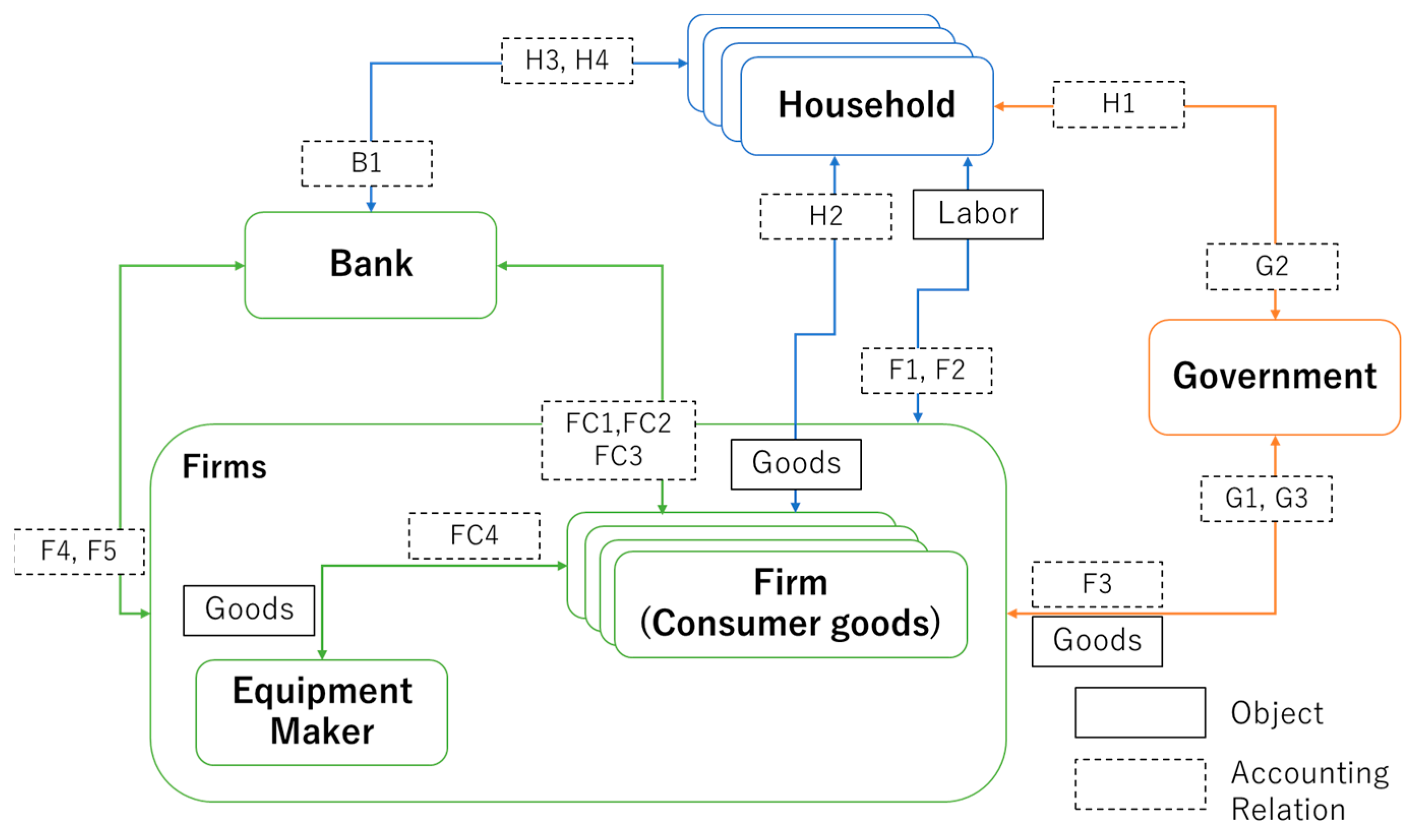
The model comprises five types of agents: households, which are the agents of labor and consumption; firms, which are the producers of employment and consumption goods; banks, which perform the money circulation function of the market; equipment makers, which are the producers of capital goods; and the government. It also makes the following assumptions with regard to the model as a whole.

• Types and preferences of consumer goods

  -

  There are I types of consumer goods to ensure market diversity.

  -

  Each firm produces two types of goods, which are randomly assigned at the beginning of the simulation from among the I types, but does not change its production type until the end of the simulation.

  -

  A competitive situation occurs in the market because multiple firms produce the same type of goods.

  -

  The production volume and prices of each product (type of goods) are adjusted by individual firms based on their own product sales.

  -

  Each consumer is assigned three market-recognizable types of consumer goods randomly at the beginning, and the types do not change until the end of the study.

  -

  The consumers’ preferences for each of the consumer goods are randomly assigned at the start.

  -

  The production equipment manufactured by the equipment makers shall always have a certain function (see production formula below) at a certain price, regardless of the product type or the state of the firm.

• Flow of funds within the market

  -

  Household income is determined by wages from firms, government subsidies, and interest from banks.

  -

  Firms’ funds are determined by sales to households, government subsidies, and borrowing from banks.

  -

  Government funding is determined by taxes paid by households and firms.

  -

  Funds in the system increase through bank credit creation, but not otherwise.

• Accounting-related tables and model overview charts

Table 1. Accounting-related tables.

ID	Sender’s Journal Entry						Accounting Relation	Receiver’s Journal Entry
	Sender	Type (Debit)	Subject (Debit)	Abstract	Subject (Credit)	Type (Credit)		Type (Debit)	Subject (Debit)	Abstract	Subject (Credit)	Type (Credit)	Receiver
H1	Hou	Liabilities	Accrued Income Tax	Accrued Income Tax Payment	Cash	Assets	Income Tax Payments	Assets	Cash	Income Tax Received	Income Tax Received	Revenue	Gov
H2	Hou	Expenses	Supplies_R	Buying Supplies_R	Cash	Assets	Buying CtoR Supplies (O)	Expenses	Cost of Sales	Product Sales C_Supplies	Products	Assets	FirCo
								Assets	Cash	Product Sales C_Supplies	Product Sales C_Supplies	Revenue
H3	Hou	Assets	Deposits	Deposits	Cash	Assets	Deposits	Assets	Cash	Deposits Under Custody	Deposits Under Custody	Liabilities	Ban
H4	Hou	Assets	Cash	Deposit Withdrawal	Deposits	Assets	Deposit Withdrawal	Liabilities	Deposits Under Custody	Deposit Withdrawal	Cash	Assets	Ban
F1	Fir	Liabilities	Accrued Fixed Salaries	Fixed Salary Payment	Cash	Assets	Fixed Salary Payment	Assets	Cash	Fixed Salary Received	Fixed Salaries Received	Revenue	Hou
F2	Fir	Liabilities	Accrued Bonuses	Bonus Payment	Cash	Assets	Bonus Payment	Assets	Cash	Bonus Received	Bonuses Received	Revenue	Hou
F3	Fir	Liabilities	Accrued Corporations Tax	Accrued Corporation Tax Payments	Cash	Assets	Corporations Tax Payment	Assets	Cash	Corporations Tax Received	Corporations Tax Received	Revenue	Gov
F4	Fir	Assets	Cash	Short-term Loans	Short-term Loans	Liabilities	Short-term Loans	Assets	Short-term Loan Receivables	Short-term Cash Loans	Cash	Assets	Ban
F5	Fir	Liabilities	Short-term Loans	Short-term Loan Repayments	Cash	Assets	Short-term Loan Repayments	Assets	Cash	Receive Short-term Repayments	Short-term Loan Receivables	Assets	Ban
FC1	FirCo	Assets	Cash	Long-term Loans	Long-term Loans	Liabilities	Long-term Loans	Assets	Long-term Loan Receivables	Long-term Cash Loans	Cash	Assets	Ban
FC2	FirCo	Liabilities	Accrued Interest (Facilities and Equipment)	Interest Payment	Cash	Assets	Interest Payment	Assets	Cash	Loan Interest Received	Interest Received	Revenue	Ban
FC3	FirCo	Liabilities	Long-term Loans	Long-term Loan Repayments	Cash	Assets	Long-term Loan Repayments	Assets	Cash	Receive Long-term Repayments	Long-term Loan Receivables	Assets	Ban
FC4	FirCo	Assets	Capital_E	Capital Buying_E	Cash	Assets	Buying RtoE Capital (O)	Expenses	Cost of Sales	Product Sales R_Capital	Products	Assets	FirEq
								Assets	Cash	Product Sales R_Capital	Product Sales R_Capital	Revenue
G1	Gov	Expenses	Corporate Subsidies	Corporate Subsidies Payment	Cash	Assets	Corporate Subsidies Payment	Assets	Cash	Subsidies Received	Subsidies Received	Revenue	FirCo
G2	Gov	Expenses	BI	BI Payment	Cash	Assets	BI Payment	Assets	Cash	BI Received	BI Received	Revenue	Hou
G3	Gov	Expenses	Supplies_R	Buying Supplies_R	Cash	Assets	Buying GtoR Supplies (O)	Expenses	Cost of Sales	Product Sales G_Supplies	Products	Assets	FirCo
								Assets	Cash	Product Sales G_Supplies	Product Sales G_Supplies	Revenue
B1	Ban	Expenses	Interest Expense (Interest)	Deposit Interest Payment	Cash	Assets	Deposit Interest Payment	Assets	Cash	Deposit Interest Received	Interest Received	Revenue	Hou
Hou: Household    Gov: Government    Ban:Bank    Fir: Firm & Equipment maker FirCo:    Firm (Consumer goods manufacturing)

presents the accounting-related tables [51] for the financial relationships among the agents in this model. The accounting-related tables indicate the financial transactions that occur between agents, with the left half of the table showing the journal entries for the agents that perform active actions and the right half indicating those of the agents that perform passive actions. The journal entries follow accounting rules. For instance, if cash, an asset item, appears on the journal side, it indicates that the transaction will increase the available cash. Figure 1 depicts the interrelationships of the agents in the model. The numbers written on the lines drawn between the agents in the figure are the numbers from the accounting-related tables. In addition, although Gross Domestic Product (GDP) and other data are compared in the simulation results of this model, GDP is calculated from these accounting data by calculating an input–output table for each period. Table 1 and Figure 1 are complementary representations of this model. Figure 1 is a conceptual representation showing that the funds in the model circulate among the agents and that the funds originating outside this loop do not flow into the model. This is shown specifically in the accounting-related tables in Table 1. All the monetary transactions between the agents included in this model are represented in the accounting-related tables. Therefore, this model shows that household income is paid out of corporate sales and that corporate sales are derived from the outlay of household income. Furthermore, the government collects and redistributes taxes from households and businesses, and the funds borrowed from banks for capital investment circulate in the market and are returned to the banks again, forming a complete capital circulation model.

• Order of actions

In this model, the actions are performed with the following steps, and the steps in this process are assumed to cycle within a time interval of one month in real time, which is also referred to as one period. The number listed for each step is the number from the accounting-related tables, and the corresponding numbered transactions in each step are made between the agents.

• Decision making and budgeting (H3, H4, F4)

Each agent determines its budget for tax payments and the amounts to be used for consumption, salaries, and grants according to the results of the previous fiscal year. Firms also make production plans and determine prices and production volumes according to the product sales in the previous period. In addition, the households determine their willingness to work in a given period based on their income status up to the previous period.

2.

Product manufacturing

Firms produce products based on the production plan made in 1. At this time, the amount of production may vary depending on the motivation of each worker (household) affiliated with the production process, and it may not be possible to meet the original demand.

3.

Consumables purchasing (H2, G3)

Households, as well as the government, make purchases according to their rules of purchasing behavior in line with their budgeted money.

4.

Tax payments (H1, F3)

Households and firms pay taxes according to the budgeted amount calculated in 1.

5.

Subsidies (G1, G2)

The government will provide subsidies to firms and BI to households according to its budget amount.

6.

Payroll (F1, F2)

Firms and equipment makers pay households a fixed salary, and a bonus is calculated from their profits at the end of the previous fiscal year. However, households are paid based on their willingness to work.

7.

Capital expenditure (FC1, FC4)

Firms make capital investments when they determine that demand is high based on the sales of their products.

8.

Debt repayment (F5, FC2, FC3)

Firms repay the bank with interest if they have borrowed money.

9.

Interest payments (B1)

Banks pay interest to households.

10.

Settlement of accounts

Each agent closes its books after one fiscal year and calculates profits, taxes, etc.

3.2. Agents

3.2.1. Households

Income and Consumption

The households are affiliated with firms or equipment makers and earn a wage, W, in exchange for providing labor. In addition, we assume that each individual receives basic income BI from the government and deposit interest DI from the bank, which, together with wages, constitute income Y (1). In addition, a portion of the wages is deducted in tax payments according to the income tax rate r_{i_tax}.

$${\mathrm{Y}}_{t-1}=W_{t-1}^h\left(1-r_{i\_tax}\right)+B{I}_{t-1}+D{I}_{t-1}^h$$

(1)

Using a Keynesian consumption function from Y, a portion is saved, and the remainder is used as budget C for consumption (2). In addition, deposits are randomly withdrawn and used for consumption, using the deposit withdrawal rate wd in each period to substitute for the purchases of capital goods and to prevent a bias of funds toward certain sectors.

$$C_t^h=bc+\left(Y_{t-1}^h-bc\right)mpc+D_t^{h}wd$$

(2)

Here, h denotes the index of households, t denotes the number of periods, bc denotes basic consumption, mpc denotes the marginal propensity to consume, and D denotes the amount of savings. Thus, $C_t^h$ denotes household h’s consumption budget in period t. The same rules apply to subsequent formulas.

Preferences

The households make purchases of consumer goods in the market based on C. The Cobb–Douglas type utility function is used for the purchase preferences. While there are I product types in the market, each household has n product types that it recognizes. The households then choose products to maximize utility U with C as the constraint (3).

$$U_t^h=u\left(x_1,\cdots ,x_i\right)={{\displaystyle \prod }}_{i=1}^n{x}_i^{{\alpha }_i^h}$$

(3)

$$\underset{\left(x_1,\cdots ,x_n\right)}{\max }{{\displaystyle \prod }}_{i=1}^n{x}_i^{{\alpha }_i^h}\cdots \mathrm{s}.\mathrm{t}. {{\displaystyle \sum }}_{i=1}^n{P}_i{}_t{x}_i\le C_t^h$$

Here, x_i denotes the amount of product i purchased, α is an elasticity parameter that sums to 1, and P_i is the price of product i.

Work Motivation

The households’ willingness to work varies with changes in income. In this study, for work motivation, we assume that it increases when one perceives one’s own income to be inferior to that of others [33]. In other words, we vary the work motivation M as shown in Equation (4), assuming that it decreases when one becomes richer than the others.

$$M_t^h=\frac{\delta }{\delta +e^{-\epsilon \left(\gamma \frac{Y_t^h}{Y_t^{ave}}-\gamma \right)}}$$

(4)

Here, γ, δ, and ε are parameters that allow us to determine the trends in work motivation as they change with respect to income. These parameters are explained in Section 3. In addition, Y_t^ave denotes the average income of all the households in period t.

3.2.2. Firms

Production Capacity

Firms adjust their output and prices each period according to the sales of the products they produce. As indicated in Equation (5), the production volume is determined by the Cobb–Douglas type function, where the upper limit $Q_{i_t}^{f\_lim}$ of the inventory that firm f can hold for product variety i is determined by its number of facilities K, the labor force L, and the coefficient a.

$$Q_{i_t}^{f\_lim}=a^f K_t^{f^{\beta }}{L}_t^{f^{1-\beta }}$$

(5)

In this case, K is the number of facilities owned and L is the labor force of employed workers. β is a parameter of the distribution ratio, with the assumption that the sum of the K and L exponents is 1. In addition, a is the value of technical skill given to each firm by a random number. Furthermore, L varies with the work ethic M_t^fh of the worker (household) fh belonging to firm f in the relevant period, as indicated in Equation (6).

$$L_t=\sum M_t^{fh}$$

(6)

Production Volume Determination

Firms determine the target production number $Q_{i_t}^{f\_lim}$ for each period using the periodic ordering method, with $Q_{i_t}^{f\_aim}$ as the actual upper production limit and the number of sales of the product up to the previous period. In this case, the forecast demand during the ti forecasting period is the average number of sales during the ti period. The safety stock is determined by the formula shown in Equation (7), assuming that the ordering interval is 1 and the procurement period is 0.

$$Q_{i_t}^{f_{aim}}=\frac{1}{ti}{{\displaystyle \sum }}_{j=t-ti}^{t-1}{Q}_{i_j}^{f_{sel}}+\left\{sa\sqrt{\frac{1}{ti}{{\displaystyle \sum }}_{j=t-ti}^{t-1}{\left(Q_{i_j}^{f_{sel}}-\frac{1}{ti}{{\displaystyle \sum }}_{ji=t-ti}^{t-1}{Q}_{i_j}^{f_{sel}}\right)}^2}\right\}-S{T}_{i_t}^f$$

(7)

Here, $Q_{i_j}^{f\_sel}$ is the sales volume of product i in period j, sa is the safety factor, and ST is the amount of inventory prior to production. As $Q_{i_t}^{f\_lim}$ is the upper production limit, the sum of $Q_{i_t}^{f\_aim}$ and ST will be $Q_{i_t}^{f\_aim}=Q_{i_t}^{f\_lim}-S{T}_{i_t}^f$ if it exceeds $Q_{i_t}^{f\_lim}$.

Pricing Determination

Prices are raised or lowered if the ratio of the previous period’s inventory to the production ceiling exceeds a threshold value. In this study, the price is raised by 2% when the inventory ratio is 20% and is lowered by 2% when it is 80%. However, the price is set so that it does not fall below the total cost of the product, which is calculated from the labor cost, depreciation cost, and interest on the borrowing incurred during the investment period.

Capital Investment

Capital investment is made to strengthen production capacity when inventory shortages persist for a certain period of time. Capital investment will increase K in Equation (5) to augment production capacity. The capital investment decisions are made by adding the investment flag variable in the period when $Q_{i_t}^{f\_aim}$ exceeds $Q_{i_t}^{f\_lim}$ in the production plan and subtracting the investment flag variable in the period when $Q_{i_t}^{f\_aim}$ falls below the current inventory of $S{T}_{i_t}^f$. In this paper, capital investment is made when the investment flag variable exceeds the investment decision threshold of 20. Half of the capital investment is financed by the firm’s own funds and half by long-term loans from banks.

Wages

The wage W^fh that a firm pays to each of its workers fh consists of a fixed salary W_f and a bonus. The amount of the fixed salary is randomly assigned to each household at the beginning of the simulation. However, the value of the fixed salary varies depending on work motivation. Bonuses are determined by the profit E^f_t derived from the previous period’s sales multiplied by the bonus rate r_b. However, this value is the total amount paid to the entire workforce, and the amount paid to individual workers varies with their work motivation for the period in question. Here, since the fixed salary can be considered to be each worker’s ability, worker fh’s share of the bonus is determined by the “fixed salary/total fixed salary paid to the employee” paid in period t. Thus, the amount each employee receives is as shown in Equation (8).

$$W_t^{fh}={\mathrm{W}}_f^{fh}{M}_t^{fh}+E_{t-1}^f{r}_b\left({\mathrm{W}}_f^{fh}{M}_{t-1}^{fh}/{{\displaystyle \sum }}_{fhi=1}^{fH}{\mathrm{W}}_f^{fhi}{M}_{t-1}^{fhi}\right)$$

(8)

The corporation’s tax rate r_{c_tax} is obtained from $E_t^f\left(r_b-1\right)$.

3.2.3. Government

The government collects taxes from households and firms and redistributes them. In this model, the government’s functions include government purchases (public spending), subsidies to firms, and a basic income for households.

In government purchasing, the government purchases consumable goods from the market in the same way as households do. In this study, for simplicity, the government purchases consumable goods as a substitute for government spending, including capital goods. The government sets purchasing resources from tax revenues according to a given government purchasing budget rate $g{r}_p$ and purchases market products equally for each producer and product number in turn for as long as the resources last. Firms are equally subsidized according to the firms’ subsidy budget rate $g{r}_s$. For simplicity, we assume that the firms receive the same subsidy amount regardless of their size.

Basic income distributes funds equally to households. The per capita grant amount $B{I}_t$ is the average of all the households’ incomes multiplied by the BI budget rate $g{r}_{BI}$ (9).

$$B{I}_t=g{r}_{BI}{Y}_{t-1}^{ave}$$

(9)

Notably, there are experimental conditions under which BI will not be implemented, but if BI is not implemented, the expenditures will be made according to the budgeted rates of the government purchases and firm subsidies described above. Furthermore, the conditions under which BI will be implemented will give priority to securing the necessary budget for BI, and the remaining amount will determine the budget for market purchases and subsidies according to the market rate.

3.2.4. Banks and Facilities

Banks have the effect of facilitating the flow of funds in the model. In the model, banks collect deposits from households and provide funds to firms for long-term loans when they make capital investments and for short-term loans when they have insufficient working capital. For long-term loans, interest is calculated based on the interest rate, and firms are required to repay the principal and interest in equal installments over a given repayment period. Long-term loans are assumed to be capped at a specified upper limit for multiple borrowings by the same firm over the same period. For simplicity, no interest is paid on short-term loans, as these loans are repaid in the following period. In this model, banks do not want to employ households, and charging interest would result in unlimited accumulation and stagnation of funds. Therefore, all interest payments are allocated according to the amount of household deposits for each period to prevent a bias of funds toward the banking sector.

Equipment makers produce equipment in response to orders from firms. As equipment makers also provide employment, they pay fixed wages and performance-based wages to affiliated households according to the sales obtained. In this study, the amount of equipment is fixed.

3.3. Basic Behavior of the Model

The basic behavior of the above model is described below. Figure 2 and Figure 3 indicate the results of the simulations without BI, with a = −0.02, m = 20, and γ = 50. The graph depicts the averages for each of the 12 periods in order to improve visibility.

As depicted in Figure 2, GDP and average product prices fluctuate up and down cyclically. Notably, the rise and fall of the average price lags behind GDP and is able to reproduce one of the stylized facts [52] that show that prices lag behind economic growth. In this model, production volume also rises and falls in response to demand, as indicated in Figure 3. It should be noted that the vertical axes of both Figure 2 and Figure 3 represent the monetary values as defined within the model. In the short term, firms use excess production capacity in tandem with price adjustments, and when firms determine that they still cannot meet demand, they respond by making capital investments. The production volume shows a gradual increase in the minimum. Meanwhile, the GDP and prices gradually decline with the repeated ups and downs. This happens because this model is a closed system, which means that the number of products in the market increases relative to the beginning of the simulation due to increased production capacity through capital investment; the model is a closed system and does not have population growth, trade, or other system expansions or transactions with external systems.

This business cycle is caused by the following sequence of events.

• Firms with a relatively strong competitive advantage in the market are unable to keep up with supply.
• Firms with competitive advantages borrow money from banks to make capital investments, which increases the amount of money flowing through the market.
• An increase in the quantity of funds improves household income and increases the demand for the products of the separate firms.
• Capital investment by separate firms creates a chain reaction of borrowing, increased capital circulation, and a cycle of capital investment.
• As capital expenditures run their course, the market is dominated by the repayment of funds rather than borrowing.
• As the funds begin to deplete the capital circulating in the market as the loans are repaid, a cycle occurs in which demand falls, prices fall, and wages fall.
• When the repayments reach their full maturity, a cycle of capital investment is generated again due to investment by the firms with competitive advantages.

In the economic models in which the above emergence occurs, there are changes in the work motivation, as indicated in Figure 4. The figure presents the percentage increase in GDP, cash, and deposits of all the households; the average of all the households’ work motivation, each averaged over one 12-period interval; and the percentage increase in the current period relative to the previous one. The cash and deposits of all the households increase and decrease in line with the growth rate of GDP. As for work motivation, we see that it is increasing and decreasing behind even these households. This is because as GDP rises, the feedback of the economic boom to households and the resulting disparities increase their work motivation, and as the economy slows, the motivation declines as income inequality shrinks.

4. Experiment Conditions

The purpose of this study is to observe the interaction and emergence of policies such as BI that have significant financial, material, and psychological effects in a system where labor motivation and market demand are fed back to output and prices and in which the full financial cycle is contained.

Looking at the parameters of the work motivation function in Equation (4) for the experimental conditions, the larger the value of γ and the closer the value of ε to 0, the slower the decrease in work motivation. The larger the value of δ, the more it shifts the starting position of the decrease in work motivation to the right. Figure 5 shows how work motivation in Equation (4) changes with the relative proportion of one’s income to the average income. The solid lines show the change in work motivation when the value of ε changes to −0.02, −0.06, and −0.1. Note that γ = 50 and δ = 20 are set as the additional parameters. The dashed lines in Equation (4) also show the extent to which the willingness to work changes when 50% of average income is provided as BI under ε = −0.02 and −0.01.

At ε = −0.02, one’s income is 100% of the average income and one’s willingness to work is about 5% less than when one’s income is 0. In addition, receiving a BI of 50% of average income in that condition would reduce work motivation by about 3%. This is an assumption that implies less reduction in work motivation than the results of previous studies [8,21], which demonstrated that a guaranteed minimum subsidy from a negative income tax would reduce work motivation by 5% to 10%. As a comparison condition, we also conducted the experiment with ε = −0.1, where the willingness to work decreased by 50% at 150% of average income.

Realistically, people with the ability and vitality to reach as much as 1000% of the average income may not decrease their work ethic as their income increases. Alternatively, it is possible that a small number of them possess a slothful work motivation function that would prevent them from working at all if they could earn nearly twice the average income. However, since this study focuses only on the emergence of BI on the above system, the experiment assumes that all households possess the same work motivation function.

The basic parameters of the simulation were performed under the conditions indicated in

Table 2. Basic parameters.

Simulation period T	360	Fixed wage Wf	4000~5000
Number of item type I	10	Basic consumption bc	1000~1500
Number of household H	500	Marginal propensity to consume mpc	0.5
Number of Firm F	60	Withdrawal rate wd (random every period)	0.5~0.8
Number of Government G	1	Update interval of working willingness	12
Number of Equipment maker E	1	Number of product type can be produced	2
Number of Bank B	1	Initial Equipment Kt	1
Initial Cash of household	3000~5000	a of Cobb-Douglas type production function	10~12
Initial Cash of firm	100,000	Capital distribution ratio β	0.2
Initial Cash of Government	100,000	Forecasted period ti	10
Initial Cash of Equipment maker	1,000,000	Safety coefficient sa	1.65
Initial Cash of Bank	40,000,000	Initial price of every firm’s goods	1000~1500
Budget rate for government purchases $g{r}_p$	0.5	Bonus ratio of firm rb	0.5
Budget rate for firm subsidies $g{r}_s$	0.5	Repayment period of long-term loan	100
Equipment price	500,000	Maximum number of long-term loans	2
Maximum production of equipment per period	10	Interest rate of loan	0.01

. Note that the basic behavior of the model shown in 2.3 was also performed under similar conditions and with ε = −0.02, r_{i_tax} = 0.2, and r_{c_tax} = 0.4. The experimental levels for analyzing the impact of BI are shown in

Table 3. Experiment levels.

	Condition I	Condition II
Parameters of labor motivation ε	−0.02	−0.1
Income tax rate ri_tax	0.2	0.2
Corporate tax rate rc_tax	0.4	0.4
BI budget rate grBI	No, 20%, 40%	No, 20%, 40%

. Condition I is a condition in which the decline in work motivation due to higher income is gradual, while Condition II is one in which the decline in work motivation is rapid. The simulations were conducted separately for the cases in which no BI was delivered; when BI was delivered for 20% of average income; and when BI was delivered for 40% of average income, respectively. The income tax rate r_{i_tax} and the corporate tax rate r_{c_tax} were set as values that would not be considered extreme following the findings of a previous study on the impact of government tax rates using the same family of models [53]. For gr_BI, we also referred to the hypothesis that the appropriate amount of BI is approximately 1/4 of GDP per capita [1,27]. As GDP per capita in OECD countries translates to 20–25% of annual income, the standard value for gr_BI was set at 20% and doubled to 40% as an experimental condition for comparison.

5. Results

Figure 6 presents the time series of GDP when there is no BI (NoBI) in Condition I and when BI is delivered at 20% (BI20%) and 40% (BI40%) of average income. Experimental levels of 60% and 80% were also tested, but no difference was observed above 40% because all of the collected tax revenues were used for BI.

Figure 6, which shows the time-series trend of GDP, shows that the bottom of the NoBI condition tends to be one level lower during economic downturns, but it is difficult to clearly distinguish the other trends. Therefore, a comparison using the average GDP over 360 periods, as shown in

Table 4. Effects of BI on GDP, output, prices, investment, and willingness under Conditions I and II.

	ε = −0.02			ε = −0.1
	NoBI	BI20%	BI40%	NoBI	BI20%	BI40%
GDP	4,020,115	4,457,200	4,423,324	3,900,102	4,486,099	4,547,055
Average production volume	4143	4056	3990	3937	3984	3821
Average price	904	1023	1036	932	1047	1106
Amount invested	14,634,086	14,069,123	13,119,279	13,654,263	14,013,064	13,792,490
Average work motivation	95.88%	95.68%	95.79%	95.23%	95.34%	93.85%
Minimum work motivation	88.90%	89.60%	88.50%	8.39%	20.68%	5.84%

, shows that GDP is higher in the conditions in which BI is delivered. Similarly, the amount of capital investment and the number of products and prices produced in the market, as shown in Table 4, indicate that the conditions without BI are more active than those with BI being granted. The comparison between BI20% and BI40% also shows that the benefits of BI tend to be more active with respect to investment and product production status, which is inversely proportional to the amount of BI benefits granted.

Furthermore, with respect to GDP, when ε = −0.02, BI20% resulted in a higher GDP than BI40%. This suggests that with regard to BI benefits, a higher benefit amount does not automatically translate into a healthier society. In fact, in the ε = −0.1 condition, i.e., a society with members who respond more rapidly to a decline in work motivation due to higher income, the BI20% condition outputs better results, with a higher GDP compared to NoBI and more investments being made than in the BI40% condition, as shown in Table 4.

Table 4 also displays the minimum work motivation of the agents who had the lowest work motivation during the simulation. At ε = −0.02, the minimum work motivation never falls below 80% because the decline in work motivation is gradual, even for very high earners. At ε = −0.1, the work ethic of high-income earners is set below 10% because the decline in work ethic accelerates rapidly from a certain point. However, the average work motivation for 500 and 360 periods is about 95% under both conditions.

Under the condition of ε = −0.1, BI20% GDP was slightly inferior to BI40%. However, capital investment was most active in BI20%. In conjunction with this, BI20% was also the highest in terms of production. Furthermore, with regard to minimum work motivation, the least decrease in work motivation occurred at BI20%. As for prices, the conditions without BI were the cheapest, but it is difficult to draw a general conclusion because prices are also affected by overall economic conditions. The optimal economic and social outcomes from these results for the impact of BI will be discussed in the next section.

6. Discussion

The results of the experiment show that GDP tends to be higher under BI benefit conditions than under NoBI conditions, while investment and other economic activities are also greater under NoBI conditions. One answer to the question of which is better is “the amount of product that households are able to consume”. Product output in this model is only determined by the firms’ decisions in response to market demand, and high output does not necessarily indicate that there are high numbers of households capable of consuming the goods. Even in societies with high GDP, many households are not well off due to lower consumption volumes, which are due to higher prices because of lower production. Therefore, Figure 7 presents the results of stratifying the number of products that households are able to consume from zero, one, and two to five, among others.

Figure 7 shows that under conditions with BI, there is a larger proportion of households that consume 6 to 10 products each period than under NoBI conditions. Furthermore, the product consumption layers of two to five are reduced in the conditions with BI compared to the conditions without BI. It was found that under NoBI conditions, the society was hyper-competitive and separated into a small segment of households that were able to consume large amounts (some households in the 21+ consumption segment consumed more than 70 units each quarter) and a larger segment of households that were able to consume only a small amount.

In addition, the group that consumed two to five units was the smallest at BI20% for those under ε = −0.1 conditions. Furthermore, BI20% produced a large variety of products while maintaining somewhat high prices; yet, an equal percentage of products was consumed, while GDP and investment thrived, making it the ideal situation of the three conditions.

These results indicate two implications: implementing BI tends to result in higher GDP, but investment is more active when BI is not implemented. This is the outcome of the impact of BI on both the financial cycle and the competitive aspects of the economic system in this model.

The main factor that increases GDP is the income redistribution effect of BI. In this model, in the absence of BI, a large portion of the tax revenue ultimately goes to firm sales as public spending. These sales become the savings of firms, the income of households, and the next source of government spending, and after several cycles, they are aggregated under firms with a competitive advantage, encouraging investment, and then further aggregated as profits to selected households. As a result, wealth is concentrated in the hands of a few firms and households, which impedes the flow of funds. As a result, the flow of funds deteriorates during economic downturns, lowering GDP. In contrast, BI, because it redistributes tax revenues evenly, has the effect of preventing wealth from being concentrated in the hands of a few firms and households and of giving even low-income individuals purchasing power, thereby preventing GDP deterioration during economic downturns.

The factors that lead to reduced investment as a result of BI are driven by reduced competition. Under the assumption that an increase in income decreases work motivation, the implementation of BI is likely to cause a decrease in work motivation. Therefore, firms with competitive advantages do not emerge, investment declines, and production tends to decrease. However, because of the distributional effects of BI, even low-income households can still purchase goods, and GDP tends to be comparatively higher under BI during economic downturns. These effects become more apparent the higher the amount of BI; so, both the work ethic and investment tend to be low under the 40%BI condition.

Because BI exhibits these two opposing effects, the results show that BI20% results in better social and economic outcomes than NoBI or BI40% under extreme conditions such as ε = −0.1. Even under the condition ε = −0.02, it is superior to NoBI in terms of GDP and superior to BI40% in terms of investment. Therefore, ε = −0.1 can be said to show the results of the extreme clarification of the respective effects.

From this, it can be inferred from the present results that the implementation of BI may, to a certain extent, bring about social well-being; however, an excessive level of BI weighting may not bring about positive results. Although this is not an elaborate model and is intended only as a reference, BI20% would be about 30% of the median income in real terms.

Although this is a middle-range model [54] and intended for reference purposes only, BI20% is approximately 30% of the median income in real terms. This figure is close to a quarter of GDP per capita, which is considered the appropriate level for BI [1,27]. As work motivation in this model is directly related to labor supply, the average decrease in work motivation due to an appropriate level of BI, ε = −0.02, is 5%. Even households with the largest decrease in work motivation over the 360 days modeled are only about 10%. This is not a significant departure from the 5–10% decrease in work motivation [7,8,30,31] observed in previous empirical studies. This suggests that our results mirror previous studies regarding the relation between BI and work motivation.

However, at the same time, the existing empirical studies have paid limited attention to the impact analyses of BI on the decision making of firms related to investment and production behaviors. These studies are limited to those that address the matter from a corporate perspective, noting that firms would be forced to raise wages due to decreased labor supply [31]. Conversely, macro-quantitative analyses [11] have taken multilayered feedback into account, leading to a decrease in capital due to a decrease in the amount of labor resulting from the implementation of BI. These studies have shown that implementing BI results in a decrease in GDP because BI leads to an increased decline in labor supply, and the decline in households’ self-preservation awareness contributes to reduced savings, resulting in a decline in overall capital and a deterioration in productivity. These findings differ from those of our model, which attempts to compensate for the decreased labor force through capital investment. A noteworthy difference in the results is that when considering the impact of the multilayered interactions caused by BI, individual firms will also experience differences due to factors that allow them to adapt autonomously to change.

7. Conclusions

This study focuses purely on the interaction effects of BI, which has significant financial, material, and psychological effects, and analyzes it using a system that incorporates a complete financial cycle in which labor motivation and market demand are fed back to production volume and prices.

The results show (1) that BI reduces work motivation to some extent and (2) that under the assumption that the changing function of work motivation is the same for all, the implementation of BI results in the creation of an equitable social environment in which a larger number of households are able to consume a greater amount of goods. Higher BI resulted in negative effects on competitive economic activities, such as investment and production. These results indicate that by incorporating a system of feedback in output and investment, BI has the dual nature of stimulating economic activity through income redistribution and of weakening economic activity through reduced competitiveness. Under the experimental conditions of this study, we found that a BI slightly lower than the amount that guarantees a minimum standard of living, as called for by the universal basic income, better serves social well-being and does more to enhance economic activity.

The results of this study show that providing a monetary figure close to the standard BI amount given in previous studies leads to a decreased labor supply, which aligns closely with the results achieved in empirical studies. However, the results suggest a unique economic outcome: an increase in GDP combined with a contraction in production, investment, and other business activities.

The above suggests that there may be an optimal point for BI implementation where social well-being and economic activity can be balanced and that it is important to consider using systems that incorporate feedback on capital investment and production volume.

Limitations of This Study and Questions for Possible Future Research

By analyzing the impact of BI using a model encompassing multilayered feedback, this study focused on emergent phenomena not previously considered by either the proponents or the opponents of BI. Therefore, the parameter settings used assumed values to confirm emergent phenomena. We also incorporated a hypothetical function of work motivation designed to decline when external income is earned. Therefore, for future research, it will be necessary to introduce more realistic work motivation functions and to incorporate research findings on relative wage disparities. As research on relative work motivation functions has been conducted by statistically analyzing survey data, future studies should use the results of these surveys to establish precise parameters.

Additionally, the current model does not incorporate the full scope of the labor market and does not address issues such as voluntary resignations, company layoffs, and job hunting. The labor market is a variable that interacts with work motivation and the expansion of production capacity through price and output adjustments and capital investment. Therefore, introducing a fully modeled labor market could lead to emergent effects that would further destabilize the economy due to the impact of BI. Therefore, further extending the model to analyze the impact of BI is something to consider in the future.

However, the results of this study reveal that analyzing the impact of BI from a macro, long-term perspective, with a multilayered feedback system structure and a macro, long-term perspective, results in the emergence of a unique phenomenon: an increase in GDP and a contraction in economic activity. Although this study focused on labor supply, this multilayered feedback could significantly impact overall market product volume, prices, and even technological progress. Thus, there is a concern that price fluctuations may cause the welfare, education, and health of people with low incomes to not improve with the introduction of BI, as anticipated by proponents. Furthermore, major economic system changes can significantly impact government finances and create further destabilizing behavior if the government adopts corrective policies. Therefore, based on the findings of this study, it can be argued that in examining the impact of BI, it is necessary to consider the multilayered feedback that each decision-making entity in society produces in response to change, such as the impact of BI on corporate activities.