Article

Commuted PD Controller for Nonlinear Systems: Glucose–Insulin Regulatory Case

by
Gisela Pujol-Vázquez
*,†,
Leonardo Acho
and
José Gibergans-Báguena
Department of Mathematics, Universitat Politècnica de Catalunya-BarcelonaTech (ESEIAAT), 08222 Terrassa, Spain
*
Author to whom correspondence should be addressed.
These authors contributed equally to this work.
Appl. Sci. 2023, 13(14), 8129; https://doi.org/10.3390/app13148129
Submission received: 14 June 2023 / Revised: 8 July 2023 / Accepted: 11 July 2023 / Published: 12 July 2023
(This article belongs to the Special Issue Research and Application of Intelligent Control Algorithm)

Abstract

:
As an option to deal with insulin-dependent disease, a recently commuted PD control strategy is designed and carefully analyzed for different clinic diabetic patients. This controller approach is mainly conceived to stabilize the glucose blood concentration in a diabetic patient around its basal value; hence, avoiding extreme situations such as hypoglycemia and hyperglycemia. This control strategy receives two inputs carefully tuned to actuate when the measured variable is out of a prescribed healthy zone. Therefore, one of these variables is invoked to decrease the glucose concentration to insulin injection, and the other is employed to increase the glucose absorption, both by using a proper PD controller. According to our numerical experiments, our controller approach performs well, even when there is an external disturbance in the controlled system.

1. Introduction

Diabetes (diabetes mellitus) is a chronic disease that affects millions of persons worldwide (see, for instance [1,2,3,4]). This disease is characterized by inadequate control of the blood glucose concentration in the body, leading to complications such as limb loss, blindness, ischemic heart disease, and end-stage renal disease [3]. Moreover, for diabetic patients with insulin-dependent diabetes, the glucose–insulin regulatory system can be viewed as a feedback-control example where the blood glucose levels are frequently measured to control it (see, for instance [2,5,6,7,8]). Additionally, according to the Diabetes Control and Complications Trial (DCCT), the blood glucose concentration should be within the range of 50–120 mg/dL [4]. In [9], the range from 60 mg/dL to 110 mg/dL is considered the normal blood glucose concentration level in humans. Therefore, by correctly applying insulin, this glucose level can be correctly (healthy) manipulated. For reference values, above 120 mg/dL, the state of the patient is known as hyperglycemia, and below 50 mg/dL, the state is known as hypoglycemia. Both states are harmful to diabetic patients [4]. Exogenous factors that can affect glucose include food intake, rate of digestion, exercise, and reproductive state, among others [2,4]. Hence, for control performance evaluation, it is also important that the designed controller be robust in front of any real kind of internal or external perturbations.
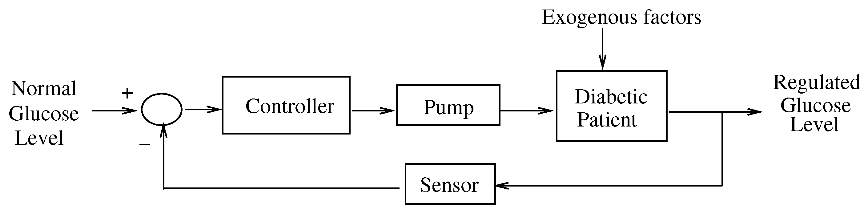
Figure 1 shows the block diagram of a closed-loop controlled system of diabetic patients using insulin pumps [4,6]. In this scheme, the glucose sensor can be embedded under the skin, and the insulin pump can be implanted in the abdomen. So, the control objective consists to keep regulating the glucose level in the body. In this scenario, the patient is said to be under metabolic control. The pump injects insulin through a catheter. The system shown in Figure 1 can be referred to as an artificial pancreas because this closed-loop system replaces, in some way, the pancreas activity in controlling the glucose level of the body of a healthy person [2].
In literature, several approaches have been used to design artificial pancreas. For instance, a robust controller using a higher-order sliding mode control was studied in [6]. Using optimal H control theory, an insulin injection control was analyzed in [5]. And employing a parametric programming approach for the control design was considered in [4]. On the other hand, in [10], control algorithms using standard linear control techniques, like the proportional-derivative controller, were studied, as in [11,12,13]. In this paper, the feedback measurement signal was assumed to be available at discrete-time moments which resulted in an interesting and useful technological fact for an artificial pancreas design. In contrast, we claim that no significant benefit is obtained from using a nonlinear model-based control design strategy. For instance, in [14], an impulsive model predictive control is presented, but the mathematical model has to be linear, and in [15], miss undertaken internal dynamics. On the other hand, PID controllers in the artificial pancreas have been studied in [16], but only for hyperglycemic conditions, and in [17] a PID robust control is presented for the hypoglycemic situation, but both conditions are not studied simultaneously, as in the present work. However, the nonlinear techniques can offer new ways of control implementation that can face some nonlinearities ignored in by the linear controller tools. Some of these nonlinear control design strategies involve sliding mode control [6,18], delay control [19], optimal control [20], switched LPV control [21], sub-optimal control [22], model predictive control [23], fuzzy control [24], reinforcement learning [25], etc. Therefore, the use of these control design tools allows us to innovate new developments for artificial pancreas approaches. Our proposal aims to act upon the control part of an insulin-dependent diabetic system to develop an effective and simple solution to avoid nondesired clinical problems.
The main objective of the present work is to design a robust control for an artificial pancreas to minimize the effect of extreme situations such as hyperglycemia or hypoglycemia. Additionally, we evaluate our artificial pancreas performance under different scenarios. Our control strategy uses a novel switched strategy: when a peak value on glucose blood concentration is detected, the controller tries to minimize its level by injecting insulin into the system, and when the glucose blood concentration is lower than a healthy level, glucose ingestion is administrated by the controller. The objective is to maintain a healthy level of glucose. The control strategy is based on a proportional-derivative (PD) theory, where the input signal is the detected peak value of the blood glucose concentration. The PD controller format is considered due to its simple and easy realization [11], as pointed out by [12,20]. We avoid using the PID controller because its integral action may be useless [13]. This is also evidenced, in our numerical experiments, noticing that strong hypoglycemia occurs during a long period of time when the integral part is considered. But, in order to complete the study of the proposed switched strategy, a reset integral part is considered, defining a commuted proportional integral derivative (PID) controller. This approach is based on Clegg integrator [26], where a reset signal is introduced to face the overshoots produced by the integral part of the controller as suggested in [27,28].
The rest of the paper is organized as follows. First, the nonlinear mathematical model and the proposed controller are presented in Section 2. Then, Section 3 shows the performance of the combined PD controller in different scenarios: with decaying disturbance; with external additive perturbation; and in the presence of dynamical plant changes. Also, in this section, a resetting PID is evaluated to see the undesired chattering effect due to the integral part of the control architecture. Finally, Section 4 discusses the obtained results, and conclusions are stated in Section 5.

2. Materials and Methods

2.1. Dynamical Model of the Glucose–Insulin Regulatory System

The main objective of this paper is to design a robust PD controller for an artificial pancreas able to stabilize the glycemia blood level around its basal value and prevent hypoglycemia from appearing when the administrated insulin is not well assimilated by the patient.
In the recent literature, there are some glucose–insulin regulatory mathematical models [29]. In this paper, we consider the minimal model called the Bergman minimal model [30], widely used in literature (see, for instance [4,5,6,10] and references therein). This is due to its simplicity. This model is as described follows:
x ˙ 1 ( t ) = p 1 ( x 1 ( t ) G b ) x 1 ( t ) · x 2 ( t ) + D ( t ) ,
x ˙ 2 ( t ) = p 2 x 2 ( t ) + p 3 ( x 3 ( t ) I b ) ,
x ˙ 3 ( t ) = n ( x 3 ( t ) I b ) + γ [ x 1 ( t ) σ ] + t + u ( t ) ,
where x 1 ( t ) , x 2 ( t ) and x 3 ( t ) are the blood plasma glucose concentration (mg/dL), the insulin’s effect on the net glucose disappearance (1/min) and the insulin concentration in plasma ( μ U/mL), respectively. [ x 1 σ ] + means that when x 1 ( t ) is greater that σ , the value is taken to be [ x 1 σ ] , otherwise, its value is zero. Bergman et al. [30] describe this factor as the feedback response of pancreatic insulin to variations in glucose concentration in the bloodstream. G b and I b are the basal value levels of pre-injection level of glucose (mg/dL) and the pre-injection level of insulin ( μ U/mL), respectively. These values can be also called the subject’s baseline glycemia ( G b ) and the subject’s baseline insulinemia ( I b ) [19]. Remark that σ is greater than G b . D ( t ) represents the exogenous factors, and u ( t ) defines the insulin injection rate being the control input. Parameters p 1 , p 2 , p 3 , n and γ are the system parameters. These are described, for instance, in [6,19]. Additionally, x 1 ( 0 ) , x 2 ( 0 ) , and x 3 ( 0 ) are the corresponding initial conditions. Finally, x 1 ( t ) is the available output system for the control algorithm.
The term D ( t ) represents the rate at which glucose enters to the bloodstream from intestinal absorption after food intake. In oral glucose tests with nondiabetic subjects, the model aims to produce the desired effect that the plasma glucose level rises too rapidly (from the resting level) to a maximum in less than 30 min and then falling to the base level after 2–3 h [20]. Moreover, the exponential function also produces the desired behavior for the model.
According to [6], D ( t ) is supposed to be reduced to zero or to some constant value in finite time, and it represents the rate at which glucose is absorbed by the regulatory system. One possible mathematical representation of D ( t ) is as follows [4,6,18,20]:
D ( t ) = A e B t , B > 0 .
Therefore, the mathematical model (1)–(3) will be taken as a reference pancreas system.

2.2. Modified Mathematical Model

Because the dynamic of glucose concentration is reduced when hypoglycemia occurs, to increase its concentration, the control action has to administrate glucose to the pancreas system. In consequence, Equation (1) is modified to include this control manipulation:
x ˙ 1 ( t ) = p 1 ( x 1 ( t ) G b ) x 1 ( t ) · x 2 ( t ) + D ( t ) + u g ( t ) ,
x ˙ 2 ( t ) = p 2 x 2 ( t ) + p 3 ( x 3 ( t ) I b ) ,
x ˙ 3 ( t ) = n ( x 3 ( t ) I b ) + γ [ x 1 ( t ) σ ] + t + u ( t ) .
From here, the term u g ( t ) corresponds to the controller part that is activated under hypoglycemia. This modified mathematical model defined by Equations (5)–(7) allows us to directly influence the glucose level of the pancreas system.

2.3. Commuted PD Control

The control objective is to stabilize the glucose blood concentration around the nominal value G b . First, we deal with the following PD control law:
u P D ( t ) = k 1 x 1 ( t ) G b + k 2 x ˙ 1 ( t ) ,
where control parameters k 1 and k 2 must be tuned off-line. As is well known, the PD control compares the measured variable with a reference value and tries to converge to the desired set point. In our case, the physiologic meaning of this control is to reach the glucose blood concentration reference G b with minimal delay and overshoot. Once we have determined their nominal values, we have to implement the combined strategy to face hypo- and hyperglycemia states. The purpose is to reduce the time that the patient suffers from these unhealthy states. In this section, we do not consider the integrator term of the classical PID controller. As mentioned in [13], the integral action can be neglected in front of the proportional and derivative ones. But to obtain a more complete study, we deal with a PID version in Section 3.4. Also, from simulation experiments, we notice that strong hypoglycemia occurs during a long time period of PID control action.
To mitigate the strong effect of insulin, we propose to administrate a slight dose of glucose. The control action must be present in glucose dynamics (5) and in insulin dynamics (7) too. To identify when the patient is in a critical situation, we test if the glucose blood concentration x 1 ( t ) is in a healthy range 60–110 mg/dL. In fact, from the literature, this range can be larger, such as 50–120 mg/dL [4]. The idea of the switched strategy is as follows:
  • Hyperglycemia: to decrease the glucose blood concentration, an insulin injection is needed, in terms of the PD controller. In system Equation (7), the control u ( t ) is:
    u ( t ) = u P D ( t ) x 1 ( t ) > x 1 H 0 otherwise .
    This administration has to be always positive. The control designer has to decide when this control is activated, in terms of critical glucose blood concentration value x 1 H .
  • Hypoglycemia: to increment the glucose blood concentration, ingestion is necessary. In System Equation (5), the control u g ( t ) is:
    u g ( t ) = u P D ( t ) x 1 ( t ) < x 1 h 0 otherwise .
    Due to the dynamic of glucose blood concentration (5), the control law tries to increment the velocity of glucose blood absorption. The control designer has to decide when this control is activated, in terms of critical blood glucose concentration value x 1 h .
We will call this control strategy the commuted PD controller. This is because we combine insulin and glucose administration following a switched decision rule. The design parameters x 1 H and x 1 h can be off-line determined to ensure the activation when hypoglycemia occurs (we do not have x 3 ( t ) measurements to obtain an adjusted running of this value). In our case, we set x 1 H = 110 and x 1 h = 60 to meet the given healthy range.
We now discuss why a combined strategy is desirable. First, a PD controller was considered, but simulations show that the insulin infusion rate is greater than its basal value leading to hypoglycemia during a long period of time of control activation. To improve the controller performance, and if possible to not fall into hypoglycemia, one option is to tune the controller’s parameters. Additionally, we decide to restrict the action of insulin administration only when hyperglycemia is really happening. In this case, with control laws { u = u P D , u g = 0 } , the controlled artificial pancreas will try to minimize the error between the measured glucose blood concentration x 1 ( t ) and the basal concentration G b . Then, when the glucose blood concentration of the patient is in a healthy range, no control action is required { u = 0 , u g = 0 } . To complete this strategy, we consider a control action when hypoglycemia occurs: { u = 0 , u g = u P D } . This action can be seen as an ingestion or administration of glucose. The minus sign in u g is necessary due to the dynamics of (1).

2.4. Robustness and Stability

Our control objective consists of stabilizing the glucose level around the basal value in finite time. To study the stability, we consider two switching surfaces: s 1 = { x 1 = x 1 h } and s 2 = { x 1 = x 1 H } . So, the glucose level can be divided into three possible regions:
S 1 = ( 0 , x 1 h ) , S 0 = ( x 1 h , x 1 H ) , S 2 = ( x 1 H , + ) ,
verifying that x 1 ( t ) R = S ¯ 1 S ¯ 0 S ¯ 2 . Considering x ( t ) = ( x 1 ( t ) , x 2 ( t ) , x 3 ( t ) ) T , the closed-loop system has the following general representation:
x ˙ ( t ) = f ( t , x ( t ) ) ,
To simplify the presentation, we omit the dependence on t of x ( t ) . Function f ( t , x ) is then defined as a piecewise continuous function:
f ( t , x ) = f 1 ( t , x ) , x 1 S 1 f 0 ( t , x ) , x 1 S 0 f 2 ( t , x ) , x 1 S 2 ,
where
f 1 ( t , x ) = 1 1 k 2 ( p 1 + k 1 ) ( x 1 G b ) x 1 x 2 + D ( t ) p 2 x 2 + p 3 ( x 3 I b ) n ( x 3 I b ) ,
f 0 ( t , x ) = p 1 ( x 1 G b ) x 1 x 2 + D ( t ) p 2 x 2 + p 3 ( x 3 I b ) n ( x 3 I b ) + γ ( x 1 σ ) + t ,
f 2 ( t , x ) = p 1 ( x 1 G b ) x 1 x 2 + D ( t ) p 2 x 2 + p 3 ( x 3 I b ) n ( x 3 I b ) + γ ( x 1 σ ) + t + ( k 1 p 1 k 2 ) ( x 1 G b ) k 2 x 1 x 2 + k 2 D ( t ) .
According to Filippov’s theory (see [31,32,33] for an overview on this subject), a vector solution x ( t ) of (12) is said to exist if it is absolutely continuous on [ 0 , ) , and for almost all t [ 0 , ) , x ˙ belongs to C [ f j , f 0 ] with j = 1 , 2 , the convex closure over all sets of measure zero. Moreover, system (12) is quadratically stable if there exist Lyapunov functions V j = V j ( t , x ) , j = 1 , 2 , verifying two conditions [32]:
(i)
x R 3 { s j } : V j ˙ < 0 ,
(ii)
x { s j } : sup α [ 0 , 1 ] V i x α f 0 ( t , x ) + ( 1 α ) f j ( t , x ) < 0 .
To ensure stability, the control design parameters k 1 and k 2 have to verify (i) and (ii), obtaining a rule on how to choose these values. Appendix A presents stability’s proof details. So, the stability of the closed-loop system is ensured and the commuted PD controller (8)–(10) verifies the control objective.
The control algorithm to establish healthy behavior in our pancreatic system can be summarized as follows:
Step 1: Determine parameters x 1 H > 0 and x 1 h > 0 , necessary to active controllers u g ( t ) or u ( t ) .
Step 2: Set the control parameters k 1 > 0 and k 2 > 0 of control u P D ( t ) (8), satisfying the stability conditions.
Step 3: Measure x 1 ( t ) every sample time, and define u ( t ) in (7) and u g ( t ) in (5) as:
x 1 ( t ) [ x 1 h , x 1 H ] u ( t ) = 0 u g ( t ) = 0 x 1 ( t ) < x 1 h u ( t ) = 0 u g ( t ) = u P D ( t ) x 1 ( t ) > x 1 H u ( t ) = u P D ( t ) u g ( t ) = 0

3. Results

Simulation experiments of our controlled pancreatic model are carried out here, and for different patients shown in Table 1 [6] (the value * in Patient 3 denotes a modified value to obtain a notable hyperglycemia case). The total simulation time is over 800 min, and the sample time is set to 2 min, as in [11]. Although blood glucose uptake presents slow dynamics [34], we set a sampling time of 2 min to capture the dynamics of the glucose–insulin system without incurring excessive computational overhead. The control parameter values are stated as k 1 = 0.09 and k 2 = 0.04 [11]. Note that these values verify the stability conditions, as shown in Appendix A. In [35], algorithms to tune PD control parameters are presented. Our purpose is to test the switched strategy, not to find the best PD control parameters.
To test the effectiveness of our switched control strategy, different scenarios are considered: commuted controller (9) and (10) are compared to the uncontrolled situation, and to system (1)–(3) with the classic PD controller u ( t ) = u c ( t ) defined in [11,13]:
x ˙ 1 ( t ) = p 1 ( x 1 ( t ) G b ) x 1 ( t ) · x 2 ( t ) + D ( t ) ,
x ˙ 2 ( t ) = p 2 x 2 ( t ) + p 3 ( x 3 ( t ) I b ) ,
x ˙ 3 ( t ) = n ( x 3 ( t ) I b ) + γ [ x 1 ( t ) σ ] + t + u c ( t ) ,
where the control is defined by:
u c ( t ) = k 1 ( x 1 ( t ) G b ) + k 2 x ˙ 1 ( t ) .
Also, decaying and additive disturbance are considered, all for each patient in Table 1 [6]. Figure 2, Figure 3, Figure 4, Figure 5, Figure 6, Figure 7, Figure 8 and Figure 9 present different scenarios that reinforce our proposal (each one in a different subsection):
  • Decaying exponential disturbance D ( t ) (4): open-loop and closed-loop with commuted PD controller (Figure 2, Figure 3 and Figure 4);
  • Additive disturbance (Figure 5 and Figure 6);
  • Change in the dynamic Equation (5), proving the efficiency of our control algorithm against slight modification on glucose assimilation (Figure 7);
  • Finally, a reset-PID controller is implemented, showing that despite the rise time being reduced, the control law presents chattering, a nondesired effect for a pancreatic system (Figure 8 and Figure 9).
The physiologic meaning of these situations are as follows: the term D(t) represents the glucose absorption’s rate; the additive disturbance simulates a nonprogrammed ingestion; the change on the dynamic assimilation smooths the control term; the integral part takes into account the past glucose concentrations. Each figure of glucose blood concentration displays the healthy range 60–110 [9] to measure the duration of hypo- and hyperglycemia episodes. For each patient, we compute the glucose and insulin blood concentration x 1 ( t ) and x 3 ( t ) , respectively, and the control actions u ( t ) and u g ( t ) (verifying in this case that they are both positive). The simulation results of patients are obtained using the data in Table 1, with D ( t ) = 0.5 e 0.005 t [18]. Note that in [6], D ( t ) = 0 is used. We decided to use a different value of it to be more realistic taking the exogenous factor into account. Also, the pump dynamics have been ignored (for a justification, see [6]).

3.1. Decaying Exponential Disturbance Simulations

As mentioned previously, the term D ( t ) (4) represents the rate at which glucose enters the blood from intestinal absorption following a meal. In oral glucose tests with normal subjects, the aim is for the model to produce the desired effect of the plasma glucose level rising quite rapidly (from the rest level) to a maximum in less than 30 min and then falling to the base level after 2–3 h [20]. There is some evidence to suggest that the exact form of D ( t ) for nondiabetics is not important provided the previously stated aim is met. The exponential function adequately models this situation.
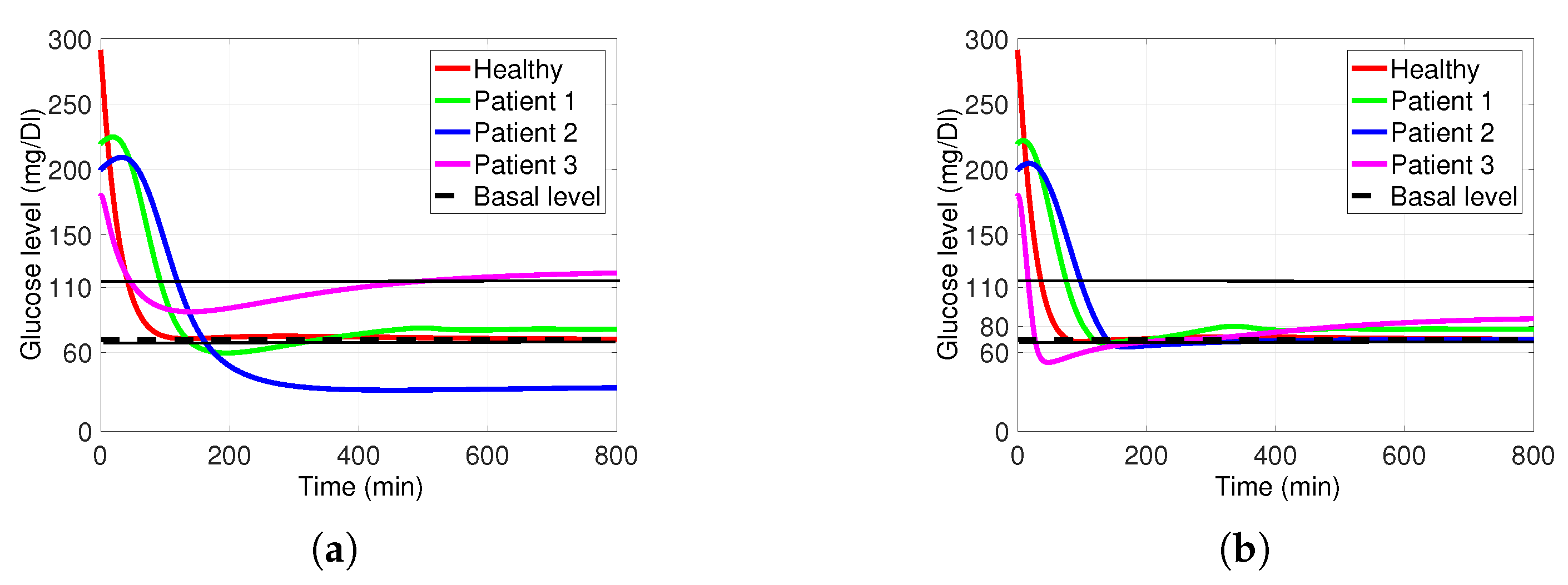
Figure 2a pictures the open-loop system response (1)–(4) with u ( t ) = 0 . Figure 2b presents the signal output of the closed-loop system (2)–(5) with the commuted PD controls (9) and (10) showing the effectiveness of the proposed commuted PD controller. Also, a comparison is presented in Figure 3, where the behavior of classic PD control [11] does not perform better than the proposed control strategy. Furthermore, the commuted PD controller stabilizes the blood glucose concentration at the basal value G b in the three cases. As Figure 3 shows, no hypoglycemia is attained when commuted PD control (9) and (10) is chosen. That is not the case when u g ( t ) (10) is not considered, as u c ( t ) behavior shows. In Figure 3c, considering commuted controller, in just a few minutes, hypoglycemia occurs. Then, the blood glucose concentration is normalized, but the basal glucose concentration is not reached.
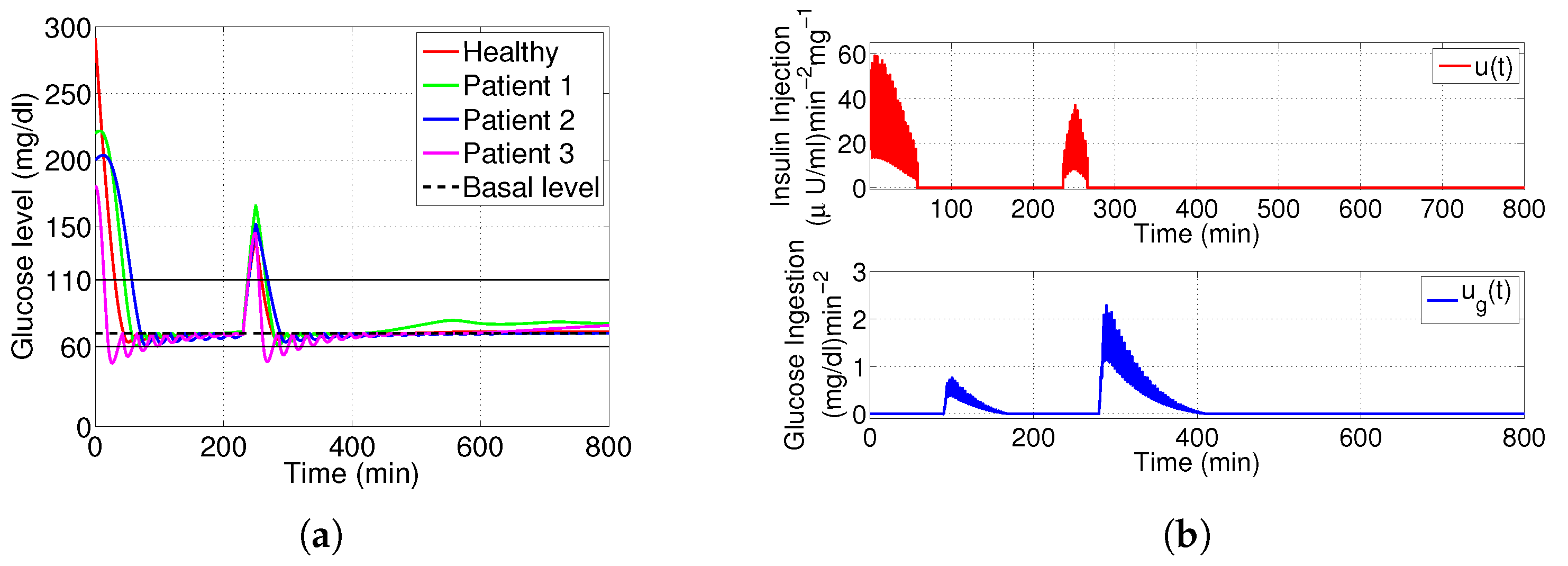
Figure 2. From (a), we notice that Patient 2 presents strong hypoglycemia (reaching 30 mg/dL), and Patient 3 hyperglycemia (reaching 120 mg/dL). From the closed-loop system (b), only Patient 3 presents hypoglycemia for one hour approximately, reaching the lowest glucose level 52 mg/dL (considered healthy in [4]). (a) Open-loop system (1)–(4). (b) Closed-loop system (2)–(5), with control (9) and (10).
Applsci 13 08129 g002
Figure 3. Closed-loop simulations. Classic model (16)–(18) with u c ( t ) (19) from [11], is compared to proposed system (2)–(5) with commuted PD controller (9) and (10). It shows how under the commuted PD controller (9) and (10) the glucose blood concentration is stabilized at G b . (a) Patient 1. (b) Patient 2. (c) Patient 3.
Applsci 13 08129 g003
Figure 4. Control input u ( t ) (9) and u g ( t ) (10), with D ( t ) defined in (4), for each patient under study. To prevent hypoglycemia, after a few minutes of the end of its injection, glucose ingestion is needed. (a) Patient 1. (b) Patient 2. (c) Patient 3.
Applsci 13 08129 g004
Analysing Figure 4, we see how commuted PD controller works. We comment on the Patient 1 case. During the first minutes after meal ingestion, when D ( t ) is biggest, the system needs insulin injection to reduce the glucose concentration (graphic of u ( t ) in Figure 4a). To normalize its level, glucose ingestion is needed an hour after (graphic of u g ( t ) in Figure 4a). This is a common situation difficult to deal with. This might indicate that the insulin administration could be too strong for a pancreatic system. To mitigate this effect, we suggest ingesting some controlled quantity of glucose. This is done by u g ( t ) (10) action. The same can be seen for Patients 2 and 3 given in Figure 4b and Figure 4c, respectively.

3.2. External Noise Perturbation

Now, an ingestion is considered an external disturbance. So, an intake meal at 230 min is introduced, after the controller is activated. It corresponds to the case of additive perturbation on (1) or (5), and defined as:
w ( t ) = 5 H ( t 230 ) H ( t 250 ) + A e B ( t 230 ) H ( t 230 ) ,
where the function H ( t a ) is the well-known Heaviside expression:
H ( t a ) = 0 t < a 1 t a .
Due to the additional glucose ingestion, an additional rate of glucose absorption has to be considered (exponential function in (20)). Hence, the classic mathematical model of the pancreatic system is given by [11]:
x ˙ 1 ( t ) = p 1 ( x 1 ( t ) G b ) x 1 ( t ) · x 2 ( t ) + D ( t ) + w ( t ) ,
x ˙ 2 ( t ) = p 2 x 2 ( t ) + p 3 ( x 3 ( t ) I b ) ,
x ˙ 3 ( t ) = n ( x 3 ( t ) I b ) + γ [ x 1 ( t ) σ ] + t + u c ( t ) ,
which, modified to our controlled system, results in:
x ˙ 1 ( t ) = p 1 ( x 1 ( t ) G b ) x 1 ( t ) · x 2 ( t ) + D ( t ) + u g ( t ) + w ( t ) ,
x ˙ 2 ( t ) = p 2 x 2 ( t ) + p 3 ( x 3 ( t ) I b ) ,
x ˙ 3 ( t ) = n ( x 3 ( t ) I b ) + γ [ x 1 ( t ) σ ] + t + u ( t ) ,
with u ( t ) defined in (9) and u g ( t ) in (10).
Figure 5 and Figure 6 present the simulations of Patients 1, 2, and 3 under the commuted PD controller action. In these cases, the commuted PD controller has a good performance, because no hypoglycemia range is attained. Hyperglycemia is attained only during ingestion, as expected.
Figure 5. Simulations of closed-loop system with external perturbation (20). The proposed control strategy performs better than PD control u c ( t )  [11], noticing that glucose ingestion is needed to prevent hypoglycemia episodes. (a) System (24)–(26) with the commuted PD controller (9) and (10). (b) System (21)–(23) with the PD controller u c ( t ) (19) in [11].
Applsci 13 08129 g005
Figure 6. Commuted PD controller (9) and (10), under external perturbation (20). Notice that the glucose ingestion suggested is small compared with the glucose blood concentration. (a) Patient 1. (b) Patient 2. (c) Patient 3.
Applsci 13 08129 g006

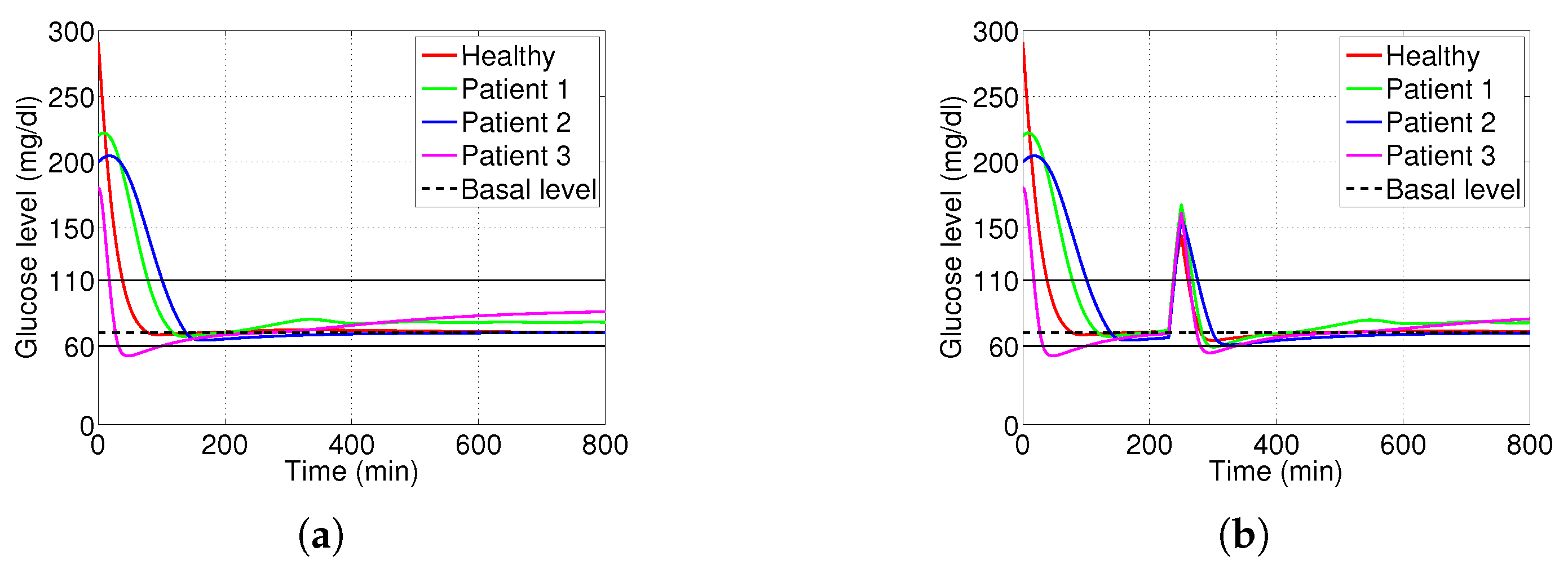
3.3. Changes on Glucose Assimilation

Consider a more general case to system in (5), where the dynamic of x 1 ( t ) is modified using an auxiliary variable x a ( t ) with an stable dynamic (27) and (28):
x ˙ 1 ( t ) = p 1 ( x 1 ( t ) G b ) x 1 ( t ) · x 2 ( t ) + D ( t ) + x a ( t ) ,
x ˙ a ( t ) = α x a ( t ) u g ( t ) .
The change on the dynamic assimilation smooths the control term, that is, we consider now that the insulin administration is slowed down, but the total level administration does not change. We set α = 2 . Figure 7 presents the simulations, where it can be noticed that its behavior is similar to (5). So, we can conclude that our control algorithm is robust against changes in patient dynamics for glucose assimilation.
Figure 7. Simulations of closed-loop system with commuted PD controller (9) and (10) when dynamical changes on the glucose assimilation are considered (27) and (28). Two comparative situations: (a) with w ( t ) = 0 and (b) under external perturbation (20). The behavior is similar to commuted model (5), as Figure 2b and Figure 5a show. (a) Unperturbed modified system (27) and (28). (b) Perturbed modified system (27) and (28) with w ( t ) 0 (20).
Applsci 13 08129 g007

3.4. PID Using Reset Integrator

As was mentioned in the introduction, we noticed from simulations that strong hypoglycemia occurs during a long period of time when the integral part of the PD controller is considered. In order to complete the study of the proposed switched strategy, we consider now a reset integral part. Hence, defining a commuted PID controller as:
u P I D ( t ) = k 1 x 1 ( t ) G b + k 2 x ˙ 1 ( t ) + k 3 0 t x 1 ( τ ) G b d τ .
That is, control (8) is now modified by the integral part with parameter k 3 . This term accounts for past values of the error between the desired glucose concentration G b and the actual glucose blood level. The limitations of the linear integrator can be faced using a reset integrator, also named as Clegg integrator [26]. This integrator resets its output to zero whenever its input and output have different signs [27,28]. Due to this resetting condition, the transient response of the controller can be arranged. Figure 8 captures the Matlab Simulink model used to compute the numerical simulation experiments. Based on Clegg integrator [26], we define a reset integrator block by taking into account that we need to integrate the error and to vanish it. Then, from Figure 8, we set:
  • Clegg integrator input. The error between glucose blood concentration x 1 ( t ) and the nominal value G b .
  • Clegg integrator initial condition. After each reset to the Clegg integrator, an initial condition is needed to integrate each resetting action. We use the zero initial condition setting.
  • Clegg integrator resetting actions. The block can reset its state to the specified initial condition based on an external signal. We choose to reset the integrator when the sinus function changes its sign.
  • Clegg integrator gain. The parameter k 3 = 0.1 is found by the trial and error method.
Figure 8. Matlab Simulink diagram block model used to study the behavior of the proposed control strategy to our pancreatic plant, considering reset integrator (29). When k 3 = 0 , we obtain the commuted PD controller (9) and (10). As a resetting signal, we use a sinusoidal function r ( t ) = sin ( t ) , and zero initial condition.
Applsci 13 08129 g008
Figure 9 shows the behavior of the commuted PID controller (29), where the rise time is reduced to 10 min approximately. But the controller presents chattering in all cases (we picture Patient 1 in Figure 9b as an example), and the insulin injection rate is increased.
Figure 9. Simulations of closed-loop system with external perturbation (20), using PID with reset integrator (29). The rise time is reduced to 10 min approximately compared to Figure 5a, but the control laws present chattering. (a) Commuted PID—External Perturbation w ( t ) (20). (b) Commuted PID controller (9) and (10) using (29), for Patient 1.
Applsci 13 08129 g009

4. Discussion of Results

A closed-loop artificial pancreas would measure glucose blood concentration, determine the expected time course following insulin administration, and dispense the optimal dose [36,37,38,39]. Our proposal seeks to do so by designing a commuted linear control able to keep the blood sugar concentration in a healthy region in terms of reducing the error between the actual glucose concentration and the desired one. To compare our strategy, we consider the reference [11] due to its similarity. As was remarked in the introduction, there are many results on the insulin–glucose regulation system, and we choose the Bergman model because is commonly used for diabetic systems. As was presented in Section 3, our approach shows better performance, surely due to two main reasons: (a) the glucose level alerts when hypoglycemia occurs (not considered in [11] or [16], for instance); (b) and the error between the glucose level and the desired setting is reduced. In fact, despite this, our control approach can be considered as an applied mathematics study, where its application is easy to understand. Additionally, the proportional factor in our control design tries to reduce the error signal, but the parameter k 1 in (8) must be tuned carefully. But once it is set, the controller must be able to face different patients’ biological uncertainties. On the other hand, the derivative factor of the controller regulates the rate of the changing error signal, which is mainly governed by parameter k 2 in (8). That is, it governs the future value of glucose concentration in terms of the present measurement (anticipatory control). Furthermore, if a white noise is present in the blood glucose measurement, our control strategy maintains healthy behavior, but the rise time is increased (see Figure 10). Only for the case of persistent hypoglycemia (Patient 2) the controller does not accomplish its purpose. In this case, the strategy must be different, maybe by considering a saturation effect on the insulin administration to avoid hypoglycemic episodes.

5. Conclusions and Future Work

This paper proposes a new strategy to control the blood glucose concentration in a pancreatic system, and with the control objective to reduce the error between this concentration with respect to the basal one. As is well-known, the main idea is to administrate insulin to prevent hyperglycemia. But this insulin dose could be too strong, falling into the hypoglycemia region. To mitigate this effect, we suggest ingesting some controlled quantity of glucose. The method used to define the controllers is the proportional-derivative one, which is able to stabilize the glucose concentration around its basal value. The key feature is to avoid an unhealthy glucose concentration range, combining insulin injection with glucose administration. Then, two control actions are defined: one to modify the insulin dynamics (and prevent hyperglycemia), and the other one to improve the performance of the glucose dynamics (and prevent hypoglycemia).
The simulations test the closed-loop performance on four different human behaviors. Moreover, external perturbations are considered meal ingestion. The results are comparable or improved with respect to other works. The purpose of this work is to study the behavior of this novel strategy, and opens the possibility of testing this switched strategy on another type of controller. Also, as theoretical future work, discontinuities of state variables can be considered by working with a piecewise smooth differential system. Moreover, the time delays in insulin administration can be also an interesting case to study [40].
Finally, two complementary studies are presented. One is based on modifying the glucose absorption dynamic, to test the robustness of the commuted PD controller. The other study was to include an integral part of our controller approach, defining a PID with a resetting integrator action, showing that despite the rise-time of closed-loop dynamics being reduced, chattering on the controller appears inevitably.

Author Contributions

Conceptualization, L.A.; Methodology, G.P.-V., L.A. and J.G.-B.; Software, G.P.-V.; Validation, G.P.-V., L.A. and J.G.-B.; Formal analysis, G.P.-V. and L.A.; Investigation, L.A.; Data curation, J.G.-B.; Writing—original draft, G.P.-V. and L.A.; Writing—review & editing, J.G.-B.; Visualization, L.A. and J.G.-B.; Supervision, G.P.-V. All authors have read and agreed to the published version of the manuscript.

Funding

This research received no external funding.

Institutional Review Board Statement

Not applicable.

Informed Consent Statement

Not applicable.

Data Availability Statement

No data were created during the study.

Conflicts of Interest

The authors declare no conflict of interest.

Appendix A

In this appendix, we check the stability conditions established in Section 2.4 without external disturbances, that is, considering D ( t ) = 0 . We apply Filippov’s theory [31,32,33], where a vector solution x ( t ) in (12) is said to exist if it is absolutely continuous on [ 0 , ) , and for almost all t [ 0 , ) , if x ˙ belongs to the convex closure over all sets of measure zero. Moreover, a system (12) is quadratically stable if there exist Lyapunov functions V j = V j ( t , x ) , j = 1 , 2 , verifying two conditions [32]:
(i)
x R 3 { s j } : V j ˙ < 0 ,
(ii)
x { s j } : sup α [ 0 , 1 ] V i x α f 0 ( t , x ) + ( 1 α ) f j ( t , x ) < 0 .
First, and only for stability proof, we use Jacobian linearization to linearize the nonlinear system (12) around the equilibrium point ( G b , 0 , I b ) :
f ¯ 1 = p 1 k 1 1 k 2 G b 0 0 p 2 p 3 0 0 n
f ¯ 0 = p 1 G b 0 0 p 2 p 3 0 0 n
f ¯ 2 = p 1 G b 0 0 p 2 p 3 k 1 p 1 k 2 k 2 G b n
The existence of the Lyapunov function of condition (i) from Filippov’s theory is ensured by the negativeness of the eigenvalues of the matrices (A1)–(A3) from the linearized model. Hence, from the triangular expression of (A2) the negativeness is obvious. The eigenvalues of (A1) have negative real part if p 1 k 1 1 k 2 < 0 , where p 1 > 0 . Hence, these inequalities define a condition on the PD-control parameters:
p 1 k 1 1 k 2 < 0 p 1 + k 1 1 k 2 > 0 k 2 < 1 .
Under assumption k 2 < 1 , the stability of (A3) is verified, and the existence of Lyapunov function V j is guaranteed if k 1 < n · p 2 G b · p 3 . From the experimental data in Table 1, we obtain k 1 < 0.301 . Condition (ii) ensures the stability where x 1 takes its critical value.
It is worthy to comment on the case of a discontinuity in x 2 , or x 3 in (5)–(7). This would make the Filippov treatment a higher co-dimensional problem. Our control approach is based on the sign of x 1 to activate the corresponding controller block. Therefore, if a discontinuity appears on variables x 2 or x 3 , the control law can not be modified because only the glucose level is measured, but the stability issue is drastically increased [41]. One option to resolve this is to establish a safety region for variable x 3 , where the insulin concentration is considered healthy (from a physiologic point of view, we can consider I b ± ϵ , with ϵ view as a measurement error). So, two intersecting smooth manifolds of co-dimension 1 define three regions on x 1 , and another two manifolds define the x 3 ’s regions. Then, R 2 is divided into nine regions, where condition (ii) must be verified in each one. This study is not treated here, but it is an interesting theoretical issue for future work.

References

  1. Nwokolo, M.; Hovorka, R. The Artificial Pancreas and Type 1 Diabetes. J. Clin. Endocrinol. Metab. 2023, 108, 1614–1623. [Google Scholar] [CrossRef]
  2. Carson, E.R.; Deutsch, T. A Spectrum of approaches for controlling diabetes. IEEE Control Syst. Mag. 1992, 12, 25–31. [Google Scholar]
  3. Cobelli, C.; Dalla Man, C.; Sparacino, G.; Magni, L.; De Nicolao, G.; Kovatchev, B.P. Diabetes: Models, Signals, and Control. IEEE Rev. Biomed. Eng. 2009, 2, 54–96. [Google Scholar] [CrossRef] [PubMed] [Green Version]
  4. Dua, P.; Doyle, F.J., III; Pistikopoulos, E.N. Model-based glucose control for Type-1 diabetes via parametric programming. IEEE Trans. Biomed. Eng. 2006, 53, 1478–1491. [Google Scholar] [CrossRef] [PubMed]
  5. Chee, F.; Savkin, A.V.; Fernando, T.L.; Nahavandi, S. Optimal H insulin injection control for blood glucose regulation in diabetic patients. IEEE Trans. Biomed. Eng. 2005, 52, 1625–1631. [Google Scholar] [CrossRef]
  6. Kaveh, P.; Shtessel, Y.B. Blood glucose regulation using higher-order sliding mode control. Int. J. Robust Nonlinear Control 2008, 18, 557–569. [Google Scholar] [CrossRef]
  7. Leon, B.S.; Alanis, A.Y.; Sanchez, E.N.; Ornelas-Tellez, F.; Ruiz-Velazquez, E. Inverse optimal neural control of blood glucose level for type 1 diabetes mellitus patients. J. Frankl. Inst. 2012, 349, 1851–1870. [Google Scholar] [CrossRef]
  8. El Fathi, A.; Smaoui, M.R.; Gingras, V.; Boulet, B.; Haidar, A. The Artificial Pancreas and Meal Control: An Overview of Postprandial Glucose Regulation in Type 1 Diabetes. IEEE Control Syst. 2018, 38, 67–85. [Google Scholar]
  9. Makroglou, A.; Li, J.; Kuang, Y. Mathematical models and software tools for the glucose-insulin regulatory system and diabetes: An overview. Appl. Numer. Math. 2006, 56, 559–573. [Google Scholar] [CrossRef]
  10. Hernjak, N.; Doyle, F.J., III. Glucose control design using nonlinearity assessment techniques. AIChE J. 2005, 51, 544–554. [Google Scholar] [CrossRef]
  11. Li, C.; Hu, R. Simulation study on blood glucose control in diabetics. In Proceedings of the 2007 1st International Conference on Bioinformatics and Biomedical Engineering, Wuhan, China, 6–8 July 2007. [Google Scholar]
  12. Amuthameena, S. A novel strategy for blood glucose control in human body using PID-Fuzzy logic controller. J. Chem. Pharm. Sci. 2016, 8, 88–92. [Google Scholar]
  13. Marchetti, G.; Barolo, M.; Jovanovic, L.; Zisser, H.; Seborg, D.E. An improved PID switching control strategy for Type 1 Diabetes. IEEE Trans. Biomed. Eng. 2008, 55, 857–865. [Google Scholar] [CrossRef]
  14. Hoyos, J.D.; Bolanos, F.; Vallejo, M.; Rivadeneira, P.S. Population-based incremental learning algorithm for identification of blood glucose dynamics model for type-1 diabetic patients. In Proceedings of the International Conference on Artificial Intelligence, Chengdu China, 12–14 March 2018; pp. 29–35. [Google Scholar]
  15. Villa Tamayo, M.F.; Caicedo Alvarez, M.A.; Rivadeneira, P.S. Handling Parameter Variations during the Treatment of Type 1 Diabetes Mellitus: In Silico Results. Math. Probl. Eng. 2019, 2019, 2640405. [Google Scholar] [CrossRef]
  16. Ndakara, A.I.; Essabbar, M.; Saikouk, H. Blood Glucose-Insulin Dynamics in Type-1 Diabetic Patients for the Mitigation of Hyperglycemic Conditions: A PID Controller with a Step Response. In Digital Technologies and Applications; Motahhir, S., Bossoufi, B., Eds.; ICDTA 2023; Lecture Notes in Networks and Systems; Springer: Cham, Switzerland, 2023; Volume 668. [Google Scholar]
  17. Syafiie, S.; AlHarbi, F.; Alshehri, A.A.; Hasanain, B. PID and LQG controllers for diabetes system with internal delay: A comparison study. Biomed. Phys. Eng. Express 2023, 9, 035031. [Google Scholar] [CrossRef]
  18. Kaveh, P.; Shtessel, Y.B. Blood Glucose Regulation in Diabetics Using Sliding Mode Control Techniques. In Proceedings of the Thirty-Eighth Southeastern Symposium on System Theory, Cookeville, TN, USA, 5–7 March 2006. [Google Scholar]
  19. De Gaetano, A.; Arino, O. Mathematical modelling of the intravenous glucose tolerance test. J. Math. Biol. 2000, 40, 136–168. [Google Scholar] [CrossRef]
  20. Fisher, M.E. A semiclosed-loop algorithm for the control of blood glucose levels in diabetics. IEEE Trans. Biomed. Eng. 1991, 38, 57–61. [Google Scholar] [CrossRef]
  21. Colmegna, P.H.; Sanchez-Pena, R.S.; Gondhalekar, R.; Dassau, E.; Doyle, F.J. Switched LPV Glucose Control in Type 1 Diabetes. IEEE Trans. Biomed. Eng. 2016, 63, 1192–1200. [Google Scholar] [CrossRef] [Green Version]
  22. Batmani, Y. Blood glucose concentration control for type 1 diabetic patients: A non-linear suboptimal approach. IET Syst. Biol. 2017, 11, 119–125. [Google Scholar] [CrossRef]
  23. Messori, M.; Incremona, G.P.; Cobelli, C.; Magni, L. Individualised model predictive control for the artificial pancreas: In Silico evaluation of closed-loop glucose control. IEEE Control Syst. 2018, 38, 86–104. [Google Scholar]
  24. Ankit Sharma, N.; Singh, H.P. Computer-controlled diabetes disease diagnosis technique based on fuzzy inference structure for insulin-dependent patients. Appl. Intell. 2023, 53, 1945–1958. [Google Scholar] [CrossRef]
  25. Emerson, H.; Guy, M.; McConville, R. Offline reinforcement learning for safer blood glucose control in people with type 1 diabetes. J. Biomed. Inform. 2023, 142, 104376. [Google Scholar] [CrossRef] [PubMed]
  26. Clegg, J.C. A nonlinear integrator for servomechanism. Trans. Am. Inst. Electr. Eng. Part II Appl. Ind. 1958, 77, 41–42. [Google Scholar] [CrossRef]
  27. Nesic, D.; Zaccarian, L.; Teel, A.R. Stability properties of reset systems. IFAC Proc. Vol. 2005, 38, 67–72. [Google Scholar] [CrossRef]
  28. Banos, A.; Barreiro, A. Reset Control Systems; Springer Sciences and Business Media: London, UK, 2011. [Google Scholar]
  29. Palumbo, P.; Ditlevsen, S.; Bertuzzi, A.; De Gaetano, A. Mathematical modeling of glucose-insulin system: A review. Math. Biosci. 2013, 244, 69–81. [Google Scholar] [CrossRef]
  30. Bergman, R.N.; Phillips, L.S.; Cobelli, C. Physiologic evaluation of factors controlling glucose tolerance in man: Measurement of insulin sensitivity and beta-cell glucose sensitivity from the response to intravenous glucose. J. Clin. Investig. 1981, 68, 1456–1467. [Google Scholar] [CrossRef] [Green Version]
  31. Filippov, A.F. Differential Equations with Discontinuous Right-Hand Sides; Kluwer Academic: Boston, MA, USA, 1988. [Google Scholar]
  32. Frankowska, H. Filippov’s and Filippov-Wazewski’s theorems on closed domains. J. Differ. Equ. 2000, 161, 449–478. [Google Scholar] [CrossRef]
  33. Dieci, L.; Lopez, L. Sliding motion in Filippov differential systems: Theoretical results and a computational approach. SIAM J. Numer. Anal. 2009, 47, 2023–2051. [Google Scholar] [CrossRef] [Green Version]
  34. Gena, P.; Del Buono, N.; D’Abbicco, M.; Mastrodonato, M.; Berardi, M.; Svelto, M.; Lopez, L.; Calamita, G. Calamita, Dynamical modeling of liver Aquaporin-9 expression and glycerol permeability in hepatic glucose metabolism. Eur. J. Cell Biol. 2017, 96, 61–69. [Google Scholar] [CrossRef]
  35. Ang, K.H.; Chong, G.; Li, Y. PID control system analysis, design, and technology. IEEE Trans. Control Syst. Technol. 2005, 13, 559–576. [Google Scholar]
  36. León-Vargas, F.; Garelli, F.; De Battista, H.; Vehí, J. Postprandial response improvement via safety layer in closed-loop blood glucose controllers. Biomed. Signal Process. Control 2015, 16, 80–87. [Google Scholar] [CrossRef]
  37. Rossetti, P.; Quiros, C.; Moscardo, V.; Comas, A.; Giménez, M.; Ampudia-Blasco, F.J.; León, F.; Montaser, E.; Conget, I.; Bondia, J.; et al. Closed-Loop Control of Postprandial Glycemia Using an Insulin-on-Board Limitation Through Continuous Action on Glucose Target. Diabetes Technol. Ther. 2017, 19, 355–362. [Google Scholar] [CrossRef]
  38. Boiroux, D.; Duun-Henriksen, A.K.; Schmidt, S.; Nørgaard, K.; Poulsen, N.K.; Madsen, H.; Jørgensen, J.B. Adaptive control in an artificial pancreas for people with type 1 diabetes. Control Eng. Pract. 2017, 58, 332–342. [Google Scholar] [CrossRef]
  39. Glass, L. Dynamical disease: Challenges for nonlinear dynamics and medicine. Chaos 2015, 25, 097603. [Google Scholar] [CrossRef]
  40. Tunç, C. Stability and bounded of solutions to non-autonomous delay differential equations of third order. Nonlinear Dyn. 2010, 62, 945–953. [Google Scholar] [CrossRef]
  41. Difonzo, F.V. A note on attractivity for the intersection of two discontinuity manifolds. Opusc. Math. 2020, 40, 685–702. [Google Scholar] [CrossRef]
Figure 1. Block diagram of the closed-loop controlled system of insulin-dependent diabetic patients. A sensor measures the glucose blood concentration and compares it to the reference value (normal glucose level). Then, the control algorithm decides the amount of insulin administration delivered to the patient through a pump.
Applsci 13 08129 g001
Figure 10. White noise on measurements. In this case, white noise is considered to simulate a worse case of glucose measurement error. It is observed that the controller regulates the glucose concentration to a healthy one of 70 mg/dL, but slower than without error measurements. Hence, for this noise environment, if external ingestion occurs, almost all patients cases are regulated, except case 2 (hypoglycemic patient). (a) Without external perturbation. (b) With ingestion at 230–250 min.
Applsci 13 08129 g010
Table 1. Parameter values [6]. The value * in Patient 3 denotes a modified value to obtain a notable hyperglycemia case.
HealthyPatient 1Patient 2Patient 3
p 1 0.0317000
p 2 0.01230.020.00720.0142
p 3 4.92 × 10 6 5.3 × 10 6 2.16 × 10 6 9.94 × 10 5
γ 0.00390.0050.00380.0 *
n0.26590.30.24650.2814
σ 79.03537877.578382.9370
G b 70707070
I b 7777
x 1 ( 0 ) 291.2220200180
x 2 ( 0 ) 0000
x 3 ( 0 ) 364.8505560
Disclaimer/Publisher’s Note: The statements, opinions and data contained in all publications are solely those of the individual author(s) and contributor(s) and not of MDPI and/or the editor(s). MDPI and/or the editor(s) disclaim responsibility for any injury to people or property resulting from any ideas, methods, instructions or products referred to in the content.

