
Model-Free Adaptive Nonsingular Fast Integral Terminal Sliding Mode Control for Wastewater Treatment Plants


Abstract
:1. Introduction
- (1)
- The proposed method does not rely on the mathematical model or human experience of WWTP and only requires real-time I/O measurement data. It can effectively avoid the uncertainty of the model and the impact of unmodeled dynamics on the closed-loop system.
- (2)
- A novel fast integral terminal sliding mode surface (FITSMS) is proposed to ensure that the tracking error can converge quickly when it is far from the equilibrium point. This addresses the issue that the conventional integral sliding mode control (ISMC) cannot ensure that the system state convergences to zero in a finite time and the rate of convergence of the tracking error is slow.
- (3)
- The BSM1 was used to validate the suggested approach’s control performance and it was contrasted with other control schemes including PID and MPC. The simulation experiment results indicate that the MFA-NFITSMC strategy has a better tracking performance and stronger robustness in the control of WWTP.
2. Problem Description
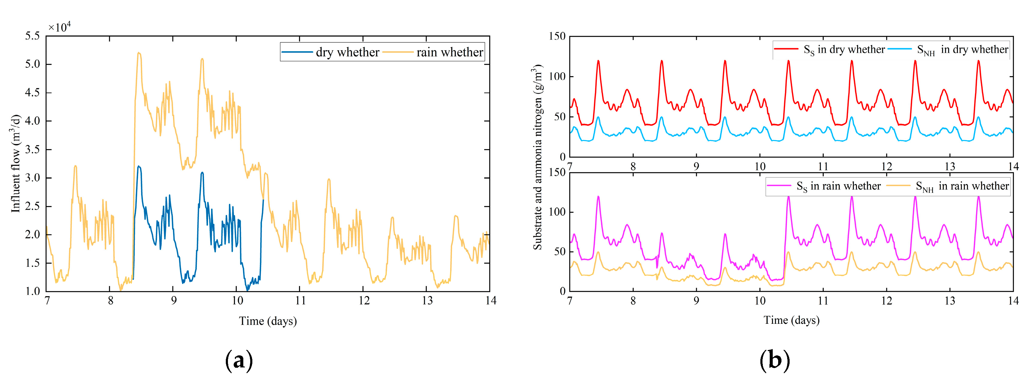
2.1. Benchmark Simulation Model No. 1 (BSM1)
2.2. CFDL Model for WWTP
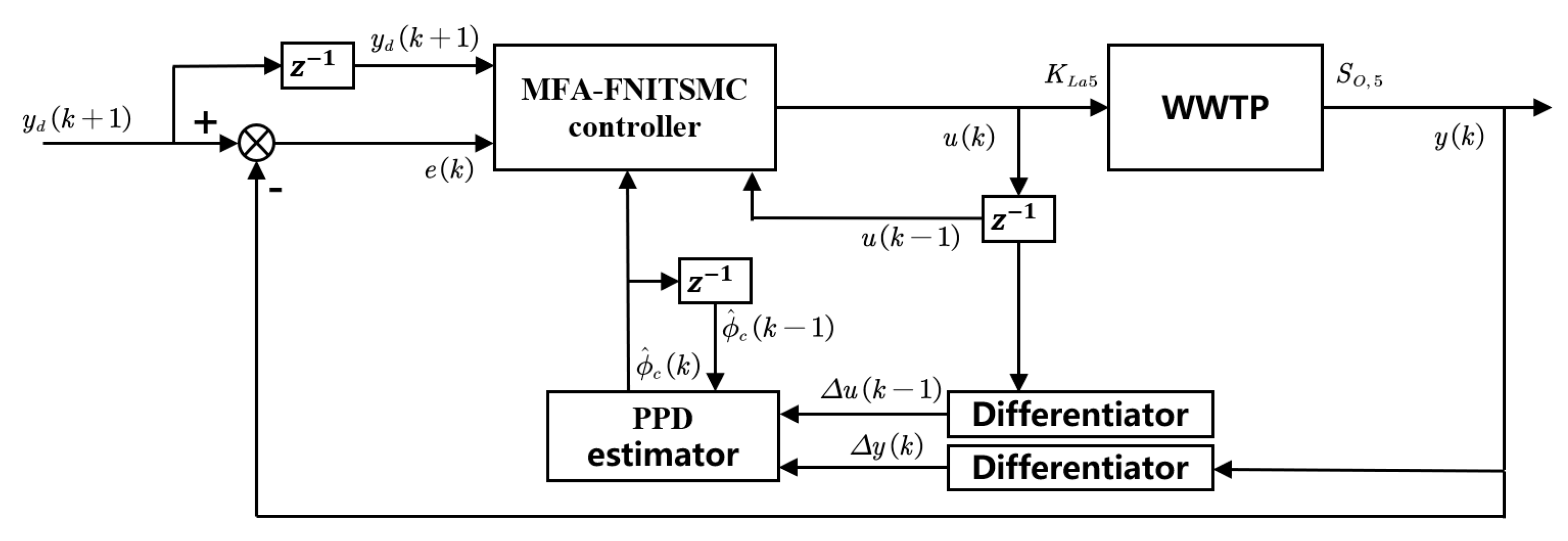
3. Controller Design for WWTP
3.1. Fast Integral Terminal Sliding Mode Surface
3.2. MFA-NFITSMC Design
3.3. Stability Analysis
- (1)
- The WWTP system’s tracking error is convergent., and .
- (2)
- The output and input sequences and are bounded.
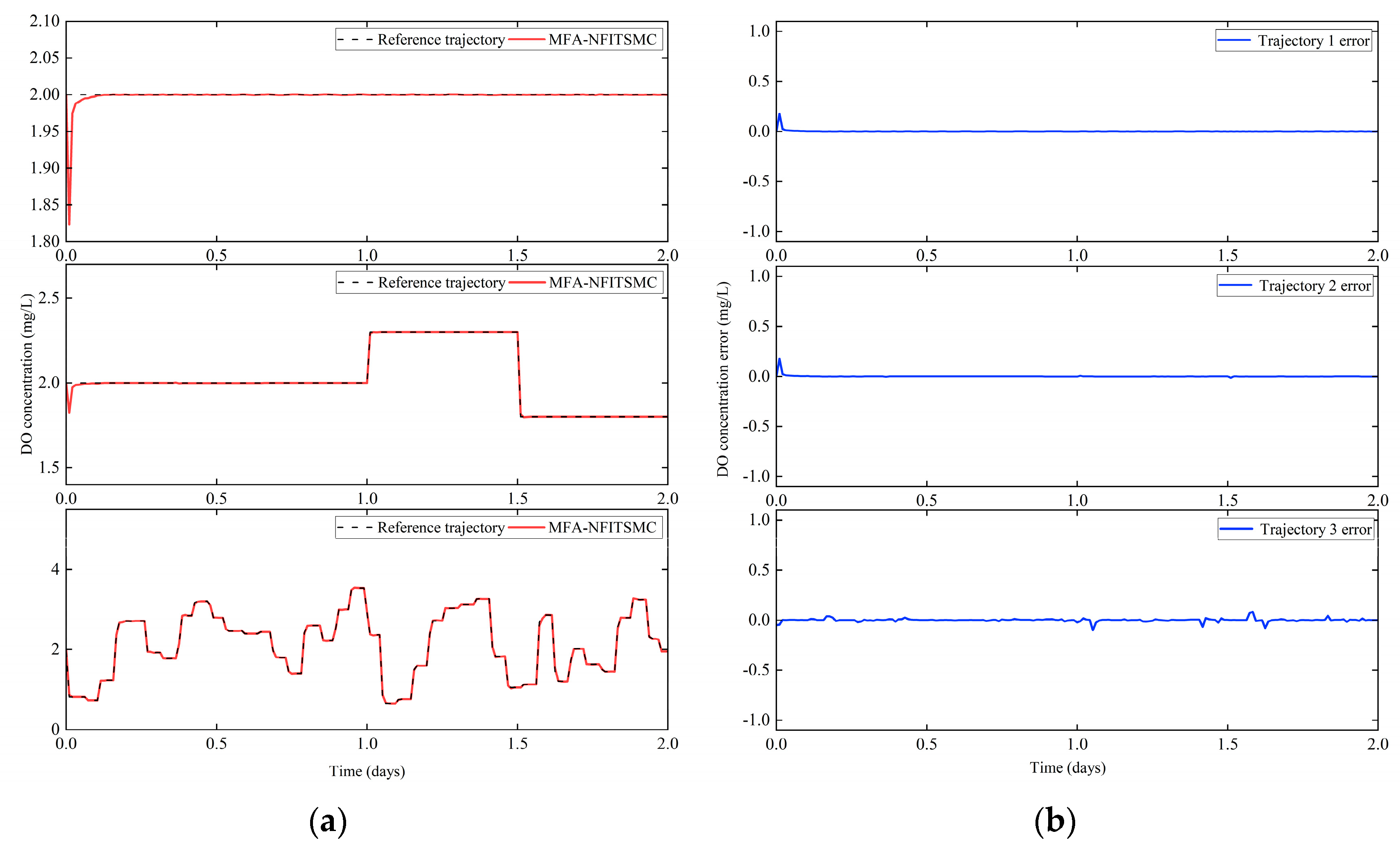
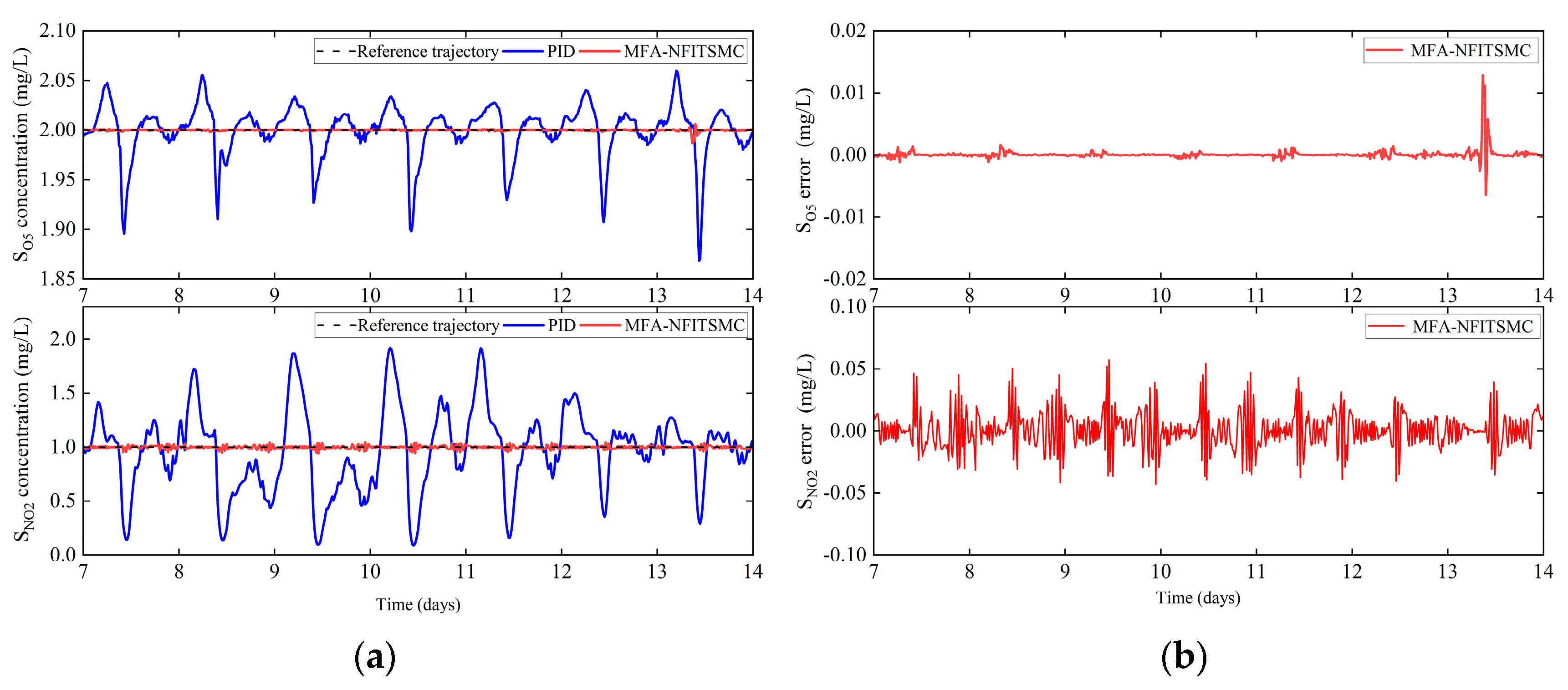
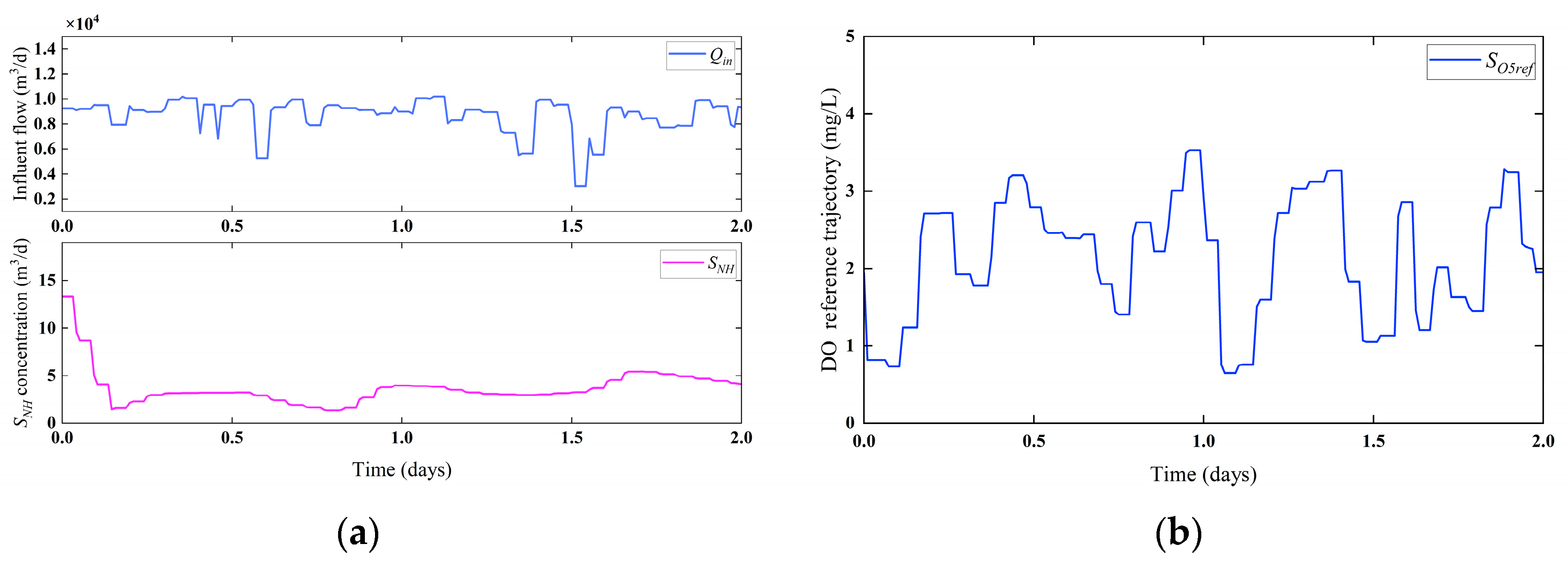
4. Simulation
5. Conclusions
Author Contributions
Funding
Data Availability Statement
Acknowledgments
Conflicts of Interest
References
- The Cost Simulation Benchmark-Description and Simulator Manual; Office for Publications of the European Community: Luxembourg, 2001.
- Suescun, J.; Irizar, I.; Ostolaza, X.; Ayesa, E. Dissolved oxygen control and simultaneous estimation of oxygen uptake rate in activated-sludge plants. Water Environ. Res. 1998, 70, 316–322. [Google Scholar] [CrossRef]
- Wahab, N.A.; Katebi, R.; Balderud, J. Multivariable PID control design for activated sludge process with nitrification and denitrification. Biochem. Eng. J. 2009, 45, 239–248. [Google Scholar] [CrossRef]
- Ferrer, J.; Rodrigo, M.A.; Seco, A.; Penya-Roja, J.M. Energy saving in the aeration process by fuzzy logic control. Water Sci. Technol. 1998, 38, 209–217. [Google Scholar] [CrossRef]
- Traore, A.; Grieu, S.; Puig, S.; Corominas, L.; Thiéry, F.; Polit, M.; Colprim, J. Fuzzy control of dissolved oxygen in a sequencing batch reactor pilot plant. Chem. Eng. J. 2005, 111, 13–19. [Google Scholar] [CrossRef]
- Zhu, G.; Peng, Y.; Ma, B.; Wang, Y.; Yin, C. Optimization of anoxic/oxic step feeding activated sludge process with fuzzy control model for improving nitrogen removal. Chem. Eng. J. 2009, 151, 195–201. [Google Scholar] [CrossRef]
- Holenda, B.; Domokos, E.; Redey, A.; Fazakas, J. Dissolved oxygen control of the activated sludge wastewater treatment process using model predictive control. Comput. Chem. Eng. 2008, 32, 1270–1278. [Google Scholar] [CrossRef]
- Dominic, S.; Shardt, Y.A.; Ding, S.X.; Luo, H. An adaptive, advanced control strategy for KPI-based optimization of industrial processes. IEEE Trans. Ind. Electron. 2015, 63, 3252–3260. [Google Scholar] [CrossRef]
- Han, H.G.; Qin, C.H.; Sun, H.Y.; Qiao, J.F. Adaptive sliding mode control for municipal wastewater treatment process. Acta Autom. Sin. 2023, 49, 1010–1018. [Google Scholar]
- Qiao, J.F.; Han, G.; Han, H.G. Neural network on-line modeling and controlling method for multi-variable control of wastewater treatment processes. Asian J. Control 2014, 16, 1213–1223. [Google Scholar] [CrossRef]
- Qiao, J.F.; Hou, Y.; Zhang, L.; Han, H.G. Adaptive fuzzy neural network control of wastewater treatment process with multiobjective operation. Neurocomputing 2018, 275, 383–393. [Google Scholar] [CrossRef]
- Han, H.G.; Qiao, J.F.; Chen, Q.L. Model predictive control of dissolved oxygen concentration based on a self-organizing RBF neural network. Control Eng. Pract. 2012, 20, 465–476. [Google Scholar] [CrossRef]
- Han, H.G.; Wu, X.L.; Qiao, J.F. Real-time model predictive control using a self-organizing neural network. IEEE Trans. Neural Netw. Learn. Syst. 2013, 24, 1425–1436. [Google Scholar] [PubMed]
- Han, H.; Qiao, J. Nonlinear model-predictive control for industrial processes: An application to wastewater treatment process. IEEE Trans. Ind. Electron. 2013, 61, 1970–1982. [Google Scholar] [CrossRef]
- Han, H.G.; Zhang, L.; Hou, Y.; Qiao, J.F. Nonlinear model predictive control based on a self-organizing recurrent neural network. IEEE Trans. Neural Netw. Learn. Syst. 2015, 27, 402–415. [Google Scholar] [CrossRef] [PubMed]
- Hou, Z.S.; Wang, Z. From model-based control to data-driven control: Survey, classification and perspective. Inf. Sci. 2013, 235, 3–35. [Google Scholar] [CrossRef]
- Hou, Z.; Jin, S. A novel data-driven control approach for a class of discrete-time nonlinear systems. IEEE Trans. Control Syst. Technol. 2010, 19, 1549–1558. [Google Scholar] [CrossRef]
- Xu, J.; Xu, F.; Wang, Y.; Sui, Z. An Improved Model-Free Adaptive Nonlinear Control and Its Automatic Application. Appl. Sci. 2023, 13, 9145. [Google Scholar] [CrossRef]
- Xu, D.; Jiang, B.; Liu, F. Improved data driven model free adaptive constrained control for a solid oxide fuel cell. IET Control Theory Appl. 2016, 10, 1412–1419. [Google Scholar] [CrossRef]
- Li, J.; Tang, Z.; Luan, H.; Liu, Z.; Xu, B.; Wang, Z.; He, W. An Improved Method of Model-Free Adaptive Predictive Control: A Case of pH Neutralization in WWTP. Processes 2023, 11, 1448. [Google Scholar] [CrossRef]
- Wang, Y.; Hou, M. Model-free adaptive integral terminal sliding mode predictive control for a class of discrete-time nonlinear systems. ISA Trans. 2019, 93, 209–217. [Google Scholar] [CrossRef]
- Esmaeili, B.; Salim, M.; Baradarannia, M. Predefined performance-based model-free adaptive fractional-order fast terminal sliding-mode control of MIMO nonlinear systems. ISA Trans. 2022, 131, 108–123. [Google Scholar] [CrossRef]
- Esmaeili, B.; Salim, M.; Baradarannia, M. Control of MIMO nonlinear discrete-time systems with input saturation via data-driven model-free adaptive fast terminal sliding mode controller. In Proceedings of the 2020 28th Iranian Conference on Electrical Engineering (ICEE), Tabriz, Iran, 4–6 August 2020. [Google Scholar]
- Alex, J.; Beteau, J.F.; Copp, J.B.; Hellinga, C.; Jeppsson, U.; Marsili-Libelli, S.; Vanhooren, H. Benchmark for evaluating control strategies in wastewater treatment plants. In Proceedings of the 1999 European Control Conference (ECC), Karlsruhe, Germany, 31 August—3 September 1999. [Google Scholar]
- Hou, Z.; Jin, S. Model Free Adaptive Control: Theory and Applications; CRC Press: Boca Raton, FL, USA, 2013. [Google Scholar]
- Chiu, C.S. Derivative and integral terminal sliding mode control for a class of MIMO nonlinear systems. Automatica 2012, 48, 316–326. [Google Scholar] [CrossRef]
- Xu, W.; Junejo, A.K.; Liu, Y.; Hussien, M.G.; Zhu, J. An efficient antidisturbance sliding-mode speed control method for PMSM drive systems. IEEE Trans. Power Electron. 2020, 36, 6879–6891. [Google Scholar] [CrossRef]
- Xu, Q.; Li, Y. Micro-/nanopositioning using model predictive output integral discrete sliding mode control. IEEE Trans. Ind. Electron. 2011, 59, 1161–1170. [Google Scholar] [CrossRef]
- Cao, W.; Yang, Q. Online sequential extreme learning machine based adaptive control for wastewater treatment plant. Neurocomputing 2020, 408, 169–175. [Google Scholar] [CrossRef]
- Vilanova, R.; Katebi, M.R.; Wahab, N. N-removal on wastewater treatment plants: A process control approach. J. Water Resour. Prot. 2011, 2011, 1–11. [Google Scholar] [CrossRef]
- Belchior, C.A.C.; Araújo, R.A.M.; Landeck, J.A.C. Dissolved oxygen control of the activated sludge wastewater treatment process using stable adaptive fuzzy control. Comput. Chem. Eng. 2012, 37, 152–162. [Google Scholar] [CrossRef]
- Du, X.; Wang, J.; Jegatheesan, V.; Shi, G. Dissolved Oxygen Control in Activated Sludge Process Using a Neural Network-Based Adaptive PID Algorithm. Appl. Sci. 2018, 8, 261. [Google Scholar] [CrossRef]


| Notation | Definition |
|---|---|
| Soluble inert organic matter | |
| Readily biodegradable substrate | |
| Particulate inert organic matter | |
| Slowly biodegradable substrate | |
| Active heterotrophic biomass | |
| Active autotrophic biomass | |
| Particulate products arising from biomass decay | |
| Oxygen | |
| Nitrate and nitrite nitrogen | |
| NH4+ + NH3 nitrogen | |
| Soluble biodegradable organic nitrogen | |
| Particulate biodegradable organic nitrogen | |
| Alkalinity |
| Control Strategy | ISE | IAE | |
|---|---|---|---|
| MFA-NFITSMC | 0.00014 | 0.0273 | 0.0083 |
| OS-ELM [29] | 0.00069 * | 0.0475 * | 0.0381 * |
| PI + AT [30] | 0.0009 * | 0.0490 * | - |
| AFC [31] | 0.0012 * | 0.0792 * | 0.0198 * |
| MPC [7] | 0.0026 * | 0.0890 * | 0.0781 * |
| BFC [31] | 0.0049 * | 0.1507 * | 0.0578 * |
| PID | 0.0078 | 0.1576 | 0.1425 |
| Control Strategy | ISE | IAE | |
|---|---|---|---|
| MFA-NFITSMC | 0.00014 | 0.0273 | 0.0083 |
| OS-ELM [29] | 0.00067 * | 0.0375 * | 0.0389 * |
| NNOMC [10] | 0.00053 * | 0.0390 * | - |
| SR-RBF [15] | - | 0.0630 * | - |
| RBFNNPID [32] | 0.0025 * | 0.0947 * | 0.0694 * |
| SORBF-MPC [12] | - | 0.0810 * | - |
| PID | 0.0045 | 0.1239 | 0.0952 |
| Reference Trajectory | ISE | IAE | |
|---|---|---|---|
| Trajectory 1 | 3.3604 × 10⁻⁴ | 0.0031 | 0.1768 |
| Trajectory 2 | 3.4848 × 10⁻⁴ | 0.0042 | 0.1768 |
| Trajectory 3 | 5.2901 × 10⁻⁴ | 0.0142 | 0.1004 |
| Control Strategy | ||||||
|---|---|---|---|---|---|---|
| ISE | IAE | ISE | IAE | |||
| MFA-NFITSMC | 0.00058 | 0.0013 | 0.0128 | 0.0016 | 0.0782 | 0.0571 |
| ASMC [9] | 0.00493 * | 0.035 * | 0.49 * | 0.00527 * | 0.046 * | 0.42 * |
| SMC [9] | 0.00552 * | 0.030 * | 0.61 * | 0.00562 * | 0.046 * | 0.44 * |
| PID | 0.0143 | 0.072 | 0.74 | 0.0081 | 0.056 | 0.53 |
Disclaimer/Publisher’s Note: The statements, opinions and data contained in all publications are solely those of the individual author(s) and contributor(s) and not of MDPI and/or the editor(s). MDPI and/or the editor(s) disclaim responsibility for any injury to people or property resulting from any ideas, methods, instructions or products referred to in the content. |
© 2023 by the authors. Licensee MDPI, Basel, Switzerland. This article is an open access article distributed under the terms and conditions of the Creative Commons Attribution (CC BY) license (https://creativecommons.org/licenses/by/4.0/).
Share and Cite
Xu, B.; Wang, Z.; Liu, Z.; Chen, Y.; Wang, Y. Model-Free Adaptive Nonsingular Fast Integral Terminal Sliding Mode Control for Wastewater Treatment Plants. Appl. Sci. 2023, 13, 13023. https://doi.org/10.3390/app132413023
Xu B, Wang Z, Liu Z, Chen Y, Wang Y. Model-Free Adaptive Nonsingular Fast Integral Terminal Sliding Mode Control for Wastewater Treatment Plants. Applied Sciences. 2023; 13(24):13023. https://doi.org/10.3390/app132413023
Chicago/Turabian StyleXu, Baochang, Zhongjun Wang, Zhongyao Liu, Yiqi Chen, and Yaxin Wang. 2023. "Model-Free Adaptive Nonsingular Fast Integral Terminal Sliding Mode Control for Wastewater Treatment Plants" Applied Sciences 13, no. 24: 13023. https://doi.org/10.3390/app132413023
APA StyleXu, B., Wang, Z., Liu, Z., Chen, Y., & Wang, Y. (2023). Model-Free Adaptive Nonsingular Fast Integral Terminal Sliding Mode Control for Wastewater Treatment Plants. Applied Sciences, 13(24), 13023. https://doi.org/10.3390/app132413023