Abstract
In the practical control of nonlinear valve systems, PID control, as a model-free method, continues to play a crucial role thanks to its simple structure and performance-oriented tuning process. To improve the control performance, advanced gain-scheduling methods are used to schedule the PID control gains based on the operating conditions and/or tracking error. However, determining the scheduled gain is a major challenge, as PID control gains need to be determined at each operating condition. In this paper, a model-assisted online optimization method is proposed based on the modified Non-Dominated Sorting Genetic Algorithms-II (NSGA-II) to obtain the optimal gain-scheduled PID controller. Model-assisted offline optimization through computer-in-the-loop simulation provides the initial scheduled gains for an online algorithm, which then uses the iterative NSGA-II algorithm to automatically schedule and tune PID gains by online searching of the parameter space. As a summary, the proposed approach presents a PID controller optimized through both model-assisted learning based on prior model knowledge and model-free online learning. The proposed approach is demonstrated in the case of a nonlinear valve system able to obtain optimal PID control gains with a given scheduled gain structure. The performance improvement of the optimized gain-scheduled PID control is demonstrated by comparing it with fixed-gain controllers under multiple operating conditions.
1. Introduction
For many valve actuation systems, designing a closed-loop valve position control system is challenging due to its nonlinear frictions, especially for valves that must operate in high temperature environments, such as exhaust gas recirculation (EGR) valves. One approach is to apply advanced model-based control strategies (for example, sliding mode control [1], linear parameter-varying control [2,3,4], etc.) to deal with valve system nonlinearity. However, it is difficult to obtain an accurate nonlinear friction model. Thus, the advanced model-based control approach usually requires long development cycles and tremendous modeling efforts by experienced engineers [5,6]. Moreover, such advanced model-based controllers are often difficult to tune, validate, and implement. On the other hand, classical proportional-integral-derivative (PID) control continues to dominate in valve system control due to its advantages of simplicity and easy tuning/calibration.
System nonlinearity with varying operating conditions is one of main challenges in PID controller tuning. For example, test results show that a well-calibrated PID EGR valve controller can have a small steady-state error under multiple operational conditions; however, under small valve opening conditions, the relative steady-state error of the valve can increase significantly [5]. The main reason for this is that PID controllers are driven by the position error. Under small opening conditions, the control signal generated by a fixed-gain PID might not be large enough to overcome the high static friction force. To improve PID controller performance, gain-scheduled PID control has been developed with different scheduling strategies [7,8,9], which allows the PID control law to be adapted for systems that experience nonlinear dynamics. However, optimizing the scheduled PID gains to obtain the best performance is challenging. The classical tuning method combines the Ziegler–Nichols [10] method and manual tuning in a heuristic method, making it difficult to achieve optimality, especially for nonlinear dynamic systems with gain-scheduled PID controllers. More advanced optimal design methods for PID control have been developed, including nonlinear PID [11,12,13,14,15,16], fuzzy PID [17,18,19,20,21], etc.
This paper investigates how to automatically search and tune scheduled PID gains by utilizing system model knowledge and online data to optimize the closed-loop system performance of a nonlinear valve.
Genetic algorithms (GA) [22,23] can be used to solve the optimization problem of control gain tuning, especially for highly nonlinear systems, based on biological principles of natural selection and regeneration. Although GA search (optimization) does not guarantee achieving the global optimal solution in theory, it conducts a model-free search over a large parameter space. For the traditional single-objective genetic algorithm, there is only one predefined objective function to be optimized. However, to evaluate closed-loop system performance, performance indices such as the overshoot, settling time, and steady-state error need to be considered simultaneously with their trade-off relationships. One method is to combine these into a weighted sum to form a single objective optimization problem [24,25,26]. In this way, the obtained optimal solution is dependent on the selected weightings. With advancements in multi-objective optimization methods [27], this limitation can be overcome. The Non-Dominated Sorting in Genetic Algorithms-II (NSGA-II) method [28] is one of the most well-known computationally efficient multi-objective optimization algorithms. The NSGA-II algorithm provides a Pareto-front set of solutions, allowing the decision-maker to observe the trade-off relations among different objectives and select a solution based on the desired performance requirements. This method improves the multi-objective optimization process, as there is no need to select weights for multiple performance criteria (see the early NSGA-II PID gain tuning studies [29,30,31,32] and other multi-objective optimization problems for more details [33]).
Compared with a fixed-gain PID controller, performance improvements can be achieved by using scheduled gains for systems with high nonlinearity. Although tuning scheduled gains for the best performance introduces additional challenges over fixed-gain approaches, automatic tuning methods can be developed based on the NSGA-II search algorithm.
Two common control optimization processes are shown in Figure 1, where the path with black arrows represents traditional offline processes and the one with blue arrows represents online processes. Based on the identified or physical system model, offline optimization can be conducted with efficient searching in the simulation environment. The optimal controller obtained from simulation study is then used on the test bench or physical system, assuming that the identified (or physical) model is accurate enough to represent the real system. However, as the modeling error can never be avoided, especially for systems with high nonlinear friction, a PID controller obtained from offline optimization may not provide satisfactory performance for the physical system. Although the system modeling accuracy can be improved with increased effort, it is impossible to eliminate the modeling error entirely. The online optimization method applies the NSGA-II algorithm directly during bench tests (see the red arrow in Figure 1). To proceed with an intense search, a large population size with many generations is necessary, resulting in a massive number of test points. However, unlike simulation design, online global search is usually computationally infeasible due to the limitations of real-time microcontroller memory, computational capability, actuator durability, etc. In this paper, a co-optimization strategy is proposed using both offline and online information, as shown by the blue arrow in Figure 1. First, based on the advantages of offline global search, an optimal gain-scheduled PID controller is obtained based on adequate population size and deep generation using the offline model. The offline optimization result is then used as an initial condition for online optimization using an iterative NSGA-II algorithm. The PID controller is automatically tuned online with reduced computational cost based on the proposed iterative NSGA-II algorithm. Thus, the proposed approach combines the comprehensiveness of offline search and the authenticity of online search.
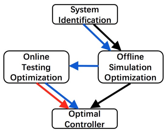
Figure 1.
Controller design procedures categorized by offline optimization (black), online optimization (red), and the proposed model-assisted online optimization method (blue).
In this paper, a highly nonlinear friction EGR valve system is modeled analytically with nonlinear friction, and the scheduled PID gains are tuned based on the proposed NSGA-II optimization algorithm using the offline optimized control gains as the initial setting. The closed-loop system performance is then validated through simulations and experimental studies. The main contribution of this paper is three-fold. First, an offline model-assisted scheduled PID gain tuning method based on the NSGA-II algorithm is proposed. Offline optimization through the simulation study provides a good initial ‘guess’ for online optimization. Second, the scheduled PID gains are optimized using the NSGA-II algorithm with reduced scheduling parameters based on the test bench input and output responses to make the online optimization feasible in terms of time and actuator durability constraints. Lastly, the coordinated offline–online optimization process is implemented in a microcontroller and the closed-loop system performance is validated by both simulations and experimental studies.
The rest of this paper is organized as follows. In Section 2, the detailed system model is depicted, experimentally validated, and used for offline optimization. Section 3 formulates the optimization problem of control gain tuning with defined control gain functions, objective functions, and decision-making criteria. Section 4 provides a step-by-step summary of the modified NSGA-II algorithm. In Section 5, the simulations and experimental setups are introduced and optimization results are presented along with associated discussions. Finally, Section 6 presents our conclusions and discusses future work.
2. Valve System Model
The nonlinear valve system architecture is shown in Figure 2, where the angular displacement , driven by a DC motor, is converted to the linear valve displacement y using a constrained slide rail–rod structure. Based on the valve structure in Figure 2, the relationship between and y can be expressed by (1):
where and y are the radian degree and valve opening percentage (%), respectively. The slide rod angular position is at the upright vertical position and the initial slide rod position is at rad (10 degrees), corresponding to the fully closed valve position (), meaning that when the valve is fully open (), the angle is rad (80 degrees); see the dashed-line in Figure 2.
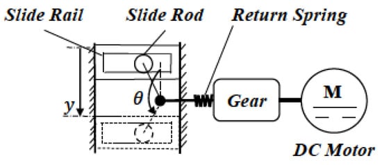
Figure 2.
Valve architecture.
The system moment of inertia J is calculated in (2), where is the total rotational assembly moment of inertia, is the equivalent moment of inertia of all the linear moving components at angular position , m is the total mass of linear moving part, and r is the length of the slide rod connection arm.
The valve dynamics can be described by (3) using Newton’s law.
where and represent the electric motor output torque and spring load torque, stated in (4) and (5), respectively; and are the motor torque and back EMF (electromagnetic fields) coefficients, respectively; , R, and represent the armature voltage, motor winding resistance, and spring preload position, respectively; is the nonlinear friction torque; and denotes the nonlinear torque created by the constraint of sliding rail–rod structure based on (6).
For the prominent nonlinear friction, the Stribeck friction model [34,35] is used, which calculates the friction force based on the relative speed between two contacted surfaces. Based on the Stribeck friction model, the friction torque can be represented by (7):
where , , and are the Coulomb friction torque, static friction torque, and viscous friction torque coefficients, respectively, and is the characteristic velocity.
To simplify the system identification process, the back EMF torque is lumped into the term in , resulting in motor torque , where u is the control input. Note that the scaled PWM (Pulse Width Modulation) range of u has been defined as based on the software interface used for system test bench, presenting the full duty cycle range of the H-bridge output in the control unit. With , the system dynamic equation is shown in (8).
Model coefficient identification is challenging in nonlinear systems. Multiple tests were conducted to isolate the effects of different parameters. First, the controller gain was obtained from valve specification data, then the spring stiffness , spring preload , and viscous friction were estimated by releasing the valve at different positions to generate the estimated Stribeck friction curve. Iterative calibrations were obtained by comparing the simulation and test responses to improve model accuracy. Based on the carefully calibrated model, two free falling cases (52.5% and 20.3% opening to 0%) were then compared using the experimental and model simulation results (Cases 1 and 2). In addition, the experimental closed-loop step response (0% opening to 50% opening, Case 3) using a PID controller (with gains P = 400, I = 0, and D = 0) was compared. The responses were closely matched (see Figure 3), validating the modeling accuracy. Detailed model parameters are shown in Table 1. The parameter units are omitted. as the system identification has been processed as “control input to system output”.
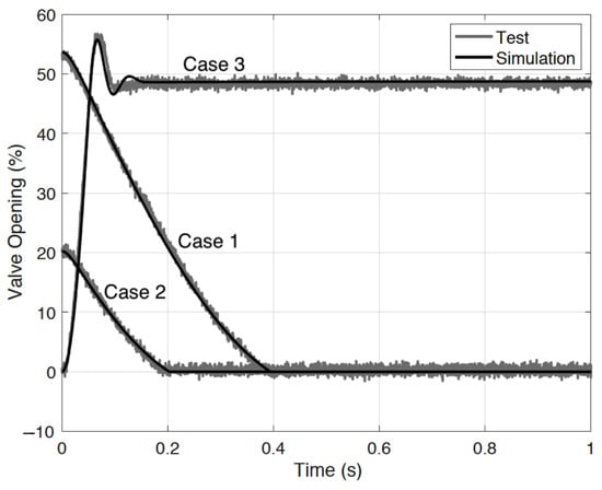
Figure 3.
Validation of the system model and its calibration.

Table 1.
Model parameters of EGR valve.
3. Problem Formulation
3.1. Gain-Scheduling Strategy
Based on the knowledge from bench tests and NSGA-II optimization of the fixed-gain PID controller (see the next section), the I (integration) and D (derivation) gains are relatively small compared with the P (proportion) gain. A large I gain results in quick windup, while a large D gain leads to high sensitivity to noise. Normally, the proportional, integral, and derivative scheduled gains (functions) should be optimized simultaneously, which increases the search space dimensions and results in an extremely high number of iterations needing to converge. In this paper, we aim to find an optimization scheme that is feasible for implementation; thus, we propose searching for the optimal scheduled PID gains sequentially in the three steps shown in Figure 4, where e denotes the valve position error between the reference and feedback signals.
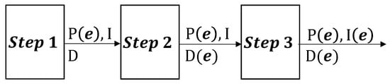
Figure 4.
Steps in sequential search for optimal gain-scheduled PID controller.
In Step 1, the algorithm searches for the optimal scheduling proportional gain function , along with the optimal fixed I and D gains; in Step 2, the scheduling derivative gain is optimized using the scheduling proportional gain obtained in Step 1 and the fixed I gain; finally, in Step 3, the scheduling integral gain is optimized using the proportional gain obtained from Step 1 and derivative gain obtained from Step 2.
Subject to the high static friction characteristics, the tracking error e of the valve position is selected as the scheduling parameter, where high gains are expected in the region with a small tracking error to overcome the increased friction force and reach the final destination. Considering the computational cost, the number of variables in the scheduled gain function should be low, even though complex scheduling functions could improve the closed-loop system performance further. After studying multiple candidate scheduling functions, is selected for the gain functions of P, I, and D for , where e is the position error and a, b, and c are the calibration parameters. Note that a saturation function is used here to avoid the gains going to infinity as goes to zero; see (9).
Figure 5 shows the scheduled-gain function with , , and b between 0.1 and 1. It can be seen that as b increases the scheduled gain magnitude increases significantly with a small position error, resulting in a large gain difference between small and large e compared to a relatively small b. With the help of the a (ramp-gain) and c (fixed-gain) parameters, the optimized scheduled gain is able to adapt to the nonlinear system dynamics.
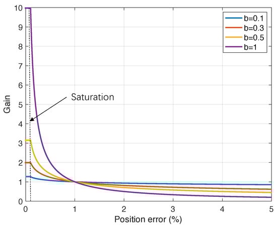
Figure 5.
Sample scheduled gains as a function of with a range of b.
The gain-scheduled PID controller structure is shown in Figure 6, where e and u represent the valve position error and control, respectively, while , , and are the scheduled proportional, integral, and derivative gains in the form of , respectively. In another words, the optimization aims to search for the best shape of , , and in the form of .
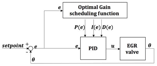
Figure 6.
Structure of gain-scheduled PID controller.
3.2. Objective Function
To obtain the optimal control performance under multiple operational conditions, four tests were designed to evaluate the proposed algorithm, as follows:
- 1.
- Case 1: Step response from close to 2% opening
- 2.
- Case 2: Step response from close to 50% opening
- 3.
- Case 3: Step response from close to 80% opening
- 4.
- Case 4: Step response from 50% to 30% opening
The ideal performance criteria are the closed-loop system settling time, overshoot, and steady-state error, which need to be included in the objective functions. Normally, in the single-objective optimization algorithm, the objective function can be defined as , i.e., the Integral of the Squared Error (ISE). However, for a system with high static friction, if the single objective function were used a large overshoot could exist in the optimized closed-loop response with minimal steady-state error. Thus, an additional objective function related to the percentage of overshoot (PO) is added to the objective function to form a multiple-objective optimization problem. Based on the preceding discussion, the two objective functions are defined below in (10):
where i represents the case number and the total number of cases is , while , , and s are the valve position, response peak, and settling time, respectively. Note that in this case the system percentage overshoot (PO) is associated with objective and both the settling time and steady-state error are considered in .
4. Non-Dominated Sorting Genetic Algorithm-II
In the traditional approach, multiple-objective optimization problems can be converted to single-objective optimization problems by predefining the weighting for each objective function. Thus, the optimal solution depends crucially on the selected weights. In addition, certain profitable trade-off relationships may be ignored, as a slight sacrifice of one objective function may lead to a significant improvement in the others. Using a different approach, the NSGA-II algorithm selects the optimal solutions on a Pareto front, which includes multiple non-dominated solutions. The trade-off relationship between each objective can be clearly presented, allowing the decision-maker to pick the optimal solutions based on specific criteria. Note that there is no unique way to select the optimal individual solution among the nondominated solution set from NSGA-II, as the performance evaluation criteria vary with different requirements. In this work, reference point-based multiple-criteria decision-making (MCDM) [36] is applied by considering the origin point as the reference point, with equal weights for objectives and . Thus, the point on the Pareto front with minimum distance to the origin () is selected as the ultimate solution.
The detailed NSGA-II optimization method implemented in this paper is described below, along with the parameters predefined for calibrating the PID scheduled gains; see [28,33] for details.
- 1.
- Initialization: Letting , the initial parent population is generated with size . For each individual, all decision variables are randomly generated among the related search space with .
- 2.
- Nondomination sorting: The resulting individual is evaluated based on the nondomination level with the nondomination rank (rank 1 is the best level, rank 2 is the next-best level, etc.) assigned.
- 3.
- Offspring generation: The usual binary tournament selection is applied, with binary crossover at probability and distribution index, polynomial mutation at probability, and distribution index for generating an offspring population with size equal to .
- 4.
- Combination and sorting: An extended set is generated by combining and with a size of . After nondominated sorting (as stated in Step 2), selection starts from low ranked individuals and continues to form a new population of size until it is filled. If the rank of multiple individuals is the same and the remaining space in is limited, individuals with larger crowding distance have priority in selection; for further details on crowding distance, see [28]. Lastly, the new population set is filled with the selected individuals.
- 5.
- Iteration: After updating the generation , Steps 2 to 4 are repeated until the stopping criterion is satisfied.
To demonstrate the advantages of the gain-scheduled PID controller, a fixed-gain PID controller was optimized for the high static friction model using NSGA-II. To ensure a fair comparison, an identical search space, population, and generation size to the gain-scheduled case were selected.
5. Iterative NSGA-II
The structure of the iterative NSGA-II algorithm is shown in Figure 7. The initial search space is defined as the region centered on the initial solution obtained from the offline simulation. Within a small search area, NSGA-II can find the regional optimal Pareto front quickly with a small population size in only a few generations. However, when looking into the distribution of the decision variables, there may be variables that are saturated over the Pareto front on the boundary of the search space. This indicates that the objective function costs can be further improved if the search space can be shifted towards the boundary direction (second search space); see the blue arrow shown in Figure 7. Following the NSGA-II search over the second search space, the solved Pareto front from the first and second search spaces is combined and sorted to generate a new Pareto front. Distribution evaluation is applied again to determine whether or not another search space shift is necessary. The search is stopped when the distribution indicates that the optimal solution has been found or the pre-defined maximum shift limit has been reached. As a result, this iterative NSGA-II method can improve optimization performance with a relatively small search space, making it feasible for real-time implementation. During online bench optimization, the decision variables (PID control gains) are saturated by predefining the search space in each iteration of NSGA-II optimization; the details are stated in Section 7.
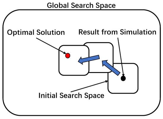
Figure 7.
Iterative NSGA-II procedure; the search space starts with offline simulation and evolves within the global search space to arrive at the optimal solution.
6. Offline Optimization
In this section, the optimization structure is discussed, then the step response performance of the solved gain-scheduled PID controller is compared with the fixed-gain one. Finally, additional disturbance tests are applied to investigate the possibility of further improving the gain-scheduled PID controller.
6.1. Optimization Structure
To generate the baseline simulation, MATLAB R2019b software created by MathWorks was used in East Lansing, US (see Figure A1 in Appendix A for the MATLAB Simulink model) for the iterative NSGA-II search. The data were connected through the MATLAB workspace, as both MATLAB and Simulink can read and write data in the MATLAB workspace. The detailed optimal gain-scheduled PID controller search structure using NSGA-II is described in Figure 8, where, as implemented in MATLAB, NSGA-II generates a next generation for each iteration and updates it to the workspace. In addition, the MATLAB–Simulink environment described above was used to evaluate the whole generation and feed the performance results back to MATLAB to obtain the next generation.
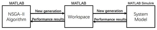
Figure 8.
Simulation structure used for iterative search.
6.2. Offline Optimized Proportional Gain-Scheduled PID Controller
First, let the scheduled gain be with fixed I and D gains and obtain the Pareto front of the two objectives ( and ) using the NSGA-II algorithm using the parameters summarized in Table 2, where is defined in (9).
Table 2.
Genetic Algorithm parameters used in Step 1.
Figure 9 shows the non-dominated solutions of both the gain-scheduled and fixed-gain PID controllers after 100 generations. Note that the Pareto front of the gain-scheduled PID controller is much closer to the origin, indicating improved closed-loop performance over the fixed-gain controller. The optimal averaged step response overshoot is restricted to 0.01% and 0.04% for scheduled and fixed-gain PID controllers, respectively, and the optimal ISEs are 4.68% and 4.79%. In addition, the widely distributed results from the gain-scheduled PID controller indicate that it provides more multifarious controller options for decision-makers based on different system performance requirements. For example, if a fast settling time with a minimal steady-state error is much more crucial than minimizing the overshoot, the solution at the lower right corner of the Pareto front can be selected to satisfy these requirements.
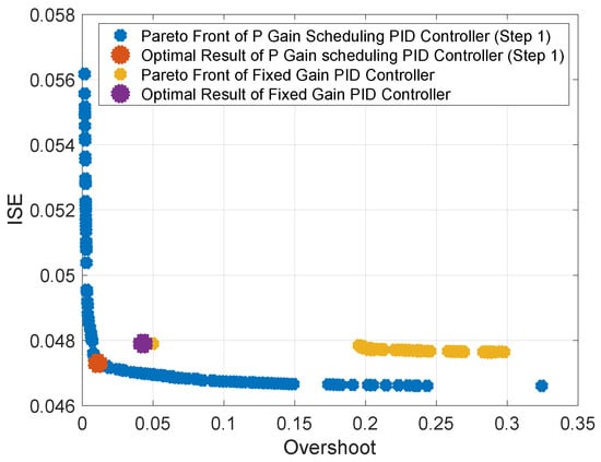
Figure 9.
Pareto fronts of scheduled P and fixed P gain controllers.
Optimization solutions for both the scheduled and fixed P gain PID controllers, with I and D gains fixed in both cases, are summarized in Table 3, with both controllers selected based on the multiple-criteria decision-making method. In this case, considering equivalent significance of both the system overshoot and ISE , the point with minimal distance to the origin is selected as the optimal result. With the scheduled P gain PID controller, the objective functions (overshoot) and (ISE) are minimized to and , compared with and for the fixed-gain case, representing an improvement of 74% and 1.3%, respectively.
Table 3.
Optimal controller parameters for Step 1.
6.3. Offline Optimized PID Gain-Scheduled Controller
In Step 2, based on the proportional gain function from Step 1, the initial scheduled derivative gain function D is selected as and optimized following the same process as Step 1 to obtain coefficients a, b, and c, with the scheduled gain P from Step 1 and the integral gain I fixed. The optimization parameters are shown in Table 4.
Table 4.
Genetic Algorithm parameters used in Step 2.
In Step 3, the initial scheduled integral gain I is in the form , and is optimized in Step 3 using the gain-scheduled P and I from Steps 1 and 2, respectively. The optimization parameters are shown in Table 5.
Table 5.
Genetic Algorithm parameters used in Step 3.
The solution of the optimal gain-scheduled PID controller is shown in Equation (11), with the associated evolution of Pareto front for each step shown in Figure 10. Note that part of the Pareto front in Step 1 is outside the plot.
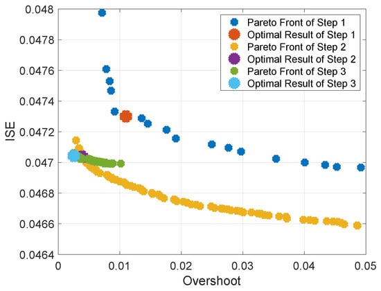
Figure 10.
Pareto fronts of the gain-scheduled PID controller.
With the scheduled optimal derivative gain obtained in Step 2, both objective functions (overshoot) and (ISE) have been improved to from 0.0110 and 0.0473 to 0.0039 and 0.0470, representing an improvement of 64.5% and 0.6%, respectively. Finally, after Step 3, and are optimized to 0.0025 and 0.0470, a 35.9% and 0% improvement, respectively, over Step 2. To investigate the optimality, the scheduled function of the proportional gain P is re-optimized using the scheduled D and I gains from Steps 2 and 3, with the optimized result showing only a negligible improvement. Because the offline optimized (initial) gain-scheduled PID controller is intended to be further optimized online, the optimization results from Step 3 are sufficient.
The step responses of the initial optimal controller are shown in Figure 11, with the associated performance improvements summarized in Table 6; the case numbers refer to these described in Section 3.2, while the notations G-S and F-G denote the gain-scheduled (G-S) and fixed-gain (F-G) PID controllers, respectively.
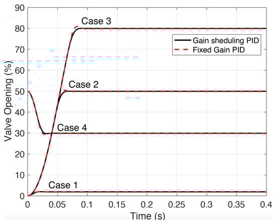
Figure 11.
Step responses of optimized initial controller.
Table 6.
Offline optimized controller performance summary.
Compared with the fixed-gain PID controller, the (Overshoot) and (ISE) are optimized to 0.0025 and 0.0470, which represents an improvement of 94.2% and 1.9%, respectively. In the detailed cases, regarding the steady-state error, both controllers handle it well in Cases 2, 3, and 4, with all of them being below 1%. Note that for an EGR valve it is desirable to have no overshoot; however, for the small opening case (Case 1), the fixed-gain PID controller has an 8.2% overshoot, compared with 3.8% for the optimal initial gain-scheduled PID controller. In order to find the root cause of this result, a detailed comparison is shown in Figure 12.
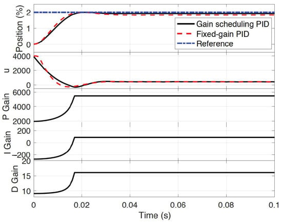
Figure 12.
Step responses with 2% valve opening.
The control inputs of both the gain-scheduled and fixed-gain controllers are shown in the middle plot of Figure 12, with their associated responses shown in the upper plot. With a large fixed proportional gain, the fixed-gain PID controller provides a fast response at the beginning; however, when the valve closes to its setpoint, the response slows down more quickly than that of the gain-scheduled controller, leading to a larger steady-state error for the fixed-gain controller. Note that the gain-scheduled controller increases the control gain significantly within the small error region to fight the static friction. Based on the control effort, although the fixed-gain PID controller has a fairly large P gain, it is not large enough to overcome the static friction when the valve is closed to its setpoint. On the other hand, the gain-scheduled PID controller increases the proportional gain significantly when the valve is close to its setpoint in order to overcome the large static friction; see the bottom plot in Figure 12.
7. Online Optimization and Experimental Validation
7.1. Test Bench Setup
The proposed online optimization bench setup is shown in Figure 13. An Arduino MKR 1000 board was used as the real-time controller along with an MKR 1000 Motor Carrier board for driving the DC motor on the EGR valve. Note that the MKR board is mainly used to sample the position sensor signal and output the motor control signal to the Motor Drive board. The host computer for the control strategy calculations used an Intel Core i5-7200 CPU. The NSGA-II algorithm was implemented into MATLAB using the same structure as the offline simulation one depicted Figure 8, with the right side of the Matlab/Simulink model in Figure 8 replaced by real-world hardware, including the EGR valve and Arduino MKR 1000 Motor Carrier board. The Arduino board is programmable through the MATLAB–Simulink interface, which allowed us to process new generation variables and test results between the host computer and test bench. The Arduino MKR 1000 board was used as the real-time controller along with the MKR 1000 Motor Carrier board for driving the DC motor on the EGR valve; see “Control and Drive Board” in Figure 13. For each generation, all the population members carrying the control parameter set were compiled within the controller in sequence, with the position feedback signal sampled from the valve position sensor to the board and saved in the host computer for the next iteration. Unlike the simulation study, during each bench test the NSGA-II program in MATLAB did not wait for the bench test to finish and send the result back for evaluation. Thus, a pause was added in the NSGA-II program after the scheduled gains were compiled in the controller, allowing the performance test to be completed before starting the next evaluation.
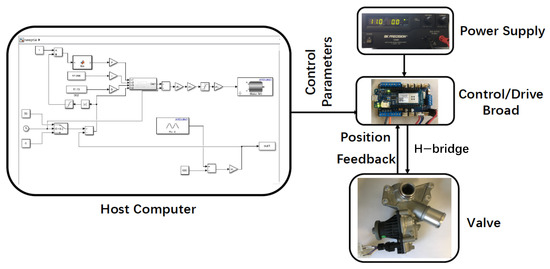
Figure 13.
Online NSGA-II optimization test bench setup.
7.2. Problem Formulation of EGR Valve PID Controller Tuning
In the offline model-based optimization, the optimal gain-scheduled function is solved by searching the three variables defined in (9). For the online optimization, the original problem formulation stated in Section 3 is too complex to use, as it could lead to large population sizes and a large number of generations due to the larger number of decision variables. In addition, the shape variation of the gain-scheduled function could bring additional complexity in the NSGA-II iterative strategy due to physical system noise and nonlinearity. As a result, the optimization problem is simplified with the structure shown in Figure 14, where * denotes the multiplication sign, , , and are the solved optimal initial gain-scheduled functions from the offline optimization, e and u are the position error and control output, respectively, and the scaling parameters , , and represent the decision variables used for the online NSGA-II search associated with the , , and terms. In other words, the shape of the gain-scheduled function is fixed during the online optimization using only changes in magnitude.
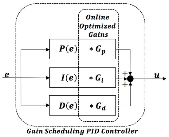
Figure 14.
Decision variables for online NSGA-II optimization bench test.
7.3. Online Optimization
First, the step responses of the simulation and experimental studies are shown in Figure 15; it can be seen that the initial and intermediate responses of the experimental result closely match the simulated ones, as the system model is relatively accurate. However, the simulated and experimental responses deviate when the valve approaches the setpoint. Although a well-calibrated Stribeck friction curve can be used to describe the nonlinearity of friction at low valve velocity, a modeling error remains, leading to the degradation of control performance. Therefore, it was necessary to conduct an online optimization study based on the offline optimized controller to further improve the closed-loop system performance. By analyzing the offline simulation results, it was found that as long as the optimal scheduled gain function is obtained, the optimal gain-scheduled PID controller can be used under different operational conditions. Therefore, to reduce computational cost and the required number of experiments, the 0 to 50 percent opening case was selected for online optimization.
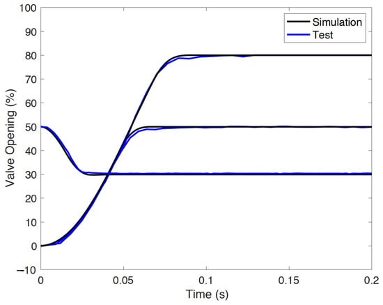
Figure 15.
Step responses using offline optimized controller.
Using the binary crossover probability and distribution index at and with the polynomial mutation probability and distribution index at and from the simulation study, the parameters for the online optimization study are listed in Table 7. Benefiting from the iterative search structure, the initial search space of , , and can be defined in a relatively small range ( here). By evaluating the results of the first search, certain saturations can be observed for , , and near the Pareto front, which leads to search space migration in the second iteration. As can be seen from Figure 16, after migrating the search space, the overall performance of both the whole population and Pareto-front population in the second iteration (the orange dots) are improved over the first iteration (the blue dots). Finally, the yellow circled point is selected as the optimal solution, as it has a minimal distance to the origin and results in improved online optimization of the control performance (see Figure 17). In summary, a comparison of the offline fixed gain (F-G), offline gain scheduling (G-S), and online optimized (O-G-S) PID controller is shown in Table 8.
Table 7.
Details of online optimization using iterative NSGA-II.
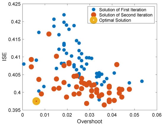
Figure 16.
Result points of online NSGA-II optimization.
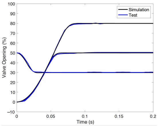
Figure 17.
Step responses of offline–online co–optimized controller.
Table 8.
Summary of controller performance with 50% valve opening step response.
8. Conclusions and Future Work
In this paper, we have presented an offline model-assisted online optimization method to automatically tune the gain-scheduled PID gains for an exhaust gas recirculation (EGR) valve with large nonlinear friction. The optimized gain-scheduled PID controller can adaptively compensate for the increased friction force in low-velocity regions. In the optimization problem, two objective functions are proposed to consider commonly used performance indices such as the settling time, overshoot, and steady-state error. The NSGA-II optimization results can provide decision-makers with a Pareto front that clearly shows the trade-offs. The optimal initial gain-scheduled functions are obtained using the multi-objective NSGA-II algorithm, eliminating the process of manually tuning control gains. Next, the proposed online iterative NSGA-II optimization approach is used to further optimize the closed-loop system performance, significantly reducing the need for bench tests. Our experimental results show that the proposed automatically tuned optimal gain-scheduled PID controller has better overall performance than a fixed-gain controller.
In future work, the proposed algorithm based on offline and online co-optimization can be extended to optimize advanced controllers, such as model predictive control and learning-based control. Although this paper provides a meaningful attempt to combine prior model knowledge with black-box online learning, it is interesting and worthwhile to develop analytical tools to study the resulting system’s robustness and optimality. Earlier work on model-based control can provide useful insights in this direction [37]. Of particular interest, constraints on states and control inputs as well as learning-based control can be further included in the proposed algorithm to enable computationally efficient tuning of online-learning control. In addition, comparison studies with other data-driven PID automatic tuning algorithms, such as the Monte Carlo method, are meaningful and will be part of our future work.
Author Contributions
Conceptualization, S.Q. and G.Z.; methodology, S.Q. and G.Z.; software, S.Q.; validation, S.Q. and G.Z.; formal analysis, S.Q., T.H. and G.Z.; investigation, S.Q.; resources, S.Q.; data curation, S.Q.; writing—original draft preparation, S.Q.; writing—review and editing, T.H. and G.Z.; visualization, S.Q.; supervision, G.Z. and T.H.; project administration, G.Z. All authors have read and agreed to the published version of the manuscript.
Funding
This research received no external funding.
Conflicts of Interest
The funders had no role in the design of the study; in the collection, analyses, or interpretation of data; in the writing of the manuscript, or in the decision to publish the results.
Appendix A. Simulink Model
See Figure A1 for the Simulink offline NSGA-II model.

Figure A1.
MATLAB−Simulink Program used for offline NSGA-II optimization.
References
- Xie, W.F. Sliding-mode-observer-based adaptive control for servo actuator with friction. IEEE Trans. Ind. Electron. 2007, 54, 1517–1527. [Google Scholar] [CrossRef]
- Shen, Q.; Tianyi, H.; Guoming, G.Z. Switched LPV Modeling and Control of an Engine EGR Valve with Dry Friction. In Proceedings of the 2019 IEEE Conference on Control Technology and Applications (CCTA), Hong Kong, China, 19–21 August 2019. [Google Scholar]
- Qu, S.; Zhu, G.; Su, W.; Shan-Min Swei, S. Linear parameter-varying-based transition flight control design for a tilt-rotor aircraft. Proc. Inst. Mech. Eng. Part G J. Aerosp. Eng. 2022, 236, 3354–3369. [Google Scholar] [CrossRef]
- Qu, S.; Zhu, G.; Su, W.; Swei, S.S.M. LPV Model-based Adaptive MPC of an eVTOL Aircraft During Tilt Transition Subject to Motor Failure. Int. J. Control. Autom. Syst. 2023, 21, 339–349. [Google Scholar] [CrossRef]
- Qu, S.; He, T.; Zhu, G.G. Engine EGR valve modeling and switched LPV control considering nonlinear dry friction. IEEE/ASME Trans. Mechatron. 2020, 25, 1668–1678. [Google Scholar] [CrossRef]
- Qu, S.; Zhu, G.; Su, W.; Shan-Min Swei, S.; Hashimoto, M.; Zeng, T. Adaptive model predictive control of a six-rotor electric vertical take-off and landing urban air mobility aircraft subject to motor failure during hovering. Proc. Inst. Mech. Eng. Part G J. Aerosp. Eng. 2022, 236, 1396–1407. [Google Scholar] [CrossRef]
- Zhao, Z.Y.; Tomizuka, M.; Isaka, S. Fuzzy gain scheduling of PID controllers. IEEE Trans. Syst. Man, Cybern. 1993, 23, 1392–1398. [Google Scholar] [CrossRef]
- Blanchett, T.; Kember, G.; Dubay, R. PID gain scheduling using fuzzy logic. ISA Trans. 2000, 39, 317–325. [Google Scholar] [CrossRef]
- Åström, K.J.; Hägglund, T.; Astrom, K.J. Advanced PID Control; ISA-The Instrumentation, Systems, and Automation Society Research Triangle; International Society of Automation: Pittsburgh, PA, USA, 2006; Volume 461. [Google Scholar]
- Ogata, K. Moden Control Engineering; Prentice Hall: Hoboken, NJ, USA, 2010. [Google Scholar]
- Liu, G.; Daley, S. Optimal-tuning nonlinear PID control of hydraulic systems. Control. Eng. Pract. 2000, 8, 1045–1053. [Google Scholar] [CrossRef]
- Korkmaz, M.; Aydoğdu, Ö.; Doğan, H. Design and performance comparison of variable parameter nonlinear PID controller and genetic algorithm based PID controller. In Proceedings of the 2012 International Symposium on Innovations in Intelligent Systems and Applications, Trabzon, Turkey, 2–4 July 2012; pp. 1–5. [Google Scholar]
- Valluru, S.K.; Singh, M. Performance investigations of APSO tuned linear and nonlinear PID controllers for a nonlinear dynamical system. J. Electr. Syst. Inf. Technol. 2018, 5, 442–452. [Google Scholar] [CrossRef]
- Isayed, B.M.; Hawwa, M.A. A nonlinear PID control scheme for hard disk drive servosystems. In Proceedings of the 2007 Mediterranean Conference on Control & Automation, Athens, Greece, 27–29 June 2007; pp. 1–6. [Google Scholar]
- Su, Y.; Sun, D.; Duan, B. Design of an enhanced nonlinear PID controller. Mechatronics 2005, 15, 1005–1024. [Google Scholar] [CrossRef]
- Zaidner, G.; Korotkin, S.; Shteimberg, E.; Ellenbogen, A.; Arad, M.; Cohen, Y. Non Linear PID and its application in Process Control. In Proceedings of the 2010 IEEE 26-th Convention of Electrical and Electronics Engineers in Israel, Eilat, Israel, 17–20 November 2010; pp. 574–577. [Google Scholar]
- Gharghory, S.; Kamal, H. Modified PSO for optimal tuning of fuzzy PID controller. Int. J. Comput. Sci. Issues (IJCSI) 2013, 10, 462. [Google Scholar]
- Tang, K.S.; Man, K.F.; Chen, G.; Kwong, S. An optimal fuzzy PID controller. IEEE Trans. Ind. Electron. 2001, 48, 757–765. [Google Scholar] [CrossRef]
- Li, H.X.; Zhang, L.; Cai, K.Y.; Chen, G. An improved robust fuzzy-PID controller with optimal fuzzy reasoning. IEEE Trans. Syst. Man Cybern. Part B 2005, 35, 1283–1294. [Google Scholar] [CrossRef]
- Jantzen, J. Tuning of Fuzzy PID Controllers; Technical University of Denmark, Department of Automation: Lyngby, Denmark, 1998; Volume 326. [Google Scholar]
- Visioli, A. Tuning of PID controllers with fuzzy logic. IEEE Proc.-Control Theory Appl. 2001, 148, 1–8. [Google Scholar] [CrossRef]
- Koza, J.R. Genetic Programming 1997: Proceedings of the Second Annual Conference, Stanford, CA, USA, 13–16 July 1997; Morgan Kaufmann Publishers: Burlington, MA, USA, 1997. [Google Scholar]
- Whitley, D. A genetic algorithm tutorial. Stat. Comput. 1994, 4, 65–85. [Google Scholar] [CrossRef]
- Pereira, D.S.; Pinto, J.O. Genetic algorithm based system identification and PID tuning for optimum adaptive control. In Proceedings of the 2005 IEEE/ASME International Conference on Advanced Intelligent Mechatronics, Monterey, CA, USA, 24–28 July 2005; pp. 801–806. [Google Scholar]
- Mitsukura, Y.; Yamamoto, T.; Kaneda, M. A design of self-tuning PID controllers using a genetic algorithm. In Proceedings of the 1999 American Control Conference (Cat. No. 99CH36251), San Diego, CA, USA, 2–4 June 1999; Volume 2, pp. 1361–1365. [Google Scholar]
- Saad, M.S.; Jamaluddin, H.; Darus, I.Z. PID controller tuning using evolutionary algorithms. Wseas Trans. Syst. Control 2012, 7, 139–149. [Google Scholar]
- Murata, T.; Ishibuchi, H. MOGA: Multi-objective genetic algorithms. In Proceedings of the IEEE International Conference on Evolutionary Computation, Perth, WA, Australia, 29 November–1 December 1995; Volume 1, pp. 289–294. [Google Scholar]
- Deb, K.; Pratap, A.; Agarwal, S.; Meyarivan, T. A fast and elitist multiobjective genetic algorithm: NSGA-II. IEEE Trans. Evol. Comput. 2002, 6, 182–197. [Google Scholar] [CrossRef]
- Ayala, H.V.H.; dos Santos Coelho, L. Tuning of PID controller based on a multiobjective genetic algorithm applied to a robotic manipulator. Expert Syst. Appl. 2012, 39, 8968–8974. [Google Scholar] [CrossRef]
- Panda, S. Multi-objective PID controller tuning for a FACTS-based damping stabilizer using non-dominated sorting genetic algorithm-II. Int. J. Electr. Power Energy Syst. 2011, 33, 1296–1308. [Google Scholar] [CrossRef]
- Pedersen, G.K.; Yang, Z. Multi-objective PID-controller tuning for a magnetic levitation system using NSGA-II. In Proceedings of the 8th Annual Conference on Genetic and Evolutionary Computation, Seattle, WA, USA, 8–12 July 2006; pp. 1737–1744. [Google Scholar]
- Guan, X.Z. Multi-objective PID controller based on NSGA-II algorithm with application to main steam temperature control. In Proceedings of the 2009 International Conference on Artificial Intelligence and Computational Intelligence, Shanghai, China, 7–8 November 2009; Volume 4, pp. 21–25. [Google Scholar]
- Pal, A.; Zhu, L.; Wang, Y.; Zhu, G. Data-driven model-based calibration for optimizing electrically boosted diesel engine performance. Int. J. Engine Res. 2022, 24, 1515–1529. [Google Scholar] [CrossRef]
- Olsson, H.; Åström, K.J.; De Wit, C.C.; Gäfvert, M.; Lischinsky, P. Friction models and friction compensation. Eur. J. Control 1998, 4, 176–195. [Google Scholar] [CrossRef]
- Andersson, S.; Söderberg, A.; Björklund, S. Friction models for sliding dry, boundary and mixed lubricated contacts. Tribol. Int. 2007, 40, 580–587. [Google Scholar] [CrossRef]
- Wierzbicki, A.P. Reference point approaches and objective ranking. In Practical Approaches to Multi-Objective Optimization; Dagstuhl Seminar Proceedings; Schloss Dagstuhl-Leibniz-Zentrum für Informatik: Dagstuhl, Germany, 2007. [Google Scholar]
- He, T.; Chen, X.; Zhu, G.G. A Dual-Loop Robust Control Scheme With Performance Separation: Theory and Experimental Validation. IEEE Trans. Ind. Electron. 2022, 69, 13483–13493. [Google Scholar] [CrossRef]
Disclaimer/Publisher’s Note: The statements, opinions and data contained in all publications are solely those of the individual author(s) and contributor(s) and not of MDPI and/or the editor(s). MDPI and/or the editor(s) disclaim responsibility for any injury to people or property resulting from any ideas, methods, instructions or products referred to in the content. |
© 2023 by the authors. Licensee MDPI, Basel, Switzerland. This article is an open access article distributed under the terms and conditions of the Creative Commons Attribution (CC BY) license (https://creativecommons.org/licenses/by/4.0/).