Article

Distributed GNE Seeking under Global-Decision and Partial-Decision Information over Douglas-Rachford Splitting Method

Chongqing Key Laboratory of Nonlinear Circuits and Intelligent Information Processing, College of Electronic and Information Engineering, Southwest University, Chongqing 400715, China
*
Author to whom correspondence should be addressed.
Appl. Sci. 2023, 13(12), 7058; https://doi.org/10.3390/app13127058
Submission received: 12 April 2023 / Revised: 24 May 2023 / Accepted: 9 June 2023 / Published: 12 June 2023
(This article belongs to the Special Issue Advanced Artificial Intelligence Theories and Applications)

Abstract

:
This paper develops an algorithm for solving the generalized Nash equilibrium problem (GNEP) in non-cooperative games. The problem involves a set of players, each with a cost function that depends on their own decision as well as the decisions of other players. The goal is to find a decision vector that minimizes the cost for each player. Unlike most of the existing algorithms for GNEP, which require full information exchange among all players, this paper considers a more realistic scenario where players can only communicate with a subset of players through a connectivity graph. The proposed algorithm enables each player to estimate the decisions of other players and update their own and others’ estimates through local communication with their neighbors. By introducing a network Lagrangian function and applying the Douglas-Rachford splitting method (DR), the GNEP is reformulated as a zero-finding problem. It is shown that the DR method can find the generalized Nash equilibrium (GNE) of the original problem under some mild conditions.

1. Introduction

In recent years, the generalized Nash equilibrium (GNE) [1,2], has been increasingly applied to solve practical problems. Examples include electricity market scheduling [3], peer-to-peer electricity market analysis [4] and energy trading in combined heat and power market [5]. In a noncooperative game, there are both shared and unshared constraints. These constraints cause players’ private costs and feasible decision sets to interact with each other. In such a situation, it is necessary to establish rules for the players. The players make decisions by exchanging information according to the rules. A Nash equilibrium can be found as long as the rules are appropriate.
Algorithms for solving Nash equilibrium problems can be classified as centralized optimization algorithms and distributed optimization algorithms based on the way they solve optimization problems. In a centralized optimization algorithm, the entire problem is solved by a single entity with access to all the necessary information. In contrast, distributed optimization algorithms solve the problem by decomposing it into smaller sub-problems that are cooperatively solved by multiple players. This paper mainly studies distributed optimization algorithms. The information setting of distributed optimization algorithms is also divided into two types. The first type requires each player to publicly disclose their decision information. Another type only requires players to disclose information to their neighbors. In this paper, these rules are referred to as “global information setting” and “partial information setting”, respectively.
Since the 1950s, research on GNEP has gradually become a hot topic [6,7,8,9]. For the solving of Nash equilibrium problems, many distributed algorithms have been studied in recent years, such as an algorithm based on the forward-backward operator partitioning method [10], a triangular preconditioned proto-dual algorithm [11] and an algorithm fully adapted to monotone variational inequalities [12]. In [13], Lacra Pavela proposes a distributed primal-dual algorithm for the computation of generalized Nash equilibria (GNE) in noncooperative games in networked systems. The algorithm handles games with shared affine coupling constraints via operator splitting methods. In contrast, the Algorithm 1 proposed in this paper has a higher convergence speed. [14] reformulates the GNE problem as a variational inequality problem and solves it through the doubly augmented operator splitting method (DAOS). This method can handle nonsmooth and nonconvex objective functions and constraints. In contrast, the Algorithm 1 proposed in this paper solves the optimization problem by using unconstrained optimization and linear mapping, which has higher computational efficiency. Moreover, some studies have combined the ideas of machine learning to solve optimization problems. By combining extremum-seeking control (ESC) with learning algorithms, Feng Xiao, Xin Cai and Bo Wei proposed a GNE-seeking algorithm in [15]. This algorithm can be executed in a partial information setting and does not require knowledge of the explicit expression of the cost function. In most of the current research, only algorithms under the local information setting are studied. This paper discusses two forms of algorithms under two information settings. It also shows intuitively through experiments that the algorithm under the local information setting has higher efficiency.
Algorithm 1 GNE seeking under partial-decision
  • Initialize: For each player i N , let x i , 0 [ i ] R n i , x i , 0 [ i ] R n n i , z i , 0 R m and λ i , 0 R m .
  •    for  k = 1 , 2 ,  do
  •      x ˘ i , k [ i ] = x i , k [ i ] + 1 2 c α i j = 1 N w i j ( x i , k [ j ] x i , k [ i ] )
  •      x ˘ i , k = p r o x α i f i { x i , k + 1 2 c α i j = 1 N w i j ( x i , k [ j ] x i , k ) 1 2 α i A i T λ i , k ) }
  •      z ˘ i , k = z i , k + 1 2 τ i j = 1 N w i j ( λ j , k λ i , k )
  •      λ ˘ i , k = λ i , k 1 2 γ i A i x i , k 1 2 γ i j = 1 N w i j ( z i , k z j , k ) γ i b + γ i A i x ˘ i , k γ i j = 1 N w i j ( z ˘ j , k z ˘ i , k )
  •      x ˜ i , k = 2 x ˘ i , k x i , k
  •      x ˜ i , k [ i ] = 2 x ˘ i , k [ i ] x i , k [ i ]
  •      z ˜ i , k = 2 z ˘ i , k z i , k
  •      λ ˜ i , k = 2 λ ˘ i , k λ i , k
  •      x ¯ i , k [ i ] = x ˜ i , k [ i ] + 1 2 c α i j = 1 N w i j ( x ˜ i , k [ j ] x ˜ i , k [ i ] )
  •      x ¯ i , k = p r o x α i f i { x i , k + 1 2 c α i j = 1 N w i j ( x ˜ i , k [ j ] x ˜ i , k ) 1 2 α i A i T λ ˜ i , k }
  •      z ¯ i , k = z ˜ i , k + 1 2 τ i j = 1 N w i j ( λ ˜ j , k λ ˜ i , k )
  •      λ ¯ i , k = λ i , k 1 2 γ i A i x ˜ i , k 1 2 γ i j = 1 N w i j ( z ˜ i , k z ˜ j , k ) γ i b + γ i A i x ¯ i , k + γ i j = 1 N w i j ( z ¯ i , k z ¯ j , k )
  •      x i , k + 1 = x i , k + 2 r k x ¯ i , k 2 r k x ˘ i , k
  •      x i , k + 1 [ i ] = x i , k + 2 r k x ¯ i , k [ i ] 2 r k x ˘ i , k [ i ]
  •      z i , k + 1 = z i , k + 2 r k z ¯ i , k 2 r k z ˘ i , k
  •      λ i , k + 1 = λ i , k + 2 r k λ ¯ i , k 2 r k λ ˘ i , k
  •    end for
  • Retuen: The sequence ( x i , k [ i ] , x i , k [ i ] ) k = 1 will eventually approximate the optimal solution.
The Douglas-Rachford splitting method used in this paper can handle nonsmooth convex functions and even non-convex functions, in addition to being able to use random block coordinate strategies and asynchronous execution to improve efficiency and robustness. This approach has been widely used to study graph coloring [16], compression perception [17], and image denoising [18].
The contributions of this paper can be summarized as follows:
  • Two new variants of the Douglas-Rachford algorithm are proposed in this paper, denoted as Algorithms 1 and 2, which can solve Nash equilibrium problems.
  • Two pairs of new splitting operators are introduced for Algorithms 1 and 2, respectively, which can ensure the convergence and efficiency of the algorithms.
  • Algorithm 2 is proved in this paper, and it has a linear convergence rate under the global information setting, while Algorithm 1 has a faster convergence rate under the local information setting.
  • The theoretical results in this paper are verified by numerical experiments and the advantages of Algorithm 1 are shown by comparison with the existing method.
Algorithm 2 GNE seeking under global-decision
  • Initialize: For each player i N , let x i , 0 R n i , z i , 0 R m and λ i , 0 R m
  •    for  k = 1 , 2 , 3 ,  do
  •      x ˘ i , k = arg min x ( 1 2 x ( x i , k α i A i T λ i , k ) 2 + α i f i ( x i , x i ) )
  •      z ˘ i , k = τ i j = 1 N w i j ( λ j , k λ i , k ) + z ˘ i , k
  •      λ ˘ i , k = λ i , k 1 2 γ i A i x i , k 1 2 γ i j = 1 N w i j ( z i , k z j , k ) γ i b i + γ i A i x ˘ i , k + γ i j = 1 N w i j ( z ˘ i , k z ˘ j , k )
  •      x ˜ i , k = 2 x ˘ i , k x i , k
  •      z ˜ i , k = 2 z ˘ i , k z i , k
  •      λ ˜ i , k = 2 λ ˘ i , k λ i , k
  •      x ¯ i , k = p r o x a i g i { x ˜ i , k 1 2 α i A i T λ ˜ i , k }
  •      z ¯ i , k = 1 2 γ i j = 1 N w i j ( λ ˜ j , k λ ˜ i , k ) + z ˜ i , k
  •      λ ¯ i , k = p r o j R 0 m ( λ ˜ i , k 1 2 γ i A i x ˜ i , k 1 2 γ i j = 1 N w i j ( z ˜ i , k z ˜ j , k ) + γ i A i x ¯ i , k + γ i j = 1 N w i j ( z ¯ i , k z ¯ j , k ) )
  •      x i , k + 1 = x i , k + 2 r k x ¯ i , k 2 r k x ˜ i , k
  •      z i , k + 1 = z i , k + 2 r k z ¯ i , k 2 r k z ˜ i , k
  •      λ i , k + 1 = λ i , k + 2 r k λ ¯ i , k 2 r k λ ˜ i , k
  •    end for
  • Retuen: The sequence ( x i , k ) k = 1 will eventually approximate the optimal solution.
In this paper, Section 2 derives the KKT conditions of the variational problem of the original game using dual analysis method; Section 3 proposes distributed Algorithms 1 and 2 based on DR; Section 4 analyzes the convergence of the two algorithms; Section 5 presents the simulation results of these two algorithms; and Section 6 summarizes the whole paper and looks forward to the future.

2. Preliminary Acquaintance

2.1. Graph Theory

The graph G is mainly represented by two sets, namely the set of vertices N and the set of edges ε , i.e., G = { N , ε } , where N = { 1 , , N } and ε N × N . A player i and a player j are said to be neighbors of i if they can exchange information, and this relationship is represented in the connectivity graph as ( i , j ) ε . Moreover, the set of neighbors of player i is N i = { j | ( i , j ) ε } . A path in a graph G is an interleaved sequence of vertices in N and edges in ε , where the end point of each edge is the start point of the next edge. If i , j N , ( i , j ) ε , then the graph G can be called a connected graph. Define R as the set of real numbers then the adjacency matrix of the graph G is W = [ w i j ] R N × N , where R denotes the set of real numbers, and whether the value of w i j is greater than zero indicates whether there exists a path between i and j. Let d i = j = 1 N w i j , and the weighted degree matrix of the adjacency matrix W is W D = diag ( d i ) i N . Then L = W D W is the Laplace matrix of the graph G .
Suppose G is a connected graph and is undirected, i.e., W = W T ; then L has a simple eigenvalue s 1 = 0 and all other eigenvalues are greater than zero. Arrange all eigenvalues in descending order as: s N > s N 1 > > s 2 >0. Let d = max { d 1 , , d N } , then d s N 2 d [19].

2.2. Game Model

This subsection studies the noncooperative game model on an undirected connected graph G . Player i in the set N learns other players’ decisions x i through paths in the graph and then controls the local decision x i . Then, the global decision set x is col ( x 1 , x N ) . Denote i = 1 N A i x i i = 1 N b i as global coupling constraint, then we get the cost function:
i N , arg min x i R n i J i ( x i , x i ) = f i ( x i , x i ) + g i ( x i ) , s . t . i = 1 N A i x i i = 1 N b i ,
where i N , A i R m × n i , b i R m , x i Ω i . Ω i R n i is private data of player i, and x i = col ( x j ) j N , j i denotes the decisions of all players except player i, x i R n n i , n = i = 1 N n i .
Assumption 1.
1. 
The domain of the function dom ( g i ) = Ω i R n i is nonempty, compact and convex.
2. 
g i is lower semicontinuous on its domain.
3. 
The function satisfies the convexity inequality on its domain.
Denote
X : = i = 1 N Ω i { x | x R n , i = 1 N A i x i b i 0 } ,
which is the set of feasible values of the global decision vector x. The feasible decision set of agent i is X i ( x i ) : = { x i Ω i | ( x i , x i ) X } .
Assumption 2.
1. 
Every locally feasible set X i is a non-empty closed convex set.
2. 
Globally shared feasible set X is nonempty.
3. 
For any feasible point, there exists a nonzero vector that is orthogonal to all gradients of the constraint functions, i.e., (MFCQ) holds.
Let A = [ A 1 , , A N ] R m × N and b = i = 1 N b i , then the objective function is equal to
i N , arg min x i R n i J i ( x i , x i ) = f i ( x i , x i ) + g i ( x i ) , s . t . A x b ,
which consists of two parts, i.e., f i ( x i , x i ) and g i ( x i ) , the former representing the local impact of the global decision set and the latter representing the local cost. A GNE of game (3) is (4)
i N , x i arg min x i R n i J i ( x i , x i ) , s . t . x i X i ( x i ) .
Assumption 3.
1. 
When given x i , Ω i is a non-empty compact convex set and i N , J i ( x i , x i ) is
2. 
continuously differentiable at x i .
3. 
J i ( x i , x i ) is a convex function and X is a nonempty set satisfying Slater-constraint-qualification.

2.3. Nash Equilibrium for Variational Problems (V-GNE) and KKT Condition

If the original problem is a convex optimization problem, then v-GNE and GNE are equivalent. If the original problem is a nonconvex optimization problem, then v-GNE and GNE may be different, but v-GNE can be used as an approximate solution or a lower bound for GNE [8].
Define a local Lagrangian function for agent i as L i ( x i , x i , λ i ) = J i ( x i , x i ) + λ i T ( A x b ) . Let λ = col ( ( λ i ) i N ) R N m , L = L I m R N m × N m , where L is the Laplacian matrix and I m is a unit matrix of order m. In order to solve for v-GNEs, it is necessary to add the equality constraint L λ = 0 , and the augmented Lagrangian function is L i ( x i , x i , λ i , z i ) = J i ( x i , x i ) + λ i T ( A x b ) + i = 1 N j = 1 N z i T L i j λ j , where z i R m serves to satisfy the coupling constraints and coordinate the local multipliers λ i to bring them to consensus. Let z = col ( z 1 , z 2 , , z N ) R N m , there have
L i ( x i , x i , λ i , z i ) = J i ( x i , x i ) + λ i T ( A x b ) + z T L λ , i N .
Suppose ( x i , x i ) is the optimal solution of (5) and it follows from the definition of the generalized Lagrangian function that ( x i , x i ) is also the variational GNE of the game (3), then x satisfies Formula (4). Let A = diag ( A i ) i N , b = col ( b i ) i N , when λ 1 = λ 2 = = λ N = λ , the KKT condition for a v-GNE is
0 F ( x ) + G ( x ) + A T λ , 0 = L λ , 0 b + L λ + N R 0 N m ( λ ) A x L z ,
where F ( x ) = col ( x i f i ( x i , x i ) ) i N , G ( x ) = col ( x i g i ( x i ) ) i N .

3. Distributed Algorithm

3.1. Global Information Setting

In this subsection, the derivation of Algorithm 2 is given based on the assumption that the global decision set of the game model is public. Next, we need to use the KKT condition obtained in the previous section to derive two operators. Using these two operators and a positive definite matrix, we can apply the DR operator splitting method to obtain Algorithm 2. Equation (10) is the standard form of the DR operator splitting method.
Let v = [ x T , z T , λ T ] T and define A , B as
A : v F ( x ) 0 b + 1 2 0 0 A T 0 0 L A L 0 v ,
B : v G ( x ) 0 N R 0 N m ( λ ) + 1 2 0 0 A T 0 0 L A L 0 v ,
then the KKT condition (6) is equal to 0 A ( v ) + B ( v ). Denote Φ as
Φ = 1 2 0 0 A T 0 0 L A L 0 + α 1 0 0 0 τ 1 0 0 0 γ 1 ,
where α = diag ( α i I ) , τ = diag ( τ i I ) , γ = diag ( γ i I ) are fixed step in the iteration, and r k meets k N r k ( 1 r k ) = , ( 0 < r k < 1 ) . Then we can design the Algorithm 2:
v ˘ = ( I d + Φ 1 A ) 1 ( v ˘ k ) , v ˜ k = 2 v ˘ v k , v ¯ k = ( I d + Φ 1 B ) 1 ( v ˘ k ) , v k + 1 = v k + 2 r k ( v ¯ k v ˘ ) .

3.2. Partial Information Setting

In this subsection, players are reluctant to disclose their decisions due to privacy concerns, i.e., player i is not aware of other players’ decisions x i . In this case, each player can only find the GNE by exchanging local information with their trusted neighbors through the connectivity graph G and minimizing their objective function with the obtained information. Next, we will obtain an equivalent form of the variational problem under certain assumptions. By following a similar process as in the previous subsection, we can derive Algorithm 1.
Assumption 4.
  • G is undirected and connected and it has no self-loops.
Define x [ i ] to denote the estimate of agent i for GNE x , where x [ i ] = col ( x j [ i ] ) j N and x i [ i ] = col ( x j [ i ] ) j N , j i . We next investigated under what conditions the player can use the estimator x [ i ] to minimize the objective function and why this can be done.
Remark 1.
x j [ i ] represent the state estimate of i versus j, and x i [ i ] = x i . When ( i , j ) , x [ i ] = x [ j ] , all the agents reach an agreement.
The variational problem of the original game problem (3) can be written as the following optimization problem:
arg min x R n F ( x ) , x + g ( x ) , s . t . A x b , L λ = 0 ,
where F ( x ) = col ( x i f i ( x i , x i ) ) i N , g ( x ) = i = 1 N ( g i ( x i ) ) , A = diag ( A 1 , A 2 , , A N ) , b = col ( b 1 , , b N ) . In order that the decision variable x i and the estimation variable x i [ i ] of agent i can be selected from x [ i ] , define two linear mappings: let
R i = 0 n i × n < i I n i 0 n i × n > i ,
S i = I n < i 0 n < i × n i 0 n < i × n > i 0 n > i × n < i 0 n > i × n i I n > i ,
where n < i = j < i , j N n j , n < i = j > i , j N n j , i.e., R i R n i × n : x x i and S i R ( n n i ) × n : x x i . Hence R i x [ i ] = x i [ i ] = x i and S i x [ i ] = x i [ i ] . Furthermore, these two operators satisfy the following formulas:
R i S i T = 0 n i × ( n n i ) , R i R i T = I n i , S i S i T = I ( n n i ) × ( n n i ) , S i T S i + R i R i T = I n .
Define x ^ = col ( x [ i ] ) i = 1 N , F ^ ( x ^ ) = col ( x i f i ( x i , x i [ i ] ) ) i N , if ( i , j ) ε , x [ i ] = x [ j ] , then F ^ ( x ^ ) = F ( x ) . With R i x [ i ] = x i and R = diag ( R i ) , the stacking decision x is equivalent to R x ^ . Since ( i , j ) ε , x [ i ] = x [ j ] ( L I n ) x ^ = 0 , let L ^ = ( L I n ) R N n × N n , then (11) is equivalent to
arg min x R n F ^ ( x ^ ) , R x ^ + g ( R x ^ ) , s . t . A R x ^ b , L λ = 0 , L ^ x ^ = 0 .
The Lagrangian function of the optimization problem (15) is defined as L ^ = F ^ ( x ^ ) , R x ^ + g ( R x ^ ) + λ T ( A R x ^ b ) + z T L λ + c 2 x ^ T L ^ x ^ . Let G ^ ( R x ^ ) = col ( x ^ g ( R x ^ ) ) i N , the KKT condition is
0 R T F ^ ( x ^ ) + R T G ^ ( R x ^ ) + R T A T λ + c L ^ x ^ , 0 = L λ , 0 A R x ^ b + L z N R 0 N m ( λ ) .
Next, according to the KKT condition (16), the operator T can be defined as:
T : x ^ z λ R T F ^ ( x ^ ) + R T G ^ ( R x ^ ) + R T A T λ + c L ^ x ^ L λ A R x ^ + b + L z + N R 0 N m ( λ ) + L λ .
Let ω = col ( x ^ , z , λ ) ; the KKT condition can be written as 0 T ( ω ) , then the solution of optimization problem (15) is converted into the operator zero-seeking problem. If col ( x ^ , z , λ ) is a zero of the operator T , then R x ^ is a v-GNE of the original game problem (3). The operator T is partitioned into A ¯ , B ¯ as follows:
A ¯ : ω R T F ^ ( x ^ ) 0 b + 1 2 c L ^ 0 R T A T 0 0 L A R L 0 ω ,
B ¯ : ω R T G ^ ( R x ^ ) 0 N R 0 N m ( λ ) + 1 2 c L ^ 0 R T A T 0 0 L A R L 0 ω .
In view of the partition operators A ¯ , B ¯ . To obtain the distributed algorithm, a matrix Φ ¯ is defined, and this matrix is required to be positive definite. One choice is
Φ ¯ = 1 2 c L ^ 0 R T A T 0 0 L A R L 0 + α ¯ 1 0 0 0 τ ¯ 1 0 0 0 γ ¯ 1 ,
where α ¯ = d i a g ( α ¯ i I ) , τ ¯ = d i a g ( τ ¯ i I ) , γ ¯ = d i a g ( γ ¯ i I ) , with α ¯ i , τ ¯ i and γ ¯ i for i N . Substituting A = A ¯ , B = B ¯ , Φ = Φ ¯ and v = ω into (10), the distributed algorithm under the local information setting, i.e., Algorithm 1 can be derived.
In Algorithm 1, both the local decision x i and the local estimate x i [ i ] are updated by the Laplace matrix, which causes the global estimate x [ i ] of agent i get closer to its neighbors, and the gradient descent causes the local cost function to decrease. The range of values of the step size parameter α i , τ i , γ i depends on the positive definiteness of the matrix Φ ¯ , which can be found analytically using the Gershgorin. Note that the update step in the algorithm r k needs to meet two conditions according to the requirements of the Douglas-Rachford method, i.e., 0 < r k < 1 and k = 1 r k ( 1 r k ) = .
Remark 2.
In the pseudo-code, the input parameters are x i , 0 [ i ] , x i , 0 [ i ] , z i , 0 and λ i , 0 , where ( x i , 0 [ i ] , x i , 0 [ i ] ) is player i’s estimate of the global decision set at iteration 0 and the output parameter is ( x j , k [ j ] , x j , k [ j ] ) , which is player i’s final estimate of the global decision set.
Observing the output parameters ( x j , k [ j ] , x j , k [ j ] ) after the algorithm iterations are completed reveals that eventually, all players have the same estimate of the global decision set, i.e., i , j N , ( x i , k [ i ] , x i , k [ i ] ) = ( x j , k [ j ] , x j , k [ j ] ) . As shown in Figure 1 in Section 3, the variance of the estimates of all players converges to zero during the iterations of the algorithm.

4. Convergence Analysis

In this section, two assumptions are proposed to analyze the convergence of Algorithms 1 and 2. First, the range of values of the step size α ¯ , τ ¯ , γ ¯ can be obtained according to Gershgorin, and then the convergence of the two algorithms can be proven based on two mild assumptions.
Assumption 5.
1. 
The set of Nash equilibria of the variational problem of the original problem is nonempty
2. 
and R T F ^ + 1 2 c L ^ is maximally monotone operator.
Assumption 6.
1. 
The pseudo-gradient operator F is strongly monotone and Lipschitz continuous, i.e., there exist θ 1 , θ 2 > 0 , satisfying x , x R n , x x , F ( x ) F ( x ) x x 2 θ 1 and F ( x ) F ( x ) x x θ 2 .
2. 
The operator R T F ^ is Lipschitz continuous, i.e., there exist θ 3 > 0 , satisfying x ^ , x ^   ( R ) n N , F ^ ( x ^ ) F ^ ( x ^ ) x ^ x ^ θ 2 .
Note that if and only if 0 Z e r ( Φ ¯ 1 A ¯ + Φ ¯ 1 B ¯ ) , exists 0 Z e r ( A ¯ + B ¯ ) . Define P A ¯ : = ( I + Φ ¯ 1 A ¯ ) 1 and P B ¯ : = ( I + Φ ¯ 1 B ¯ ) 1 , iterative process can be expressed as ω k + 1 = ω k + 2 r k ( P A ¯ P B ¯ P B ¯ P A ¯ ) ( ω k ) . Let O A ¯ = 2 P A ¯ I and O B ¯ = 2 P B ¯ I , when r k = 0.5 , the iterative form of the Algorithm 1 can be transformed as (According to reference [20], when r k = 1 , it is the alternating direction method of Multipliers.)
ω k + 1 = 1 2 ω k + 1 2 O B ¯ O A ¯ ( ω k ) .
When Assumptions 1–4 hold, the operators A and B are both maximally monotone. Referring to the theory of monotone operators [21], it is easy to prove the convergence of Algorithm 2. Next, we focus on the convergence of Algorithm 1.
Consider the real vector space R n ( N + | ε | ) + n ( N + | ε | ) and define an inner product operation ω , ω = Φ ¯ ω , ω by which an inner product space Q can be obtained.
Lemma 1.
Assuming that the matrix Φ ¯ is positive definite, then α ¯ , τ ¯ , γ ¯ must satisfy the following inequalities:
δ > 0 , α ¯ i ( δ + c L ^ i + max j { 1 , 2 n i } k = 1 m | [ R i T A i T ] j k | ) 1 , τ ¯ i ( δ + 2 d i ) 1 , γ ¯ i ( δ + max j { 1 , 2 m } k = 1 n i | [ A i R i ] j k | + 2 d i ) 1 ,
where d i = 1 2 k = 1 m | [ L ] i k | denotes the degree of player i. This is a result of a calculation by Gershgorin which states that a sufficient condition for a positive definite matrix is that all eigenvalues are greater than zero [22].
Lemma 2.
Denoted B ˜ by Φ ¯ 1 B ¯ , the operator B ˜ is maximally monotone on Q when Assumptions 1–4 hold and Φ satisfies Lemma 1. Moreover, O B ¯ is nonexpansive on Q .
Proof. 
According to Definition 9.12 in [23] and Theorem 20.25 in [23], the operator G ^ is maximally monotone when Assumptions 1 holds. Operator B ¯ consists of a maximally monotone operator and a symmetric matrix. Therefore, operator B ¯ is maximally monotone. Since the matrix fair is positive definite, by Proposition 20.24 in [23], we can conclude that B ˜ is also maximally monotone. Moreover, by Corollary 23.11 in [23], we can know that the inverse preconditioner O B ¯ is nonexpansive. □
Lemma 3.
Denoted A ˜ by Φ ¯ 1 A ¯ , the operator A ˜ is maximally monotone on Q when Assumptions 2–5 hold and Φ satisfies Lemma 1. Moreover, O A ¯ is nonexpansive on Q .
Proof. 
The proof is similar to that of Lemma 2. When R T F ^ + 1 2 c L ^ is a maximally monotone operator, the conclusion of the Lemma 3 can be obtained. □
Theorem 1.
Suppose λ satisfies (6) and that x is the v-GNE of Problem (3). When Lemma 3 is valid, the sequences { x ^ k } and { λ k } generated by Algorithm 1 satisfy lim k x ^ k = ( 1 N x ) and lim k λ k = ( 1 N λ ) [21].
Proof. 
Since λ and x are generalized Nash equilibrium solutions, c o l ( x , z , λ ) = ( A ¯ + B ¯ ) c o l ( x , z , λ ) holds. According to Theorem 26.11 in [23], when A ¯ and B ¯ are maximally monotone operators, the sequence { x ^ k } and { λ k } obtained by (21) converges to x and λ . □
Based on Assumptions 1–5, Algorithm 1 can be shown to be convergent using existing research, i.e., Theorem 1. The operator A ˜ is restricted monotone on Q if Assumption 5 does not hold and Assumption 6 holds. Next, referring to the key concept of restricted monotonicity in the literature [13], it is possible to analyze the convergence of the algorithm based on Assumption 6.
Lemma 4.
Define σ = s 2 ( L ) and A ˜ p : c o l ( x ^ , z , λ ) c o l ( R T F ^ ( x ^ ) + 1 2 c L ^ x ^ , 0 , b ) , assuming that Assumptions 2–4 and 6 hold and that the monotonicity of the operator A ˜ p on the inner product space Q is restricted when c satisfies c 2 σ ( ( θ 2 + θ 3 ) 2 + 4 θ 1 θ 3 4 θ 1 ) .
Proof. 
ω and ω , ω ω , A ˜ p ( ω ) A ˜ p ( ω ) = x ^ x ^ , R T ( F ^ ( x ^ ) F ^ ( x ^ ) ) + x ^ x ^ , 1 2 c L ^ ( x ^ x ^ ) . Denote x ^ x = ( 1 N × N L ) x ^ and x ^ y = ( I n N ( 1 N × N L ) ) x ^ . Since ω is GNE, there exists x ^ = x ^ x . Assuming that Assumptions 4 holds, then x ^ x ^ , 1 2 c L ^ ( x ^ x ^ ) c σ 2 x ^ y 2 and
x ^ x ^ , R T ( F ^ ( x ^ ) F ^ ( x ^ ) ) = x ^ x + x ^ y x ^ , R T ( F ^ ( x ^ ) F ^ ( x ^ ) ) θ 1 N x ^ x x ^ y 2 θ 2 + θ 3 N 0.5 x ^ y x ^ x x ^ θ 3 x ^ y 2 .
Combining the above two inequalities, when c 2 σ ( ( θ 2 + θ 3 ) 2 + 4 θ 1 θ 3 4 θ 1 ) holds, A ˜ p is restricted monotone on Q . □
Lemma 5.
Assume that Lemma 4 holds and that the monotonicity of the operator A ˜ on the inner product space Q is restricted. In addition, O A ¯ is restricted non-expansive on Q .
Proof. 
Assume that A ˜ p is a restricted monotone operator. By a similar process as in Lemma 2, Lemma 5 can also be proved. □
Remark 3.
The operator B ˜ is still maximally monotonic since Assumption 1 holds. Furthermore, P A ¯ is still single-valued and well-defined, even though A ˜ is a restricted monotone operator.
Theorem 2.
Suppose λ satisfies (6) and x is the v-GNE of Problem (3). When Lemma 5 is valid. The sequences { x ^ k } and { λ k } generated by Algorithm 1 satisfy lim k x ^ k = ( 1 N x ) and lim k λ k = ( 1 N λ ) .
Proof. 
According to (21), ω ^ F i x ( O B ¯ O A ¯ ) , we have
ω ^ k + 1 ω ^ 2 = 1 2 ω ^ k ω ^ 2 + 1 2 O B ¯ O A ¯ ω ^ k ω ^ 2 1 4 O B ¯ O A ¯ ω ^ k ω ^ k 2 1 2 ω ^ k ω ^ 2 1 4 O B ¯ O A ¯ ω ^ k ω ^ k 2 .
Since B ¯ is a maximal monotone operator and A ¯ is a restricted monotone operator, the sequences { ω ^ k } is Fejer monotone. Note that k = 1 1 4 O B ¯ O A ¯ ω ^ k ω ^ k 2 ω ^ 0 ω ^ 2 , so lim k O B ¯ O A ¯ ω ^ k ω ^ k 2 = 0 .
According to the above conclusion, it can be known that there exists a subsequence { ω ^ k i } Based on the previous result, the subsequence, i.e., lim i ω ^ k i = ω ^ s . As O B ¯ O A ¯ is a continuous mapping, ω ^ s is a fixed point Fix( O B ¯ O A ¯ ). This implies that lim k ( ω ^ k = ω ^ s ) . It follows from the above inequality that { ω ^ k ω ^ s } is a monotonically non-increasing sequence. In summary, the sequence ω ^ k can converge to the fixed point ω ^ s , and ω ^ s is a zero point of the operator T . □
In summary, in this section, the convergence of Algorithms 1 and 2 based on two parallel assumptions is analyzed, and the interval for the value of step size is given.

5. Algorithm Simulation

In this section, we verify the functionality of the two algorithms proposed in this paper and compare their convergence with other algorithms based on a non-cooperative game competition network. Referring to the networked course game [24], consider a LAN with 15 clients (i.e., N = 15 ) and four routers (i.e., m = 4 ), where each client can choose one router to connect, and clients i can pay x i to the Internet operator to get more network bandwidth. Due to the cost, the client’s sentiment and interest are affected by the payment amount x i , so each client has a private cost function g i ( x i ) : R n i R . Since the bandwidth that each router can carry is finite, each client has a cost function f i ( x i , x i ) that depends on the decisions of all clients.
Using the matrix A, we can characterize the routers chosen by each client individually, and let x = col ( x 1 , x 2 x n ) , then A x is the total supply vector to all routers given the action profile x of all clients. A constraint A x < b is used to denote the bandwidth limit of these routers, where b = col ( b 1 , b 2 , , b m ) R m . In addition, each client is restricted to exchange decisions only with its neighboring clients, and the adjacency relationship between clients is represented by a Laplace matrix. Then, the goal of each player in this model is to solve (3) in a situation where they can only communicate with adjacent clients.
To satisfy Assumptions 1 and 2, we define function g i ( x i ) = η i ( j = 1 n i [ x i ] j ) 2 + ξ i T , where x i , η i , ξ i R . g i ( x i ) is a strongly convex, Lipschitz continuous function. Define F : R m R m to map the amount paid by users connected to the router and the bandwidth they can allocate, then f i ( x i , x i ) = F T ( A x ) A i x i . Reference to economics [25], using a linear inverse demand function F j ( x ) = F j ¯ d j [ A x ] j as the mapping F. Denote gradient vector F ( x ) = col ( F 1 ( x ) , , F m ( x ) ) , F ¯ = col ( F 1 ¯ , F 2 ¯ , , F m ¯ ) , B = diag { d 1 , , d m } . Then F ( x ) = F ¯ B A x is the unit return vector function and the player’s cost function can be written as g i ( x i ) + j = 1 N x j T A j T B A i x i F ¯ T A i x i .
The experimental setup is described next, with 15 customers, i.e., N = 15 , 4 routers, i.e., m = 4 , and the total bandwidth that the 4 routers can carry being 9, 6, 12, and 8, i.e., b = col ( 9 , 6 , 12 , 8 ) . Clients 1, 3, 5, and 7 are connected to the first router; clients 2, 4, 6, and 8 are connected to the second router; clients 9, 10, and 13 are connected to the third router; and the remaining clients are connected to the fourth router, as shown in Figure 2.
As shown in Figure 3, Algorithms 1 and 2 and the DA algorithm based on the Doubly-Augmented operator splitting approach [13] all have good convergence results.
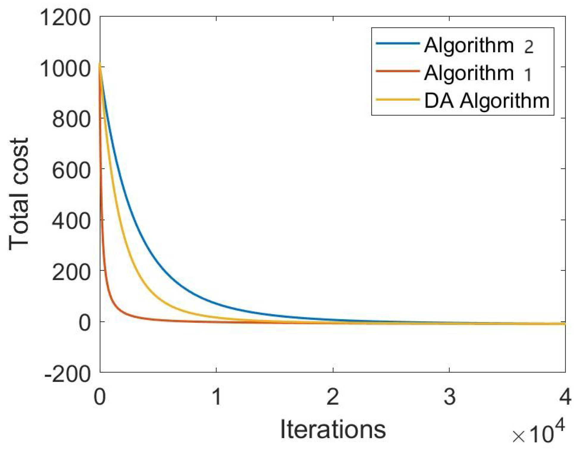
Next, the cost functions of all participants are accumulated and gradually decrease with algorithm iterations. As shown in Figure 4, it can be found that all three algorithms mentioned above minimize the cost function, and in comparison, using Algorithm 1 leads to the fastest decrease in the cost function.
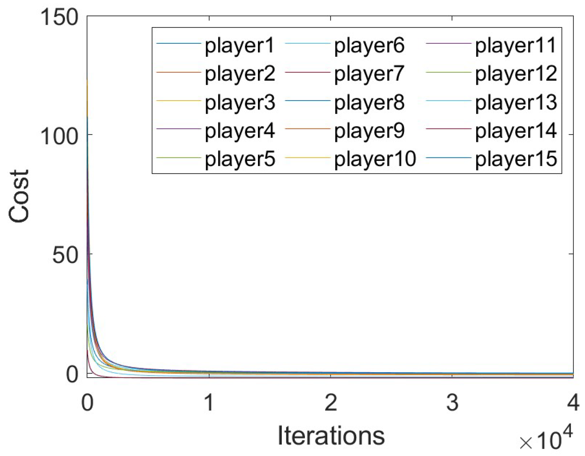
In order to clearly show how the algorithm works, the decreasing cost function of the 15 participants is shown in Figure 5, and it can be found that the cost function of each participant converges to the minimum value continuously and smoothly.
At the end of this section, the process of reaching agreement on the estimated variables x ^ of the global decision set x by the participants i N during the iteration of the algorithm is shown in Figure 1. As mentioned in this paper, the algorithm under local information elevates the decision vector latitude of the participants, and each participant has not only their own local decision x i = x i [ i ] R , but also an estimate of the other participants’ decisions x i [ i ] = col ( , x i 1 [ i ] , x i + 1 [ i ] , , x N [ i ] ) , where x j [ i ] denotes the estimate of participant i on participant j. Relatively, for each participant i, there exist N estimates of him, and we define this set as E , i.e., E = { x i [ 1 ] , , x i [ N ] } , let k be the number of iterations, if i { 1 , , N } , lim k V a r ( E ) = 0 , then it is proved that all decision makers reach agreement on the estimate of the global decision set, which is equivalent to knowing the global decision set.

6. Summary and Prospect

In this paper, we study algorithms for finding the GNE of noncooperative game problems for two different situations. In the case of global decision information, each participant can use the global decision set to minimize the cost function. In the case of partial decision information, participants need to estimate the global decision set and perform local optimization by estimating variables, while consensus dynamics with the Laplacian matrix ensures that the local estimations will reach the same GNE. This paper devotes an entire section to the derivation of Algorithms 1 and 2. In addition, we derive the step size condition for the convergence of the algorithm using the Gershgorin Circle Theorem and analyze the convergence of the algorithm under mild assumptions. Finally, we simulated both algorithms and compared them with the FB algorithm. This paper assumes that the objective function of each player is continuously differentiable, but in practical problems, there may be nonsmooth or nonconvex situations. Therefore, how to generalize the algorithm proposed in this paper to more general cases is a worthwhile research question. This paper only considers undirected connected graphs as the communication topology among players, but in real networks, there may be directed graphs or disconnected graphs. Therefore, how to analyze and design distributed algorithms that apply to these complex topological structures is a challenging problem. This paper only discusses the algorithm based on a synchronous update strategy, but in real networks, there may be asynchronous or random updates. Therefore, how to consider the impact of these update strategies on the performance and stability of the algorithm is a meaningful problem.

Author Contributions

Methodology, H.L. and Y.S.; Software, J.C., M.C. and Z.W.; Formal analysis, J.C., H.L. and M.C.; Investigation, J.C. and Y.S.; Resources, J.C. and Y.S.; Data curation, J.C., H.L. and J.T.; Writing—original draft, J.C.; Supervision, Y.S.; Project administration, J.C. and Y.S. All authors have read and agreed to the published version of the manuscript.

Funding

This research received no external funding.

Institutional Review Board Statement

Not applicable.

Informed Consent Statement

Not applicable.

Data Availability Statement

No new data were created.

Conflicts of Interest

The authors declare no conflict of interest.

References

  1. Facchinei, F.; Kanzow, C. Generalized Nash equilibrium problems. 4OR 2007, 5, 173–210. [Google Scholar] [CrossRef]
  2. Fischer, A.; Herrich, M.; Schonefeld, K. Generalized Nash equilibrium problems-recent advances and challenges. Pesqui. Oper. 2014, 34, 521–558. [Google Scholar] [CrossRef]
  3. Garcia, A.; Khatami, R.; Eksin, C.; Sezer, F. An Incentive Compatible Iterative Mechanism for Coupling Electricity Markets. IEEE Trans. Power Syst. 2021, 37, 1241–1252. [Google Scholar]
  4. Cadre, H.L.; Jacquot, P.; Wan, C.; Alasseur, C. Peer-to-Peer Electricity Market Analysis: From Variational to Generalized Nash Equilibrium. Eur. J. Oper. Res. 2018, 282, 753–771. [Google Scholar]
  5. Wu, C.; Gu, W.; Bo, R.; MehdipourPicha, H.; Jiang, P.; Wu, Z.; Lu, S.; Yao, S. Energy Trading and Generalized Nash Equilibrium in Combined Heat and Power Market. IEEE Trans. Power Syst. 2020, 35, 3378–3387. [Google Scholar] [CrossRef]
  6. Debreu, G. A Social Equilibrium Existence Theorem. Proc. Natl. Acad. Sci. USA 1952, 38, 886–893. [Google Scholar] [CrossRef] [Green Version]
  7. Rosen, J.B. Existence and Uniqueness of Equilibrium Points for Concave N-Person Games. Econometrica 1965, 33, 520–534. [Google Scholar] [CrossRef] [Green Version]
  8. Facchinei, F.; Kanzow, C. Generalized Nash Equilibrium Problems. Ann. Oper. Res. 2010, 175, 177–211. [Google Scholar] [CrossRef]
  9. Facchinei, F.; Pang, J.S. Nash equilibria: The Variational Approach. In Convex Optimization in Signal Processing and Communications; Cambridge University Press: Cambridge, UK, 2009. [Google Scholar]
  10. Yi, P.; Pavel, L. An Operator Splitting Approach for Distributed Generalized Nash Equilibria Computation. Automatica 2019, 102, 111–121. [Google Scholar] [CrossRef] [Green Version]
  11. Latafat, P.; Freris, N.M.; Patrinos, P. A New Randomized Block-Coordinate Primal-Dual Proximal Algorithm for Distributed Optimization. IEEE Trans. Autom. Control. 2019, 64, 4050–4065. [Google Scholar]
  12. Malitsky, Y. Golden Ratio Algorithms for Variational Inequalities. Math. Program. 2020, 184, 383–410. [Google Scholar] [CrossRef] [Green Version]
  13. Pavel, L. Distributed GNE Seeking Under Partial-Decision Information Over Networks via a Doubly-Augmented Operator Splitting Approach. IEEE Trans. Autom. Control. 2020, 65, 1584–1597. [Google Scholar] [CrossRef] [Green Version]
  14. Bianchi, M.; Belgioioso, G.; Grammatico, S. Fast generalized Nash equilibrium seeking under partial-decision information. Automatica 2022, 136, 110080. [Google Scholar] [CrossRef]
  15. Cai, X.; Xiao, F.; Wei, B. Distributed generalized Nash equilibrium seeking for noncooperative games with unknown cost functions. Int. J. Robust Nonlinear Control. 2022, 32, 8948–8964. [Google Scholar] [CrossRef]
  16. Aragón Artacho, F.J.; Campoy, R. Solving Graph Coloring Problems with the Douglas-Rachford Algorithm. Set-Valued Var. Anal. 2018, 26, 277–304. [Google Scholar]
  17. Lakshmi, R.J.; Rao, G.V.S. A Re-Constructive Algorithm to Improve Image Recovery in Compressed Sensing. J. Theor. Appl. Inf. Technol. 2017, 95, 5443–5453. [Google Scholar]
  18. Steidl, G.; Teuber, T. Removing Multiplicative Noise by Douglas-Rachford Splitting Methods. J. Math. Imaging Vis. 2010, 36, 168–184. [Google Scholar] [CrossRef] [Green Version]
  19. Egerestedt, M. Graph-Theoretic Methods for Multi-Agent Coordination; Georgia Institute of Technology: Atlanta, GA, USA, 2007. [Google Scholar]
  20. Giselsson, P.; Boyd, S. Linear Convergence and Metric Selection for Douglas-Rachford Splitting and ADMM. IEEE Trans. Autom. Control. 2014, 62, 532–544. [Google Scholar]
  21. Combettes, P.L. Monotone operator theory in convex optimization. Math. Program. 2018, 170, 177–206. [Google Scholar]
  22. Bell, H.E. Gershgorin’s Theorem and the Zeros of Polynomials. Am. Math. Mon. 1965, 72, 292–295. [Google Scholar] [CrossRef]
  23. Bauschke, H.H.; Combettes, P.L. Convex Analysis and Monotone Operator Theory in Hilbert Spaces, 2nd ed.; Springer Publishing Company: Berlin/Heidelberg, Germany, 2017. [Google Scholar]
  24. Peng, Y.; Pavel, L. Asynchronous Distributed Algorithms for Seeking Generalized Nash Equilibria Under Full and Partial-Decision Information. IEEE Trans. Cybern. 2020, 50, 2514–2526. [Google Scholar]
  25. Moschini, G.; Vissa, A. A Linear Inverse Demand System. J. Agric. Resour. Econ. 1992, 7, 294–302. [Google Scholar]
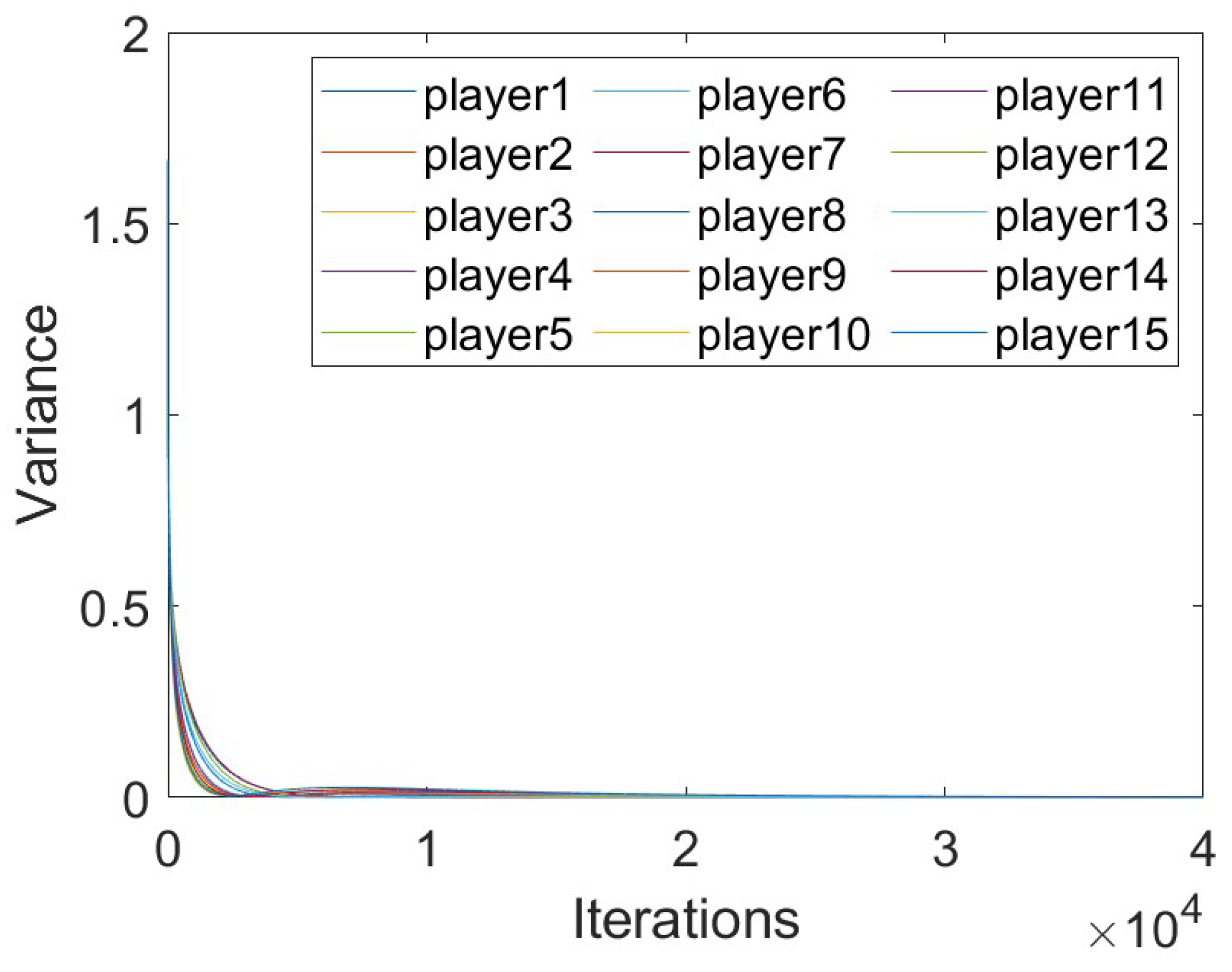
Figure 1. The figure shows the process by which all customers agree on the estimated value of GNE. The vertical coordinate is the variance, i.e., V a r ( x i [ 1 ] , , x i [ N ] ) , i { 1 , 2 , N } .
Applsci 13 07058 g001
Figure 2. The black arrows start at the client end and end at the router chosen by that client, and the clients at either end of the yellow arc are neighbors.
Applsci 13 07058 g002
Figure 3. The blue, red, and yellow curves indicate the convergence process of Algorithms 1 and 2, and DA algorithm, respectively.
Applsci 13 07058 g003
Figure 4. The figure shows how the sum of the costs of all customers changes under the action of the three algorithms. The ordinate is i = 1 i = N [ f i ( x i , x i ) + g i ( x i ) ] .
Applsci 13 07058 g004
Figure 5. The figure shows how the private cost per customer changes under the action of Algorithm 1. The ordinate is f i ( x i , x i ) + g i ( x i ) , i { 1 , . . . N } .
Applsci 13 07058 g005
Disclaimer/Publisher’s Note: The statements, opinions and data contained in all publications are solely those of the individual author(s) and contributor(s) and not of MDPI and/or the editor(s). MDPI and/or the editor(s) disclaim responsibility for any injury to people or property resulting from any ideas, methods, instructions or products referred to in the content.