Abstract
This study concerns the comparative investigation of two advanced lateral stability automotive controllers with respect to a commercial solution. The research aims to improve the stability performances achieved by a combined tracking of yaw rate and side-slip angle through the application of optimal efforts. The proposed solutions are based on Linear Quadratic Regulation and Sliding Mode Control, respectively. Both rely on the same approach for the control objective definition but differ from the action perspective. This solution involves the adoption of a differential braking actuation technique to deliver a desired yaw moment to the car body to track controlled states. Indeed, a sliding controller can also traction torques of hub-motor configurations as well as steering corrections, achieving vehicle stability and a driving response in accordance with the pilot’s intentions. Calibration and validation of the controllers are performed through a Hardware-in-the-Loop simulation rig, along with a real-time static simulator, performing different close-loop maneuvers to assess achievements in terms of lateral stability. Results show that both solutions ensure higher handling performances if compared to Non-controlled or Commercial-controlled vehicle scenarios.
1. Introduction
Ensuring the lateral stability of road vehicles is a fundamental task with respect to both passenger safety and driving comfort [1]. Moreover, the recent proliferation of By-Wires (BWs) and mechatronics systems in the automotive sector [2,3,4], as well as autonomous drive applications [5,6], are incentivizing researchers and designers in the development of innovative active safety controllers, for example, the Electronic Braking Distributor (EBD), Anti-Lock braking System (ABS), Traction Control System (TCS), Electronic Stability Program (ESP). Indeed, these systems exhibit a higher level of robustness with respect to conventional mechanical ones due to the reduced number of components and required maintenance, as well as improved reliability and fault-tolerance [7].
In the current literature, many solutions for ESP controllers have been proposed. This task appears extremely challenging due to the approximations and assumptions fundamental to implementing model predictive Real-Time (RT) control [8]. Recently, academic and industrial interest in the field of Torque Vectoring (TV) techniques is becoming more and more important in the automotive sector as it allows one to explore new opportunities concerning lateral stability control strategies [9]. Moreover, the availability of In-Wheel Motor (IWM) traction systems and BW technologies to consent to the implementation of non-conventional control methodology [10,11,12] appear extremely costly or even not feasible without the adoption of Electric/Electronic (E/E) devices.
In this work, the authors intend to propose two different lateral stability solutions to achieve higher lateral stability performances.
The first control strategy is developed and implemented in a Rear Wheel Drive (RWD) electric vehicle using an innovative Brake-By-Wire (BBW) architecture developed by Meccanica 42 S.r.l. [13]. This ESP is based on a tracking Linear Quadratic Regulator (LQR) able to find the optimal control gains to make the car follow the reference yaw rate and side slip angle. Compared to the State-of-Art (SoA) [14,15,16,17], which acts leading the side-slip angle and the yaw rate under a saturation limit, in this case, a continuous regulation on their values is assured by implementing not only the actual but also the reference yaw rate and side-slip angle values. Thus, by exploiting the brake actuators’ capabilities, it is possible to nullify the errors between the car and the dynamic reference model. In this way, the onset of instability is prevented, and a delay between the upper controller and the pressure controllers is not led. The output defined by the stability control is the total yaw moment that the car has to have to follow the ideal behavior. This total yaw moment is ensured by a developed logic that splits the moment into the four brake units. It is based on the moment sign, defining which side of the car to actuate. Then, according to the wheel adhesion condition, a percentage of braking torque is delivered to the wheel on that side. In addition, an algorithm that redistributes the control efforts as the wheel reaches its braking pressure limit is implemented to guarantee the yaw moment required by the control.
The second one was previously developed for IWM-driven Electric Vehicles (EVs) equipped with BW systems [18,19,20] and is based on Sliding Mode Control (SMC) methodology. This particular vehicle layout has been the subject of numerous studies [21,22,23,24]. In the available SoA, we can find many papers proposing a coordinated control between steering and differential torque allocation to achieve higher stability performances [25,26,27,28,29,30,31]. The proposed solution provides combined actions between the Steer-by-Wire (SBW) system and torque allocation to ensure the tracking of side-slip angle and yaw rate r. Optimal control signals, i.e., adjusting yaw moment and correcting steering angle, are calculated through a Lyapunov candidate, which leads the derivatives of the controlled state to converge to 0 asymptotically. The controller is composed of three sub-systems: (1) High-level layer, which gathers information from the vehicle info bus to define the control objectives, estimated through a model-based approach; (2) Intermediate-level layer, dedicated to calculating the desired control actions; (3) Low-level layer, which generates the reference signals for the actuators. With respect to previous work based on Sliding Mode strategies [32,33,34,35], typically using separated sliding surfaces that decouple the control dynamics, this algorithm relies on a 2 dimensions model for the states control. These challenges are well-known and established lateral stability SMC methods adopt a single sliding surface. Moreover, the application of desired yaw moment is based on Moore–Penrose Pseudo-inverse innovative criteria [12,36] to solve a multi-Degree Of Freedom (DoF) problem for over-actuated systems. This allows us to achieve both vehicle stabilization and a driving path that is in accordance with the driver’s intentions. Even if the controller is developed for 4 Wheel Drive (4WD) architectures with independent traction wheels, the adopted approach ensures fundamental features, which consent to flexibility and portability of the solution with respect to different vehicle layouts and applications.
To assess the goals of this work, a simulation campaign of closed-loop maneuvers is performed by comparing proposed controllers with a reference commercial ESP on a driving simulator. This Hardware-in-the-Loop (HiL) system is composed of a concurrent PC, in which reside the RT vehicle model and the control algorithms; a commercial braking unit and EPSiL steering bench; and driver interface devices, for example, pedal and steering wheel.
2. Control Strategies
Controlling the lateral behavior of automotive vehicles is fundamental to achieving higher safety and comfort levels for passengers. Typically, Electronic Stability Controls (ESCs) act on brake actuators to prevent undesired operative conditions, such as under-over steering and rollover. The recent availability of BW systems opens the way to the adoption of more sophisticated control policies, able to exploit new possibilities. Indeed, BBW actuators consent to the application of different braking torques on each wheel, increasing the overall yaw moment which can be applied to the vehicle body. In addition, SBW can be easily interfaced with a high-level Control Unit (CU), introducing additional steering angle and assisting the driver during dangerous and risky maneuvers. In the next subsections, the proposed model-based control methodologies are described in detail, which rely on the LQR theory and SMC approach. Both strategies have in common the control objective definition, which is explained here.
Assumption
A single-track model with 3-DoF in longitudinal x, lateral y, and yaw motion directions is considered. and are the longitudinal and lateral forces generated in the tire-road contact patch; is the front wheel steering angles; and are longitudinal and lateral speed; is the side-slip angle; a and b are the front and rear wheelbase. In all the equations, the same convention is adopted in which stands for front or rear axle, respectively.
The controllers are based on the following assumptions, fundamental to ensure the validity of the adopted modeling approach, both concerning dynamics and kinematics variables:
- (a)
- Steering angle is small: < 10 deg;
- (b)
- Vehicle longitudinal speed is constant: ;
- (c)
- Tire slip angles are small: deg;
- (d)
- Tire cornering stiffness is known and constant: .
Small tire slip angle and constant cornering stiffness , instead, are abstracted through (3) and (4), assuming a linear behavior of the wheel’s lateral forces with respect to side-slip angles .
Vehicle Dynamics
Lateral and yaw motion dynamics are described by (5), where m is the mass, lateral acceleration, and the external yaw moment, typically applied through differential torque allocation between left and right wheels.
This approach is fundamental to defining the state space of the dynamic vehicle behavior.
Target Vehicle Kinematics
Desired side-slip angle (7) and yaw rate (8) appear linearly dependent by if it is assumed that the front steering vehicle is in steady state conditions. Indeed, in this situation, (9) is the steering angle for negotiating a curve radius R, with (10) being the vehicle under-steer gradient .
However, desired states (7) and (8) cannot always be obtained, for example, in poor tire-road friction conditions. For these reasons, target states must be bounded, considering safety factors. If the lateral acceleration at the vehicle Centre of Gravity (CoG) is defined by (11), it should be upper bounded by the friction coefficient .
Assuming that and its derivative are small, the second and the third term of (13) are negligible, while the first one dominates. Considering a safety factor of , the target yaw rate can be bounded by (14), as described in (15). In this way, it is supposed that the second and third elements of (13) contribute only 15% to the total lateral acceleration.
Limiting the target side-slip angle is also very important because higher values of lead the tires to lose their linear behavior, approaching the limit of adhesion. Thus, it is upper bounded by the empirical relation (16), as is visible in (17).
2.1. Linear Quadratic Lateral Tracking Control
The considered BBW architecture is able to continuously track four different target pressures, to be assigned to each wheel. This allows the development of a high-level tracking control system that ensures stability and safety using an LQR approach. To achieve this, the controller aims at the direct regulations of the actual yaw rate and side-slip angle of the vehicle expressed by the single-track dynamic vehicle model, while the reference states rely on the ideal kinematic model described in the previous section. Therefore, the outputs of the optimal control are the errors between the actual and reference states, which are minimized by delivering to the vehicle body a desired yaw moment. This is applied through continuous and independent braking actuation actions on the wheels.
2.1.1. Controller Structure
The controller architecture, shown in Figure 1, comprises a reference model, an LQR controller, and a brake pressure split logic. According to the RT conditions, the control quantities have been discretized with a sample time of 0.001 s. The reference model has the task of providing the desired values of the side-slip angle and yaw rate. It receives as inputs the driver demands: steering wheel angle and desired vehicle longitudinal speed. Modeling the car through the formulations shown in Target Vehicle Kinematics section, the controller allows one to track the ideal vehicle behavior, leading the side-slip angle and yaw rate errors to decrease. This ensures improved lateral stability performances. To ensure that the vehicle achieves this condition, a logic that allocates braking pressures to each wheel’s actuators is implemented.
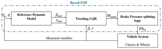
Figure 1.
LQR-Stability control structure.
2.1.2. LQR Controller Design
The main objective of this controller is to ensure the vehicle follows an ideal kinematic behavior, achieving increased lateral stability and optimal driving performance. During a maneuver, lateral and yawing dynamics of the vehicle change over time according to initial drive conditions imposed by the driver. To extrapolate the inner maneuverability characteristics and to independently actuate the wheel’s brakes to compensate for under-steering or over-steering vehicle behavior, the steady state values of yaw rate and side-slip angle are calculated by (15)–(17). Since the reference states vary while the vehicle is in motion, they must be represented in a state-space form to be implemented in a control structure. This can be conducted by defining the gradients of and using (18), where s is the Laplace variable, and is the time constant:
Therefore, the state-space of these transfer functions is composed of side-slip angle and yaw rate as states. This represents the reference that the vehicle should follow. Instead, the actual values of yaw rate and side slip angle are modeled as described in the Vehicle Dynamics section. Thanks to this, a State-Space of the vehicle is implemented, where (19) are the side-slip angle and the yaw rate, and the input (20) is the desired total yaw moment.
The control task is composed of a given system and a feasible target : the aim is to design a compensator of the form which ensures . This is known as Trajectory Tracking Problem. To design a controller capable of solving this type of problem, the vehicle State-Space model is concatenated with the reference ones, achieving a new dynamic model described by (23)–(26). In this way, it is possible to define the outputs as the errors between the actual and the desired values of the states. Therefore, the goal of the control is to establish the input which minimizes these errors.
Once the dynamic model is specified, the stability is ensured by the Linear Quadratic Regulator, which is an optimal control. This strategy minimizes a quadratic cost function (27) by weighing the output, Y, and the input, u, by the matrices Q and R, respectively, and solving the Riccati Equations (28) and (29). In this way, specific gains, K and , are defined for each actual, x, and reference, , state to lead the input (30).
The LQR control is, as already mentioned, an optimal control, i.e., it is optimally referred to as a specific performance index. In this case, the index is the cost function (27), whose minimization allows us to solve the trajectory tracking problem by definition of the control law (30), which at this point is applied in RT.
2.1.3. Brake Pressure Splitting Logic
This logic aims to ensure that the total moment required is reached: firstly, selecting if the right or left wheel side needs to be actuated in accordance to the sign of the input moment; and then defining how much each wheel has to be braked facing the problem of braking pressure saturation limit.
To identify the wheel to be actuated, a selector based on the understeering and oversteering behavior is adopted: when the vehicle is understeering, it goes to a greater trajectory than that set by the driver. To compensate for the error in the trajectory and linearise the vehicle behavior to the driver’s input, a braking force must be applied on the inner rear wheel. On the other hand, when the vehicle is oversteering, to compensate for the development of the vehicle on a lower trajectory, the outer front wheel must be braked (31)–(34). In these equations, the symbols represent the brake moment, where index i inherits the same convention described in the previous Section 2, while indicates the left or right wheel, respectively.
Thus, it is possible to reduce the lateral slip by adding a longitudinal slip component.
From the torques found, through the rotational balance (36), the braking pressure delivered to each wheel is defined (35).
The BBW system saturates the brake caliper pressures to a maximum of 150 bar. This constraint could limit the braking force of the wheel, not ensuring achieving the moment requested. For this reason, a logic that redistributes the pressure on the wheels is developed, consisting of the following steps:
- Checking if the wheel reaches the saturation limit;
- Definition of the pressure quantity by which the saturation limit is exceeded;
- Subtraction of this quantity from the wheel of the other side ensures the allocation of the control yaw moment.
In addition, the EBD-ABS logic explained in [37] has been added to ensure that the wheels do not lock up.
2.2. Sliding Mode Lateral Stability Control
This lateral stability solution is based on the Sliding Mode methodology. The objective is the direct control of vehicle side-slip angle and yaw rate r by the application of corrective steering and TV efforts. The SMC-based ESP algorithm, whose simplified block diagram is visible in Figure 2, is developed on three different layers, depending on the task the sub-controller must accomplish:
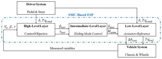
Figure 2.
Block diagram of the SMC controller.
- High-level layer: which defines the control objective according to driver intention and vehicle states, for example, longitudinal speed, side-slip angle, yaw rate;
- Intermediate-level layer: consisting of a first-order Sliding Mode Controller;
- Low-level layer: devoted to the generation of the control references for the actuators, i.e., SBW, BBW, and traction motors.
In-depth information about each controller layer can be found in the following chapters. The proposed solution respects fundamental features to exhibit portability and flexibility properties: scalability, abstraction, parametrization, modularity, and RT capability. This allows the controller to be implemented for different vehicle architectures, for example, Internal Combustion Engine (ICE), EV, FWD, and 4WD.
2.2.1. Modeling Approach: High-Level Layer
This control layer relies on ideal and simplified vehicle equations to define the control objectives [8]. It combines information from sensors and estimators, thereby generating reference control signals. As already pointed out, the SMC aims at the direct control of the vehicle’s side-slip angle and yaw rate. It is important to highlight that target states rely on ideal kinematic vehicle behavior, while the High-Level layer is based on dynamic relations. A four-wheel vehicle model with 3-DoF is considered (Figure 3). and are the longitudinal and lateral forces; is the front wheel steering angles; is the tracks.
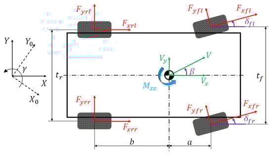
Figure 3.
Three DoF Vehicle Dynamic Model.
Left and right wheel steer angles are supposed to equal . For further improvements, this assumption can be removed by considering different steering angles for right and left front tires. This leads to the increased dimension of the state space model.
Rearranging (6) and making explicit the external yaw moment as in (37) allows us to obtain the state space model (38) of the controlled variable , with .
This modeling approach could also be applied to a front and rear wheels steering vehicle by increasing the dimension of matrix B to 3 × 2 in (38), with control input .
Considering the vector and the assumption (39), with k the k-th sampling step at a rate of , the model of (40) is valid and corresponds to the state space model of the desired side-slip angle and yaw rate, obtained by differentiation of the kinematic Equations (7) and (8).
A second order transfer function (41) is used both for the target side-slip angle and yaw rate to include the real dynamic behavior of the vehicle, which exhibits smoother conduct with respect to the one calculated in (7) and (8).
To ensure x asymptotically converge to , the modeling approach described in this section is fundamental. Indeed, optimal control effort calculated by the Intermediate-level layer using SMC requires the knowledge of actual and target-controlled states. The control objectives are calculated at each time step, fixed in this case at 0.001 s to update the current desired path behavior. This allows the calculation of optimal control efforts.
2.2.2. Control Theory: Intermediate-Level Layer
The Intermediate-level receives the control objectives from the upper controller, along with the driver inputs and vehicle states, to define desired wheel steer demand and equivalent yaw moments to be applied to the vehicle.
To lead the states and r to converge to the target values, a first-order Sliding Mode Controller is proposed. Its action is typically composed of feed-forward impedance control terms (based on model considerations) and feed-back compensation terms (similar to a Proportional-Integral-Derivative control method). Optimal control input is selected according to (42), ensuring that desired states error tend asymptotically to 0, where target states error is used for the proportional and integral compensation.
It is worth nothing to note that matrix of (41) is non-invertible, so a pseudo-inverse operator is used. The Lyapunov stability of the SMC-based ESP is guaranteed by the function candidate (43) [23], whose convergence is ensured by condition (44).
Selecting k, , and according to (46), the Lyapunov stability is proved. However, to obtain the best stability control performances from this controller, the multiple gains have to be tuned properly. This process was carried out during the preliminary test phases.
2.2.3. Effort Application: Low-Level Layer
Most of the current control solutions use differential braking between the left and right wheels to induce a correcting yaw moment on the vehicle chassis. However, non-conventional vehicle architecture, such as direct wheel-driven cars, allows one to benefit also from traction torques, independently delivered to each wheel. Indeed, in more sophisticated vehicle layouts, the availability of multi-quadrant electric motors (IWM) or active differential consent to take advantage also of traction torque, resulting in a higher value of applicable momentum around the vehicle’s z-axis. Moreover, the presence of SBW and BBW systems ensures simple interfaceability with higher-level CU, allowing the implementation of advanced and complex control solutions.
Even if optimal control signals (42) secure the controlled states converge to desired ones, an allocation problem still need to be solved. Indeed, the controller should stabilize the vehicle as well as produce control effort that is in accordance with the driver’s intention, keeping unaltered the driving path.
To avoid the typical chattering problem of the Sliding Mode controller [24], saturation is adopted in the definition of the control dead zone. Note that using these functions to deal with SMC output discontinuities could be detrimental since the controller formulation loses its robustness properties [33]. To solve this, specific smoothing transfer functions are used. Adopted criteria are the values of the state errors and vehicle longitudinal speed. This solution provides a useful tool to avoid the fast transient yaw moment demanded by the upper controller during abrupt cornering maneuvers. This leads to the use of relatively high control gains while averting undesired spikes during the wheel torque allocation phase.
This low-level controller is parametrized to be easily applied to different traction architectures. This ensures the portability and flexibility of the whole proposed strategy, allowing the application of advanced TV techniques, regardless of vehicle layout.
Steer Command
Optimal steer angle is applied as a correction with respect to the desired trajectory: it should not directly overwrite the driver command. For doing so, is limited to 10% of the steering angle command to avoid deviation, which could lead to unpredictable vehicle dynamics. Indeed, during fast transient phases, a greater wheel steering angle correction can bring the tires outside the linear behavior boundaries, saturating the available friction in the contact patch (high lateral and longitudinal slips). Moreover, the rate of the steering correction is limited to 1500 deg/s to not exceed the maximum driver capability of the steering angle speed application [38].
Yaw Moment
The task of this controller is to map the desired yaw moment into equivalent torque demand for each wheel. In this case, the desired is applied to the vehicle using an advanced TV technique. However, this approach contemplates a constrained control problem because of the multi-DoF solutions which are available. Indeed, independent wheel torque control implicates 4-DoF. This leads to possible solutions [9]. For this reason, an optimal allocation strategy based on Moore–Penrose Pseudo-inverse is proposed [18], where TV efforts are limited to the maximum deliverable torques of each wheel. Even in this case, a good trade-off between vehicle stability and driver intention must be satisfied.
The optimal yaw moment calculated by (42) is the external yaw moment defined in (37). However, some modifications are assumed. Firstly, the last term of (37) is neglected. This assumption is coherent with the proposed testing procedure and condition . As will be explained later, the maximum road angle during the reference maneuvers is about 6 deg, which limits the contribution of the sine component to a maximum of 10%. For further activities, this term can be accounted. Moreover, the allocation problem is formulated to consider different steering angles of left and right front tires, and , respectively. This is because the simulation environment makes available these values, so it is possible to consider a component that ensures a higher knowledge of vehicle dynamics. Therefore, the correcting yaw moment imposed on the torque allocator is the one described by (47).
The problem formulation is given by (48), where: is the vector of the difference between wheel torque demanded by the driver and the ESP torque command (with for front left, front right, rear left and rear right wheel); and are the front and rear wheel radius, respectively. Driver torques are established by the EBD, which observes the brake and throttle pedal travels, modifying these values according to longitudinal load transfer. The two rows composing (48) actually reduce the overall control solutions to . One DoF is removed by imposing the application of , ensuring the desired lateral behavior of the vehicle (first row); the second row corresponds to the need for demanding wheel torques in agreement with the driver’s purpose, which removes another DoF. A Moore–Penrose pseudo-inverse methodology is adopted to select the optimal solution among all those available. The TV technique is applied to solve (49), with the pseudo-inverse matrix of L.
This solution minimizes norm 2 of the functional cost (50).
The allocation process must also respect the actuator’s constraints. Indeed, (50) is solved in 4 sequential k-steps to be compared with the upper and lower torque limit of the reference wheel. In each step, the k-th element of is checked with respect to the constraints of the tire motor and brake. If these are exceeded, the value is saturated to the limit, and the solution is recalculated in the following -step, excluding from the system the row related to the k-th wheel, as defined in (51). A maximum limit of 1000 Nm for each wheel is imposed. After this stage, a single optimal solution is found, removing the last 2 DoF.
It is important to point out that the longitudinal stability task, i.e., front/rear axle longitudinal effort distribution, anti-slip and anti-spin regulations, the burden on dedicated controllers (EBD, ABS, and TCS), which are already implemented in the vehicle model.
3. Real-Time Driving Simulator
To test the stability performances allowed by the proposed ESP strategies, the controllers are evaluated in the RT driving simulators of Figure 4. Using a Hardware in the Loop (HiL) test rig allows us to understand which impact these solutions introduce, both on vehicle behavior and driver perception, supposing real driving conditions. The experimental activity has been carried out on the static simulator supplied by Meccanica 42 S.r.l., equipped with a steering wheel, brake pedal, and throttle pedal as human–interface devices. It is composed of three main parts, as described in Figure 5:
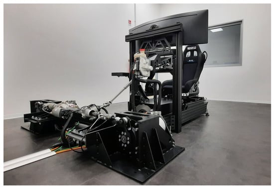
Figure 4.
Meccanica 42 S.r.l. real-time driving simulator.
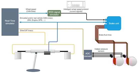
Figure 5.
Static simulator setup.
- The Real-Time simulator: consisting in a concurrent-RT machine, which manages the simulation environment along with the vehicle model. For non-disclosure reasons, the detailed specifications of the benchmark Use Case (UC) cannot be described. However, it is implemented with stability CU, i.e., EBD, ABS, TCS, and commercial ESP solution. Moreover, it is assumed that the vehicle’s RWD powertrain is actuated to an active differential transmission system;
- The EPSiL steering bench: reproducing the real behavior of the steering system, including the Electric Power Steering system (EPS) and a steering wheel;
- The Braking unit: a by-wire system that includes all the components of a real disc brake plant with independent control of each wheel caliper. Moreover, a virtual sensing regulation loop is considered.
3.1. Epsil Steering Bench
The EPSiL steering bench integrates a complete steering system implemented in a HiL driving simulator. Two torque motors and transmissions act directly on the tie-rods of the real steering system by means of a rocker, accurately reproducing the kinematic movement of the suspensions. With this architecture, the rig is able to reproduce all the forces acting beyond the xy plane, improving the reliability of the vehicle model by accurately reproducing the actual efforts insisting on the car chassis. The tie-rods, equipped with load cells, rack, EPS, steering column, and steering wheel, are integrated into the system. The described steering layout replicates exactly the commercial solution equipped on the simulated vehicle. The steering bench is included in the simulation loop, enhancing the driving experience and providing the necessary tool for steering virtual development. Indeed, through CAN connection, it is possible to observe the feedback signals and tune the parameters of the EPS parameters to calibrate the system, while the driver can assess the effect of each modification on multiple testing conditions. The unit proved itself capable of accurately reproducing real-vehicle tie-rod forces, resulting in an efficient and reliable steering feeling [39].
3.2. Braking Unit
A commercially available brake-by-wire system, known as MKC1 produced by Continental GmbH, has been implemented on the simulation rig. The installation layout is described in Figure 5. The stock brake plant is mounted on the simulator. It includes the brake tubes (with the correct diameter and length), which are connected to the electro-mechanical units of 4 independent stock brake calipers, acting on the original brake discs. The brake pedal is directly integrated into the unit, and it constitutes the main braking unit driver-machine interface device.
The brake unit communicates through the communication lines using a Control Area Network (CAN) protocol, receiving all the signals that are usually exchanged on real vehicles (e.g., from IMU), simulated by the model on the RT computer. In addition, this unit needs intelligent wheel speed signals via a direct communication line. For this reason, virtual wheel speed sensors have been implemented, which convert wheel speed (received via CAN from the RT machine) to the typical signal type provided by intelligent wheel speed sensors [40].
Finally, four pressure sensors have been installed on the calipers, and their signals are sent back to the vehicle model via an EtherCAT measurement line, closing the loop and controlling the vehicle deceleration after a brake demand from the driver.
The unit functionalities have been tested in [41], comparing the responses and behaviors on the static simulator with respect to a real vehicle, proving its effectiveness on a previously validated vehicle model.
4. Simulation Results
4.1. Offline Test Campaigns: Tuning of the Controllers
Before the testing phase in the HiL system, the controllers are first implemented in the co-simulation environment between MATLAB and VI-Grade. In particular, the control solutions are developed in Simulink, while the vehicle model resides in CarRealTime. Thus, a preliminary test campaign aimed at tuning the multiple gains is conducted for both LQR and SMC solutions. In addition, a recursive optimization algorithm is used to identify the tire cornering stiffness and of the vehicle model. These are assumed constant and known for the control objectives calculations but appear non-linear for the tire modeling approach adopted in VI-Grade, which relies on Pacejka equations [42].
In this stage, a standardized open-loop cornering maneuver is replicated: the Step Steer test. It is executed in accordance with the ISO7401:2003 standard, also known as the Lateral Transient Response test method. However, there is still the risk that the gains are tuned optimally only for these specific test boundary conditions, showing poor performances when the vehicle operates in quite different scenarios with respect to the one considered during the optimization phase. To avoid the tuning process being affected by these problems, multiple functional costs (52) are evaluated, where and are real and desired variables, respectively. Investigated vehicle states are lateral displacement y, lateral acceleration , yaw rate r, and side-slip angle .
4.2. Online Test Campaigns: Performance Evaluations
In this phase, a driver replicates some reference cornering tests using the above-described RT driving simulator through the HiL interface system. To assure reliable comparative metrics, reference closed-loop maneuvers are repeated supposing four scenarios, in which the vehicle model is alternatively implemented with different controlling techniques:
- Non-Controlled Scenario: in this case, the vehicle is driven without the assistance of any kind of lateral stability controller. Thus, it was possible to establish inner vehicle maneuverability and test the driver’s capabilities. Many free driving tests are conducted to identify the limit of controllability;
- Commercial-Controlled Scenario: tests are conducted with the Continental GmbH proprietary ESP controller. The strategy, from our side, is completely unknown. However, we can make some assumptions, supposing the control technique is advanced and represent the SoA of the industrial ESP solutions, which is actually implemented on different vehicles in the market.
- LQR-Controlled Scenario: the Linear Quadratic lateral Tracking Control is tested, thanks to the RT co-simulation capabilities of the virtual environment, between MATLAB Simulink and VI-Grade;
- SMC-Controlled Scenario: here, the Sliding Mode Lateral Stability Controller is investigated, exploiting the same control rig from the previous scenario (ESP in MATLAB Simulink and vehicle model in the VI-Grade).
The investigated reference maneuvers are repeated many times, selecting the results which appear more comparable. Indeed, to ensure reliable comparative metrics it is fundamental to reproduce the close-loop test as similar as possible. Selected cornering tests are summarized in Table 1.

Table 1.
Investigated reference maneuvers.
However, boundary conditions specified by the related standards are modified to guarantee more severe conditions in terms of stability performances. This is useful to highlight the results [43]. Indeed, due to the excellent handling capabilities of the vehicle model, using the reference operative scenario produce no unstable behavior, making it difficult to assess the improvements related to the investigated controllers. The main contributions of ESP systems concern the stabilization of vehicle trajectory and desired driving path when unstable Non-Linear (NL) behavior onset.
To ensure an easy understanding of the results, output plots are presented for LQR and SMC, compared with Non-controlled and Commercial-controlled scenarios.
4.3. Ramp Steer
The Slowly Increasing Steer (SIS) test is used here to observe the linear behavior between the steering angle and the lateral response of the vehicle in the different controlling situations. The vehicle is driver at 120 km/h with a steering angle linearly increased from 0 deg to 270 deg. Even in this case, the test is conducted for right and left cornering directions. The ratio of applied steering angle is slow to assure steady-state behavior, avoiding abrupt deviation in the maneuver until the stability margin is reached, for example, the manifest of wheel side-slipping, non-linear, and undesired behavior. The SIS test was useful to establish the upper and lower limits of controlling interventions regarding actuator systems, i.e., brakes, motors, and steer.
4.4. Step Steer
Inspired by the ISO 7401:2003 standard, a Step Input test is performed in both directions: left and right turning. In respect to the reference maneuvers, this one is carried out in closed-loop conditions with an initial longitudinal speed of 150 km/h and a wheel steering angle of 90 deg. It is worth noting that this lateral test actually exhibits a ramp steering command. Indeed, the human driver cannot apply an instantaneous angle to the steering wheel [38]. However, the steering rate is high enough to produce a rapid cornering maneuver, letting us investigate the vehicle’s fast transient behavior.
Results of Figure 6 clearly show that both controllers succeed in tracking yaw rate and side-slip angle if compared to Non-controlled and Commercial-controlled scenarios. Controlled state errors are reduced for LQR and SMC solutions thanks to the application of optimal control efforts, visible in Figure 7 and Figure 8.
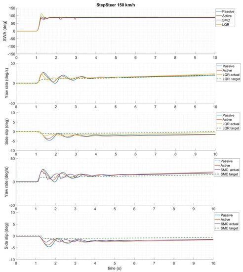
Figure 6.
Evaluation of the states tracking performances in case of Non-controlled (Passive), Commercial-controlled (Active), LQR, and SMC-controlled scenarios, in a Step Steer maneuver at 150 km/h and with 90 deg steering wheel angle.
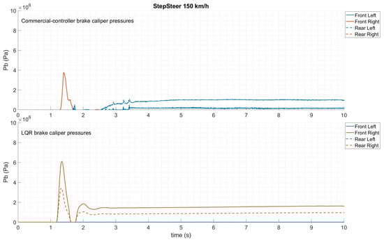
Figure 7.
Evaluation of the four brake caliper pressures in the case of Commercial-controlled and LQR-controlled scenarios, in a Step Steer maneuver at 150 km/h and with 90 deg steering wheel angle.
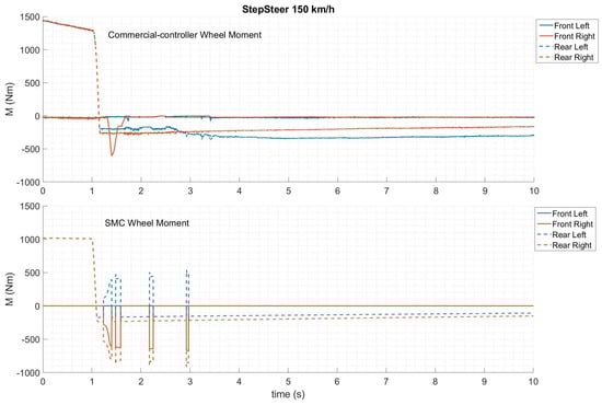
Figure 8.
Evaluation of the four-wheel moments in the case of Commercial-controlled and SMC-controlled scenarios, in a Step Steer maneuver at 150 km/h and with 90 deg steering wheel angle.
It is interesting to highlight that both proposed controllers apply different torque vectoring efforts with respect to the benchmark ESC. In the first stage (at about 1.5 s), all the stability systems perform quite similarly, despite the fact that SMC and LQR solutions show higher control actions. In the steady-state phase of the maneuver, indeed, controllers actuate the wheels on the opposite side with respect to the Commercial-controlled scenario. This is due to the fact that the developed solutions aim at the control of side-slip angle, in addition to yaw rate, which typically is the sole control objective of wide diffused ESC in the market.
4.5. Sine Steer
A sine path wave of 90 deg on the steering wheel is realized by the driver while traveling at 150 km/h to evaluate the responsiveness of the controlling techniques during this test. These maneuvers allow us to investigate the correctness of the implemented dead zone on the states errors since both yaw rate and side-slip consecutively cross 0 values. In the top plot of Figure 9, the steering angle imposed by the driver is visible for the different scenarios. For the SMC-Controlled solutions, the impact of the steering correction control technique is shown.
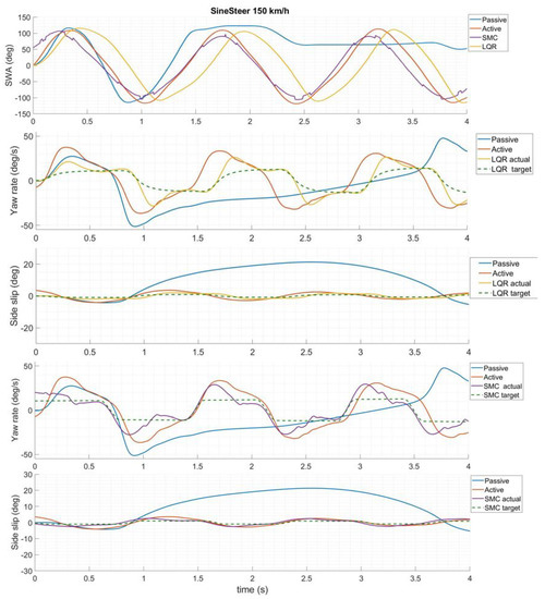
Figure 9.
Evaluation of the states tracking performances in case of Non-controlled vehicle (Passive), Commercial-controlled vehicle (Active), LQR, and SMC controlled scenarios, in a Sine Steer, maneuver at 150 km/h and a 90 deg of steering wheel angle amplitude.
Even in this case, the proposed controllers perform quite well with respect to the task of tracking the controlled states. In Non-controlled solutions, the vehicle is unstable, while for LQR and SMC scenarios, both vehicle yaw rate and side-slip angle are controlled by active torque distributions effort of Figure 10 and Figure 11, exhibiting improved stability performances even respect to Commercial-controlled scenario.
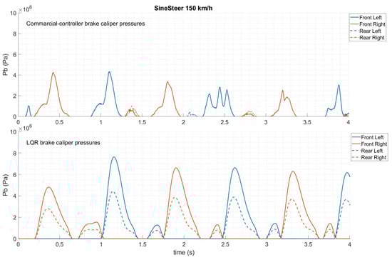
Figure 10.
Evaluation of the four brake caliper pressures in the case of Commercial-controlled vehicle and LQR controlled in a Sine Steer maneuver of 150 km/h and 90 deg steering wheel angle.
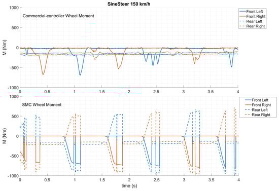
Figure 11.
Evaluation of the four-wheel moments in the case of a Commercial-controlled vehicle and SMC controlled in a Sine Steer maneuver of 150 km/h and 90 deg steering wheel angle.
As for the Step Steer test, LQR and SMC control actions show higher control effort values with respect to the reference ESP controller. This leads to improved tracking performances of the controlled states, especially for the side-slip angle, achieving a higher safety margin.
4.6. Lane Change
A single Lane-Change maneuver test is conducted to determine vehicle stability aspects subjectively. With respect to previous tests, this is the only one which is specified closed-loop by the reference standard (ISO 3888). The vehicle is driven at 150 km/h, and a steering path is imposed by the pilot to obtain a lateral displacement of about 3 m. Subsequently, another steer command is applied to re-orient the car in the longitudinal direction. Figure 12 shows the driving path performed by the vehicle during the maneuver and the vehicle’s longitudinal speed.
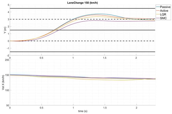
Figure 12.
Evaluation of the trajectory and longitudinal speed in case of Non-controlled vehicle (Passive), Commercial-controlled vehicle (Active), SMC, and LQR controlled, in a Lane Change maneuver of 150 km/h and a lateral displacement of about 3 m.
It is interesting to note that the LQR scenario trajectory exhibits a slight overshoot in the lateral displacement with respect to the center line, with a reduced speed with respect to other scenarios. SMC, indeed, tracks desired trajectory with a smoother behavior. This is due to the fact that sliding control adopts accelerometric criteria with fixed dead zones, reducing the control effort when approaching target states. For that concerning the speed, the sliding mode solution allows one to perform the reference maneuver in accordance with the driver’s intention, maintaining the entrance longitudinal speed by the exploitation of the traction forces of the powertrain.
5. Conclusions and Future Developments
The evaluation of two different lateral stability controllers for automotive vehicles has been performed, comparing the two solutions with a benchmark ESP solution already used in car models actually in the market. Both Linear Quadratic Regulator and Sliding Mode Control aim at the direct regulation of the vehicle’s yaw rate and side-slip angle to achieve stability improvements with respect to the conventional solution, based solely on yaw rate tracking.
In this work, the tracking and stability capabilities of LQR and SMC strategies are investigated. The controllers share the same algorithm for the control objective definitions, so the output comparability is ensured by the same reference modeling approach. However, the proposed solutions differ from the optimal control effort calculations aspect. In its most common configuration, the LQR controller can apply a yaw moment to the car body with a differential braking technique to stabilize the trajectory. The SMC controller is developed respecting important features to ensure flexibility and portability of the strategy with respect to quite different powertrain architectures. The best performance of this controller can be obtained by considering independent electric hub motors for 4WD vehicles, which guarantee a higher applicable yaw momentum thanks to the easiness of 4-quadrant torque control, enabling the exploiting of traction forces. In addition, the 2-dimension sliding surface formulation enables the option to apply even steer angle corrections.
The assessment is performed in a co-simulation environment exploiting an RT driving simulator hardware system, which allows a driver to perform different reference maneuvers, piloting the vehicle through steer and pedal interface devices. The maneuvers are inspired by standard cornering tests to assess achievement in terms of lateral stability using a Human-in-the-Loop approach. This means that a control rig composed of the vehicle, environment, and driver is required. Evaluating the stability performances in this kind of test is very challenging since there is a significant interaction between these elements. Therefore, the results are a combination of inner car handling dynamics and driver road-holding capabilities. To highlight the outputs, more difficult operative situations have been simulated with respect to the boundary conditions specified by the ISO regulations. Performance achievements related to standardized vehicle speed and steer command are quite negligible since the vehicle operates in a steady-state mode. Instead, bringing the vehicle near to unstable conditions allows us to make more evident the effects of the controllers, which aims at leading the vehicle back to a linear behavior. The executed cornering maneuvers could show some gaps between each other in terms of steering amplitude and rate, as well as speed tracking. This is due to the inability of any human driver to ensure the perfect repeatability of the tests. However, to mitigate this aspect, multiple tests are conducted, comparing the most similar ones.
The simulation campaign consists of a preliminary off-line test phase, in which controllers are tuned. Ramp Steer was fundamental for the definition of the effort constraints, adopted as saturation limits for brake pressures and wheel torques. Instead, Step Steer tests with low lateral acceleration were useful for the tuning of parameters related to control objective definitions (e.g., tire cornering stiffness).
The on-line test phase refers to standard cornering maneuvers in HiL configuration. Results highlight as both proposed control strategies enable improved performances with respect to Non-controlled and Commercial-controlled vehicle scenarios. Indeed, actual yaw rates and side-slip angles exhibit lower errors with respect to target values using LQR and SMC stability program solutions.
In particular, in the Step Steer maneuver (Figure 6), it is evident how the tracking efforts exhibit different control actions between developed ESP solutions and the Commercial one, achieving better stability and dynamic performance of the car. This is also shown in the Sine Steer test of Figure 9. Furthermore, the need for stability control is essential: the driver with a Non-Controlled vehicle is unable to perform the maneuver without losing control of the car; instead, the configuration with an ESP ensures one can maintain stability and maneuverability. The differences between the proposed optimal control solution can be seen in the Lane Change test. In addition, to improve the tracking performances of both yaw rate and side-slip angle, this maneuver shows also achievements allowed by the exploitation of traction moments. In Figure 12, both SMC and LQR assist the driver, enhancing vehicle handling aspects with respect to the Commercial-controller. However, the sliding approach allows a smoother response of the car to the driver’s intentions, letting it maintain the target longitudinal vehicle entrance speed and producing desired yaw moment by the usage of traction command and steering, in addition to conventional differential braking technique.
The optimal control solutions investigated in this activity could be objects of further improvement. Firstly, the definition of a gain scheduling technique with respect to vehicle speed and the tire-road contact patch conditions (e.g., cornering stiffness) could lead to higher tracking performances, both for linear and non-linear dynamical behavior. Moreover, a robustness analysis with respect to estimation uncertainties is necessary to ensure stability in different driving conditions.
Author Contributions
Conceptualization, C.A. and L.P.; Methodology, F.A., M.M. and T.F.; Validation, L.P.; Formal analysis, M.M., T.F. and L.B.; Writing—original draft, F.A.; Writing—review & editing, M.M., T.F., L.P. and L.B.; Supervision, C.A., R.C. and M.P.; Project administration, R.C.; Funding acquisition, R.C.. All authors have read and agreed to the published version of the manuscript.
Funding
This research received no external funding.
Institutional Review Board Statement
Not applicable.
Informed Consent Statement
Not applicable.
Data Availability Statement
Not applicable.
Conflicts of Interest
The authors declare no conflict of interest.
Abbreviations
The following abbreviations are used in this manuscript:
| 4WD | Four Wheel Drive |
| ABS | Anti-lock Braking System |
| ASIL | Automotive Safety Integrity Level |
| BW | By-Wire |
| BBW | Brake-By-Wire |
| CoG | Centre of Gravity |
| CU | Control Unit |
| EBD | Electronic Braking Distributor |
| ESP | Electronic Stability Program |
| ESC | Electronic Stability Control |
| FWD | Front Wheel Drive |
| HiL | Hardware in the Loop |
| IWM | In-Wheel Motor |
| ICE | Internal Combustion Engine |
| LQR | Linear Quadratic Regulator |
| NL | Non-Linear |
| RWD | Rear Wheel Drive |
| TCS | Traction Control System |
| TV | Torque Vectoring |
| SBW | Steer-By-Wire |
| SMC | Sliding Mode Control |
| UC | Use Case |
References
- Nagai, M. The Perspectives of Research for Enhancing Active Safety Based on Advanced Control Technology. Veh. Syst. Dyn. 2007, 45, 413–431. [Google Scholar] [CrossRef]
- Reif, K. (Ed.) Automotive Mechatronics: Automotive Networking, Driving Stability Systems, Electronics; Springer Fachmedien Wiesbaden: Wiesbaden, Germany, 2015. [Google Scholar] [CrossRef]
- Frede, D.; Khodabakhshian, M.; Malmquist, D. A State-of-the-Art Survey on Vehicular Mechatronics Focusing on by-Wire Systems; KTH Royal Institute of Technology: Stockholm, Sweden, 2010. [Google Scholar]
- Navet, N.; Simonot-Lion, F.; Song, Y.Q.; Wilwert, C. Design of Automotive X-by-Wire Systems. In The Industrial Communication Technology Handbook; Industrial Information Technology; CRC Press: Boca Raton, FL, USA, 2005; Volume 20050668, pp. 29-1–29-19. [Google Scholar] [CrossRef]
- Gonzalez, D.; Perez, J.; Milanes, V.; Nashashibi, F. A Review of Motion Planning Techniques for Automated Vehicles. IEEE Trans. Intell. Transport. Syst. 2016, 17, 1135–1145. [Google Scholar] [CrossRef]
- Winner, H.; Hakuli, S.; Lotz, F.; Singer, C. (Eds.) Handbook of Driver Assistance Systems; Springer International Publishing: Cham, Switzerland, 2016. [Google Scholar] [CrossRef]
- Yu, L.; Liu, X.; Xie, Z.; Chen, Y. Review of Brake-by-Wire System Used in Modern Passenger Car. In Proceedings of the International Design Engineering Technical Conferences and Computers and Information in Engineering Conference, Charlotte, NC, USA, 21–24 August 2016. [Google Scholar]
- Rajamani, R.; Phanomchoeng, G.; Piyabongkarn, D.; Lew, J.Y. Algorithms for Real-Time Estimation of Individual Wheel Tire-Road Friction Coefficients. IEEE/ASME Trans. Mechatron. 2012, 17, 1183–1195. [Google Scholar] [CrossRef]
- Mangia, A.; Lenzo, B.; Sabbioni, E. An Integrated Torque-Vectoring Control Framework for Electric Vehicles Featuring Multiple Handling and Energy-Efficiency Modes Selectable by the Driver. Meccanica 2021, 56, 991–1010. [Google Scholar] [CrossRef]
- Ko, S.-Y.; Ko, J.-W.; Lee, S.-M.; Cheon, J.-S.; Kim, H. A Study on In-Wheel Motor Control to Improve Vehicle Stability Using Human-in-the-Loop Simulation. J. Power Electron. 2013, 13, 536–545. [Google Scholar] [CrossRef]
- Jin, B.; Sun, C.; Zhang, X. Research on lateral stability of four hubmotor-in-wheels drive electric vehicle. Int. J. Smart Sens. Intell. Syst. 2015, 8, 1855–1875. [Google Scholar] [CrossRef]
- Feng, C.; Ding, N.; He, Y.; Xu, G.; Gao, F. Control Allocation Algorithm for Over-Actuated Electric Vehicles. J. Cent. South Univ. 2014, 21, 3705–3712. [Google Scholar] [CrossRef]
- Montani, M.; Capitani, R.; Fainello, M.; Annicchiarico, C. Use of a Driving Simulator to Develop a Brake-by-Wire System Designed for Electric Vehicles and Car Stability Controls. In Proceedings of the 10th International Munich Chassis Symposium 2019; Pfeffer, P.E., Ed.; Springer Fachmedien Wiesbaden: Wiesbaden, Germany, 2020; pp. 663–684. [Google Scholar]
- Velenis, E.; Frazzoli, E.; Tsiotras, P. Steady-State Cornering Equilibria and Stabilisation for a Vehicle during Extreme Operating Conditions. Int. J. Veh. Auton. Syst. 2010, 8, 217. [Google Scholar] [CrossRef]
- Jagga, D.; Lv, M.; Baldi, S. Hybrid Adaptive Chassis Control for Vehicle Lateral Stability in the Presence of Uncertainty. In Proceedings of the 2018 26th Mediterranean Conference on Control and Automation (MED), Akko, Israel, 1–4 July 2018; IEEE: Zadar, Croatia, 2018; pp. 1–6. [Google Scholar] [CrossRef]
- Li, L.; Jia, G.; Chen, J.; Zhu, H.; Cao, D.; Song, J. A Novel Vehicle Dynamics Stability Control Algorithm Based on the Hierarchical Strategy with Constrain of Nonlinear Tyre Forces. Veh. Syst. Dyn. 2015, 53, 1093–1116. [Google Scholar] [CrossRef]
- Dal Poggetto, V.F.; Serpa, A.L. Vehicle Rollover Avoidance by Application of Gain-Scheduled LQR Controllers Using State Observers. Veh. Syst. Dyn. 2016, 54, 191–209. [Google Scholar] [CrossRef]
- Pugi, L.; Favilli, T.; Berzi, L.; Locorotondo, E.; Pierini, M. Brake Blending and Optimal Torque Allocation Strategies for Innovative Electric Powertrains. In Applications in Electronics Pervading Industry, Environment and Society; Saponara, S., De Gloria, A., Eds.; Lecture Notes in Electrical Engineering; Springer International Publishing: Cham, Switzerland, 2019; Volume 573, pp. 477–483. [Google Scholar] [CrossRef]
- Pugi, L.; Favilli, T.; Berzi, L.; Locorotondo, E.; Pierini, M. Brake Blending and Torque Vectoring of Road Electric Vehicles: A Flexible Approach Based on Smart Torque Allocation. Int. J. Electr. Hybrid Veh. 2020, 12, 87–115. [Google Scholar] [CrossRef]
- Montani, M.; Favilli, T.; Berzi, L.; Capitani, R.; Pierini, M.; Pugi, L.; Annicchiarico, C. ESC on In-Wheel Motors Driven Electric Vehicle: Handling and Stability Performances Assessment. In Proceedings of the 2020 IEEE International Conference on Environment and Electrical Engineering and 2020 IEEE Industrial and Commercial Power Systems Europe (EEEIC/I&CPS Europe), Madrid, Spain, 9–12 June 2020; pp. 1–6. [Google Scholar] [CrossRef]
- Chen, Y.; Chen, S.; Zhao, Y.; Gao, Z.; Li, C. Optimized Handling Stability Control Strategy for a Four In-Wheel Motor Independent-Drive Electric Vehicle. IEEE Access 2019, 7, 17017–17032. [Google Scholar] [CrossRef]
- Hu, J.-S.; Wang, Y.; Fujimoto, H.; Hori, Y. Robust Yaw Stability Control for In-Wheel Motor Electric Vehicles. IEEE/ASME Trans. Mechatron. 2017, 22, 1360–1370. [Google Scholar] [CrossRef]
- Alipour, H.; Sabahi, M.; Bannae Sharifian, M.B. Lateral Stabilization of a Four Wheel Independent Drive Electric Vehicle on Slippery Roads. Mechatronics 2015, 30, 275–285. [Google Scholar] [CrossRef]
- De Novellis, L.; Sorniotti, A.; Gruber, P.; Pennycott, A. Comparison of Feedback Control Techniques for Torque-Vectoring Control of Fully Electric Vehicles. IEEE Trans. Veh. Technol. 2014, 63, 3612–3623. [Google Scholar] [CrossRef]
- Ando, N.; Fujimoto, H. Yaw-Rate Control for Electric Vehicle with Active Front/Rear Steering and Driving/Braking Force Distribution of Rear Wheels. In Proceedings of the 2010 11th IEEE International Workshop on Advanced Motion Control (AMC), Nagaoka, Japan, 21–24 March 2010. [Google Scholar]
- Di Cairano, S.; Tseng, H.E.; Bernardini, D.; Bemporad, A. Vehicle Yaw Stability Control by Coordinated Active Front Steering and Differential Braking in the Tire Sideslip Angles Domain. IEEE Trans. Contr. Syst. Technol. 2013, 21, 1236–1248. [Google Scholar] [CrossRef]
- Dinçmen, E.; Acarman, T. Active Coordination of The Individually Actuated Wheel Braking and Steering To Enhance Vehicle Lateral Stability and Handling. IFAC Proc. Vol. 2008, 41, 10738–10743. [Google Scholar] [CrossRef]
- Guvenc, B.A.; Acarman, T.; Guvenc, L. Coordination of Steering and Individual Wheel Braking Actuated Vehicle Yaw Stability Control. In Proceedings of the IEEE IV2003 Intelligent Vehicles Symposium, Columbus, OH, USA, 9–11 June 2003; Proceedings (Cat. No.03TH8683). pp. 288–293. [Google Scholar] [CrossRef]
- Wang, J.; Longoria, R.G. Coordinated Vehicle Dynamics Control with Control Distribution. In Proceedings of the 2006 American Control Conference, Minneapolis, MN, USA, 14–16 June 2006; p. 6. [Google Scholar] [CrossRef]
- Tjonnas, J.; Johansen, T.A. Stabilization of Automotive Vehicles Using Active Steering and Adaptive Brake Control Allocation. IEEE Trans. Contr. Syst. Technol. 2010, 18, 545–558. [Google Scholar] [CrossRef]
- Yu, S.-H.; Moskwa, J.J. A Global Approach to Vehicle Control: Coordination of Four Wheel Steering and Wheel Torques. J. Dyn. Syst. Meas. Control 1994, 116, 659–667. [Google Scholar] [CrossRef]
- Bartolini, G.; Pisano, A.; Punta, E.; Usai, E. A Survey of Applications of Second-Order Sliding Mode Control to Mechanical Systems. Int. J. Control 2003, 76, 875–892. [Google Scholar] [CrossRef]
- Goggia, T.; Sorniotti, A.; De Novellis, L.; Ferrara, A.; Gruber, P.; Theunissen, J.; Steenbeke, D.; Knauder, B.; Zehetner, J. Integral Sliding Mode for the Torque-Vectoring Control of Fully Electric Vehicles: Theoretical Design and Experimental Assessment. IEEE Trans. Veh. Technol. 2015, 64, 1701–1715. [Google Scholar] [CrossRef]
- Tota, A.; Lenzo, B.; Lu, Q.; Sorniotti, A.; Gruber, P.; Fallah, S.; Velardocchia, M.; Galvagno, E.; De Smet, J. On the Experimental Analysis of Integral Sliding Modes for Yaw Rate and Sideslip Control of an Electric Vehicle with Multiple Motors. Int. J. Automot. Technol. 2018, 19, 811–823. [Google Scholar] [CrossRef]
- Canale, M.; Fagiano, L.; Ferrara, A.; Vecchio, C. Vehicle Yaw Control via Second-Order Sliding-Mode Technique. IEEE Trans. Ind. Electron. 2008, 55, 3908–3916. [Google Scholar] [CrossRef]
- Jin, J. Modified Pseudoinverse Redistribution Methods for Redundant Controls Allocation. J. Guid. Control Dyn. 2005, 28, 1076–1079. [Google Scholar] [CrossRef]
- Montani, M.; Vitaliti, D.; Capitani, R.; Annicchiarico, C. Performance Review of Three Car Integrated ABS Types: Development of a Tire Independent Wheel Speed Control. Energies 2020, 13, 6183. [Google Scholar] [CrossRef]
- Breuer, J.J. Analysis of driver-vehicle-interactions in an evasive manoeuvre-results of ‘moose test’ studies. In Proceedings of the 16th International Technical Conference on the Enhanced Safety of Vehicles (ESV), Windsor, ON, Canada, 31 May–4 June 1998. [Google Scholar]
- Talarico, E.M.; Raimondi, G.; Alfatti, F.; Vitaliti, D.; Annicchiarico, C. A Virtual Development Approach Using Advanced HiL Steering Bench; Springer: Berlin/Heidelberg, Germany, 2021; p. 16. [Google Scholar]
- Pančík, J.; Beneš, V. Emulation of Wheel Speed Sensors for Automotive Electronic Control Unit. In Industry 4.0: Trends in Management of Intelligent Manufacturing Systems; Knapčíková, L., Balog, M., Eds.; EAI/Springer Innovations in Communication and Computing; Springer International Publishing: Cham, Switzerland, 2019; pp. 111–120. [Google Scholar]
- Alfatti, F.; Annicchiarico, C.; Capitani, R. Vehicle Stability Controller HiL Validation on Static Simulator. IOP Proc. 2022, 1214, 012044. [Google Scholar] [CrossRef]
- Pacejka, H. Tire and Vehicle Dynamics; Elsevier: Amsterdam, The Netherlands, 2005. [Google Scholar]
- Hal, M. Is Vehicle Characterization in Accordance with Standard Test Procedures a Necessary Prerequisite for Validating Computer Models of a Test Vehicle? Master’s Thesis, Technological University Dublin, Dublin, Ireland, 2014. [Google Scholar] [CrossRef]
Disclaimer/Publisher’s Note: The statements, opinions and data contained in all publications are solely those of the individual author(s) and contributor(s) and not of MDPI and/or the editor(s). MDPI and/or the editor(s) disclaim responsibility for any injury to people or property resulting from any ideas, methods, instructions or products referred to in the content. |
© 2023 by the authors. Licensee MDPI, Basel, Switzerland. This article is an open access article distributed under the terms and conditions of the Creative Commons Attribution (CC BY) license (https://creativecommons.org/licenses/by/4.0/).