Abstract
Greater numbers of power electronics (PEs) converters are being connected to energy systems due to the development of renewable energy sources, high-voltage transmission, and PE-interfaced loads. Given that power electronics-based devices and synchronous machines have very different dynamic behaviours, some modelling approximations, which may commonly be applied to run transient simulations of transmission systems, may not be optimal for future grids. Indeed, the systematic utilisation of the phasor approximation for power lines, implemented in most transient simulation programs, is increasingly not appropriate anymore. In order to avoid the requirement for full electromagnetic transient simulations, which can be resource-demanding and time-consuming, this paper proposes a combination of an event-based state residualisation approximation and the Kron reduction technique. The proposed technique has the advantage of allowing accurate transient simulations based on the optimal reduction of the number of state variables, depending on the observed variables, the considered events, and the tolerated approximation error, along with simplifying power systems equations for accelerated simulations.
1. Introduction
With the increasing integration of renewable energy sources, high-voltage long-distance transmission, DC grids, and power electronic (PE) converter-interfaced loads, very high PE shares are anticipated in future power systems [1]. Existing power converters are mostly controlled as “grid-following”, using a phase-locked loop (PLL) to synchronise the voltage angle and frequency at the connection point, in order to precisely follow the active and reactive power setpoints [2]. Since grid-following converters (GFLs) rely on first synchronising to the grid volage and then realise controlled and stable outputs, when their share reaches a point they can no longer remain synchronised [3,4].
Therefore, the concept of “grid-forming” is proposed. The key difference with grid-following converters is that grid-forming converters (GFMs) independently create their own internal voltage angle and frequency without relying on using PLL, by, for example, using an independent external power reference plus power feedback. One of the simplest GFMs is mimicked ideal AC voltage sources, which work by fixing their frequency at the rated one. Thus, GFMs can maintain their voltage angle and provide an immediate response to voltage and frequency disturbances, and naturally, inherit the abilities of synchronous generators (SGs), such as inertial response, offering blackstart capability and providing a voltage reference for GFLs. Consequently, GFMs are often seen as a replacement for SGs in future power grids.
As PE converters have fast switching dynamics spanning a wide frequency range, traditional phasor approximation (RMS) simulation programs, which neglect the fast electromagnetic dynamics of power lines as they are faster than the electromechanical dynamics of SGs, may not be suitable to investigate the stability of (future) power systems and validate new converter control laws [5]. Electromagnetic (EMT) models can accurately represent a power system [6], but they involve a larger number of variables, which leads to high simulation computation times and complex analysis.
Model order reduction (MOR) can be useful to accelerate simulations and simplify analysis [7,8]. Several MOR methods exist in the literature [9], including modal truncation [10,11], balanced truncation [12,13,14], proper orthogonal decomposition (POD) [15], proper generalised decomposition (PGD) [16], or Krylov methods [17,18]. These methods are seen to be accurate, and have been widely used in the power system community [19,20], but, as they rely on a state projection on a new basis, they do not preserve the physical structure of the system if directly applied [21]. As a result, analysis is not straightforward with these methods. Indeed, the loss of the physical meaning of the reduced models makes it difficult to analyse system behaviour. Instead, it is desirable that the models rely upon the physical variables and parameters of the system, to simplify later analysis and exchanges between transmission system operators (TSOs), and to make it possible to conveniently evaluate new control laws or tuning processes. Moreover, they need to capture fast transients with good accuracy, particularly overcurrents, to ensure converter integrity.
A parametric MOR method is proposed in [22], where the specified parameters are explicitly preserved in the reduced mathematical model that is obtained via balanced truncation. This parametric MOR method is particularly useful for studying the impacts of those preserved parameters on system behaviour at lower costs and comparing to the original full EMT model. However, physical variables are not preserved in this method.
The MOR method in [23] consists of the aggregation of the same type of parallel connected GFMs, the Kron reduction of the network, and the singular perturbation of the aggregated converters. Since the method ignores all dynamics of the power lines except the ones directly connected to converters, and discards states with short time constants, the obtained fixed reduced model does not adapt to the type and location of practical events.
In reference [24], a new MOR technique based on a non-projection-based state residualisation approximation technique is proposed, which computes the Hankel Singular Values and identifies the most observable and reachable states in the balanced realisation. However, to maintain the physical structure and retain the variables during the MOR, it does not truncate the system; instead, it links the most observable and reachable states in the balanced realisation’s system back to the states in the original physical system by using the fact that the eigenvalues in both systems are the same. The method is straightforward, but it may not result in a much-reduced system as two participation factor analyses are performed in a row, and it is unable to take into account each simulated event separately.
In reference [25], another non-projection and state residualisation approximation-based MOR technique is proposed. This technique, belonging to the family of singular perturbation methods [26], preserves the physical variables and parameters of the system, achieves a bounded approximation error, and adapts to the simulated event and the observed system variables. Since the size of the reduced model was arbitrarily chosen in [25], this paper proposes a systematic method, i.e., alignment with the phasor approximation model, which improves the accuracy of the reduced model. Guidance is also provided here regarding the choice of the criterion, , which affects the form of the reduced models in subsequent steps and may eventually affect the final result, i.e., selected according to the event type.
In addition to applying a state residualisation approximation technique and indicating which differential equations should be made algebraic, Kron reduction is applied to the algebraic power network equations, leading to a reduced simulation time.
The next section, Section 2, presents the modelling of grid-forming converters (GFMs) and other power components. The non-projection-based state residualisation approximation and Kron technique are then described in Section 3. Subsequently, in Section 4, the accuracy and efficiency of the approach are illustrated on a modified IEEE 39-bus system, where all generation is assumed to be renewable and connected through GFM-based converters.
2. Power System Modelling
In the following, the equations for modelling each device are listed and the function of each equation is only briefly described, because an important thing to highlight in this paper is the number of algebraic and differential equations rather than the function of each equation. The difference between an algebraic and differential equation is that a differential equation is with a differential term .
2.1. Grid-Forming Converter
Grid-forming converters (GFMs) are designed to act as voltage sources instead of current sources (which is the case for grid-following converters), and therefore they can replace synchronous machines (which create the voltage in today’s power systems). The physical structure of a GFM and its control, as studied in this paper, are shown in Figure 1, representing the classical structure seen in [4,27,28,29]. The GFM is composed of a DC/AC converter (here, the DC voltage source and DC/AC converter are assumed to be ideal) and an RLC filter and transformer, while the control hierarchy consists of external cascaded voltage and current loops.
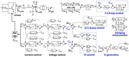
Figure 1.
Physical structure of a grid-forming converter and its control loops.
2.1.1. Modelling the Grid-Forming Converter Control Loops
The equations for active power and frequency, , droop control are given as (1)–(4), which model the active power injected by the converter, the measure of this power, the droop control, and the angle of the converter, respectively.
where is the rotating frequency of the common DQ0 reference frame.
The equations for reactive power and voltage amplitude (), droop control, along with a damping enhancement control and virtual impedance (VI)-based current-limiting control (the principle of the VI current-limiting control is that an emulated impedance is added to the filter once the converter’s current is larger than , so that the converter’s current is limited), are given as (5)–(15). Equations (5) and (6) model the reactive power injected by the converter and the measure of this power, (7) and (8) model the reactive droop control, (9) and (10) model the damping enhancement control, (11)–(14) model the VI current control, and (15) calculates the converter’s current.
The equations for the proportional integral (PI) control loop of the output voltage across the capacitor are given as (16)–(19), where (16) and (17) represent the integrator and (18) and (19) create the current reference for the inner current control loop.
Finally, the equations for the PI control loop of the converter current through the filter are given as (20)–(23), where (20) and (21) represent the integrator and (22) and (23) create the voltage reference of the DC/AC converter.
2.1.2. Modelling the Grid-Forming Converter Physical Hardware
The Equations (24)–(29) represent the RL filter (24) and (25), the C filter (26) and (27), and the DC/AC converter (28) and (29), based upon a DQ0 reference frame of the angular frequency given by the external loop.
Equations (28) and (29) indicate that the DC/AC converter is assumed to be ideal.
The output voltage and current in (24)–(27) need to be converted to the common DQ0 reference frame rotating at a frequency of , with a base capacity of 100 MVA. Given a converter capacity of , the conversions are presented as follows.
2.2. Transformers
The RL transformer is represented in Figure 2a and given in (32)–(35). These equations are given in pu, and in the common DQ0 reference frame of a frequency and base capacity of 100 MVA. A change in the transformer ratio is incorporated.
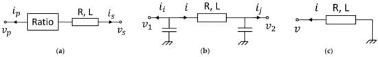
Figure 2.
(a) Transformer model, (b) Pi-line model, and (c) RL-load model.
2.3. Branches
It is assumed here that transmission lines are modelled as pi-models with a common DQ0 reference frame at frequency . The pi-line model is shown in Figure 2b with the equations summarised as (36)–(38), where (36) models the RL line, and (37) and (38) account the capacitive effects of the line.
2.4. Loads
The loads are represented here as RL-loads, as shown in Figure 2c, with the dynamic Equations (39) and (40) given in , and in the DQ0 reference frame at frequency .
3. Model Order Reduction by Combination of the State Residualisation and Kron Reduction Technique
3.1. State Residualisation Technique
3.1.1. State Residualisation Principle
A power system can be modelled as a nonlinear differential-algebraic system of equations (DAE) as (41).
where , , and represent the algebraic input and output variables, and , , and are the related orders.
The residualisation of a state variable consists of changing the state variable into an algebraic variable by neglecting its derivative in the associated differential equation, transforming it into an algebraic equation [9]. It represents a well-known process applied in the phasor approximation to state variables modelling power lines, and is used by most transient simulation programs [30].
The reduced system obtained by state residualisation can be written as in (42).
The diagonal matrix is called the residualisation matrix, consisting of or on its diagonal. Each diagonal element indicates whether the state variable is residualised or not. If , the state variable is residualised, and otherwise . The size of the reduced system is given by .
The objective of state residualisation is to choose , providing a trade-off between the order of the reduced model and the expected modelling error.
It is seen that the variables and parameters of the full and reduced models are exactly the same, which ensures that the steady state values of the full and reduced models are the same, as they are computed with the same system. It is also straightforward to directly consider the reduced system for analysis, or tuning and designing of controllers. Finally, state residualisation can be implemented in classical DAE solvers, as it involves substituting some derivative terms by 0.
A method to achieve state residualisation, consisting of state categorisation and modal state residualisation, as proposed by [25], is summarised in Figure 3.
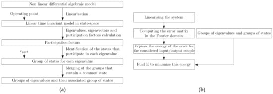
Figure 3.
(a) Synoptic describing the state categorisation [25], and (b) synoptic describing the modal state residualisation [25].
3.1.2. State Categorisation
Adopting the state residualisation method proposed by [25], the residualisation of state variables for a nonlinear model is linked to discarding some poles in the linearised model around its operating point and preserving the other poles. By acknowledging links between the states and poles of a linearised system, it is possible to choose which states to residualise in the nonlinear system. This process, illustrated in Figure 3a, is described step by step in the following.
- (1)
- Linearisation. The non-linear DAE model in (20) is linearised around a steady-state operating point [30], resulting in a linear time invariant system that can be represented in state space as in (43).
- (2)
- Participation Factor. Participation factors are a linear algebraic tool, introduced in [31], which quantify the links between the eigenvalues of a linear system and its state variables. More precisely, the participation factor is a complex number whose modulus gives the participation of the state in the eigenvalue (and vice versa) and indicates how much the state variable influences the considered pole. The participation factor is calculated as in (44):
The left and right eigenvectors of A should be normalised, such that the sum of all the participation factors of all states for an eigenvalue is equal to 1 (for example, , associated with eigenvalue ). Subsequently, the degree of participation of each state to an eigenvalue can be compared.
- (3)
- Groups of States and Eigenvalues. With obtained, the states that participate the most in each eigenvalue can be grouped together, with the rest discarded. Thus, groups (states that do not belong to any group can be set to zero, as they do not significantly contribute to any eigenvalue) are obtained, as there are eigenvalues. This process can be achieved by ordering in descending order and summing the first terms larger than a threshold, .
In a coupled system, a state variable may participate in several eigenvalues, which means that some of the previously created groups can be merged to form new groups, where each new group is associated with one or more eigenvalues. After this process, fewer than groups are normally left. The state variables in the same group can be residualised together, or not at all (using an optimisation method describe in the next subsection). In other words, the associated poles will be discarded together, or not.
Based on the above approach, the criterion indicates the precision of the state categorisation. If is high, interactions between the states are well recognised, but since the number of groups is reduced, the possibilities for reductions are limited. Alternatively, if is low, the reduction possibilities are improved but the precision with which the poles are retained will be poor. The choice of this criterion is empirical, but different values can easily be tested. This paper demonstrated that the choice of can be based on the type of event.
3.1.3. Modal State Residualisation
The developed state residualisation in [25] is based on finding which minimises an error criterion while respecting the state categorisation deduced in the previous subsection. It is a modal state residualisation, as the residualisation preserves some poles of the linearised system.
The error criterion to minimise is chosen to be , the square of the norm of the difference between the th output of the full model and the reduced model, excited by the th input with a Dirac function for a chosen norm. This choice is motivated by the objective of tracking the transient of some sensitive variables, such as the output current of some converters, for a specific simulated event, modelled here by input .
Since it can be complicated to calculate this error criterion for nonlinear models, both systems are linearised. For the full model, (43) is obtained, and for the reduced model, (46) is obtained.
It is also difficult to calculate the error criterion in the time domain. Hence, the error is calculated in the frequency domain. Based on (43)–(46), the transfer functions from the chosen input to output can be obtained as (47) and (48).
The difference between the two transfer functions gives (49).
The difference in the Fourier domain between the th output of the full model and of the reduced model when simulating a Dirac function for input is given by , where represents the element in the th row and th column. The energy of the error, , is defined in (50).
By minimising the energy, , the optimisation problem can be presented as in (51).
where represents that the states in the same group must be residualised (or not) together to discard (or keep), and is the desired size of the reduced model. In reference [25], is chosen arbitrarily, but here a systematic way is applied for choosing the order, so it is the same as the phasor approximation. The results in Section 4 will demonstrate that the reduced model leads to improved model accuracy.
A genetic algorithm [32]-based approach is used here to solve the optimisation problem (51), which allows a low computation time compared to bruteforce methods [33] (which involves listing all possible matrices, calculating the error , and choosing which minimises all ).
The modal state residualisation process is summarised in Figure 3b, where it is seen that the obtained is specific to the chosen output-input couple (). In other words, the obtained reduced models can be different for each considered test case: observed variables-output/simulated event-input. It follows that the method is flexible and can be adapted to any considered events and concerned variables (e.g., converter current).
3.2. The Kron Reduction Technique
After the above process, sections of the network are modelled as algebraic equations. Kron reduction can then be used to eliminate the passive nodes (i.e., no current injected). A passive node in the node admittance matrix can be eliminated by replacing the elements of the remaining rows and columns by
for and , where is the mutual admittance between nodes and (negative value of the sum of all admittances connected between nodes and ), and is the self admittance of node (sum of all admittances connected at node ).
By the successive application of (52), any desired number of passive nodes can be eliminated. Equation (52) is called Kron’s reduction formula, with further details of the method to be found in [34].
It is seen that after a Kron reduction process, fewer bus nodes and algebraic states/equations remain in a DAE model, such that the simulation time is reduced, which is particularly useful for power systems, where the number of passive bus nodes is much larger than the number of generation nodes.
4. Application and Results
4.1. General Structure of Modified IEEE 39-Bus System
The IEEE 10-generator, a 39-bus system [35] with 10 synchronous generators replaced by grid-forming converters, is considered, as shown in Figure 4a. Each GFM is modelled based on its defined base values, and . For the grid, , while is the same across the system. All equations for the electrical components are described in Section 2. The physical and control parameters of the GFMs are the same as in [4,29], as shown in Table 1, while the remaining parameters are the same as in [35]. Note that the maximum current for the GFMs is tuned to be 1.2 pu, by incorporating virtual impedance current-limiting control.
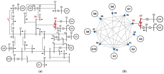
Figure 4.
(a) IEEE 39-bus system with the 10 synchronous generators replaced by grid-forming converters. (b) schematic diagram of reduced model after implementing state residualisation and Kron reduction technique for Cases 1 and 2, with the fault applied at bus 19.

Table 1.
Grid-forming converter RLC filter and control parameters.
Two short-circuits and one line-tripping event are simulated, and the state residualisation method is applied to the system in each case. The short-circuit is modelled as a shunt resistance, which switches from a very large to a very small value when the event is triggered. The resistance that creates the short-circuit is considered as the input for calculating the residualisation matrix in (42). Similarly, the line-tripping event is modelled by a series connected resistance that becomes very large when the event happens, with the resistance again considered as the residualisation matrix.
In order to demonstrate that the proposed technique achieves more accurate transient simulations than the traditional phasor approximate model, along with reducing the simulation time, the following cases are created:
Case 1: A bolted three-phase short-circuit is applied at bus 19 at 1 s, and cleared at 1.15 s.
Case 2: The same as Case 1, but the short-circuit is 10 times less severe, and the length (and series and shunt impedance) of line B16–19 is increased by a factor of 18 (a sufficiently large scaling that ensures that the system remains stable for different events and disturbances), so as to focus the impact on generators G4 and G5.
Case 3: Line B26–29 is disconnected at 1 s. In order to create a noticeable impact on the nearby generators, B26–29 is shortened by a factor of 10, while line B28–29 is lengthened by a factor of 10.
Different from [25], where only one converter is observed, the currents of all converters in the system are observed as outputs, as part of determining the residualisation matrix in (42), noting that the location of an event is not known a priori. Since the system topologies are different under the three events, the state residualisation needs to be determined separately in each case.
Here, the converter currents are chosen as the observed output variables, since (1) converters have a much lower overcurrent capability relative to synchronous machines, and (2) converter fast transient currents need to be captured with good accuracy to ensure converter integrity.
4.2. Application of State Residualisation Technique
The state categorisation described in Section 3.1.2 is applied to the three test cases, with selected as 0.75 for the short-circuit events in Cases 1 and 2, and 0.55 for the line-tripping event in Case 3, which results in three different grouping formulas, as shown in Table 2. The principle for choosing is not overly critical, but it should be based on the severity of an event, such that the less severe the event in question, the smaller should be, since for a less-severe event the states will be more likely to have equal participation in a mode. Hence, choosing a smaller for a less-severe event can disjoint the system states and separate them into different groups. In this way, the state variables that are most relevant to an event are grouped into individual groups, while the remainder are grouped into a few larger groups. In general, simply choosing as 0.75 for short-circuits, and as 0.55 for line-tripping, leads to satisfactory grouping.
Table 2.
Different groups are formed for different cases, given the topology changes.
Subsequently, modal state residualisation of (42) in Section 3.1.3 is applied, by choosing the desired size as equal to the phasor approximate model. Three reduced models are obtained, which are summarised in Table 3. For example, for Case 1, the variables to be retained are almost the same as for Case 2, except for the remaining GFMs, which are less impacted by the short-circuit. The result is not surprising given that the short-circuit is applied at the same bus, and the topology of each system is very similar. However, for Case 3, as the system topology is more noticeably different from the previous two cases, the variables to be retained are different.
Table 3.
Optimal reduced-order model obtained by using state residualisation for the different events.
It is seen that state residualisation helps to identify zones to reduce, while high-level details are retained elsewhere, depending on the simulated event. It is confirmed that those parts of the system that are located far from the simulated event are generally modelled with fewer details than those parts that are located nearby.
4.3. Dynamic Simulation Results and Analysis
For each case, three mode types are compared using time domain simulations: full order EMT model (order 308), phasor model (order 130, with the network modelled as algebraic equations), and reduced-order models based on the state residualisation results summarised in Table 3.
The simulations are performed using the Modelica [36] language as implemented using Dymola 2022 software. Modelica is very convenient when simulating DAE systems and for state residualisation, as the model equations are directly written. A variable integration time step is applied, such that a larger step size can be used when state variables representing fast dynamics are residualised (i.e., turned into algebraic variables). The integration tolerance is set as 0.0001.
For Cases 1–3, comparison simulation results of the 10 GFM currents are shown in Figure 5, Figure 6 and Figure 7, respectively, noting that a different reduced model should be used for each simulated event. Figure 5, Figure 6 and Figure 7 show that by choosing the model order to be the same as the phasor approximate model, that the reduced models better capture the GFM transients (as they retain the most relevant dynamics) over the RMS models. More precisely, the reduced models accurately simulate the GFMs that are the most impacted by the short-circuit and line-tripping events, i.e., G4 and G5 for Cases 1 and 2, and G9 for Case 3, while the phasor models miss the initial current peaks, and so would suggest that the converter current was within acceptable limits, when, in fact, it was not. For the other GFMs in Cases 1 and 2, the reduced models also capture the transients of the first peak current of the converters with better accuracy than the phasor approximated models, except G6 in Case 1 where the first peak current of G6 is slightly lower than with the phasor model. It is seen that the former correctly predict the trends of the first oscillation of the converter’s current with much smaller first peak errors, while the latter sometimes gives opposite directions for the first oscillations (for example for G1, G8 and G9 in Case 1) and tends to have a larger error for the first peak (e.g., the error is 0.1~0.3 pu for G2, G3, G7, and G10 in Case 1). Similarly, in Case 3, for the other GFMs, i.e., not G9, the low-frequency current oscillations in the full EMT model are better matched by the reduced model over the phasor model, although they both miss the first peaks, as seen in Figure 7, where in the phasor model the phases of the low-frequency oscillations are almost opposite to those in the full EMT model.
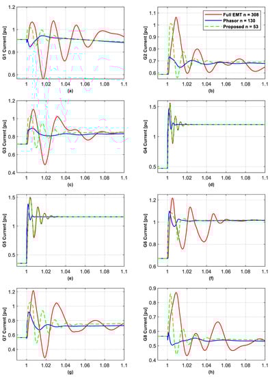
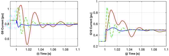
Figure 5.
Converter current for GFMs located at buses 30–39 for the full EMT, phasor, and proposed reduced model for a 150 ms short-circuit applied at bus 19 at 1 s under Case 1. (a–j) the current of the GFMs at bus 39 and 30–38, respectively, as shown in Figure 4.
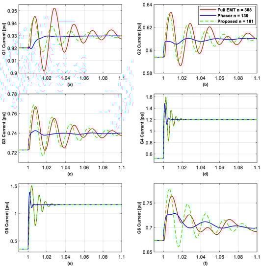
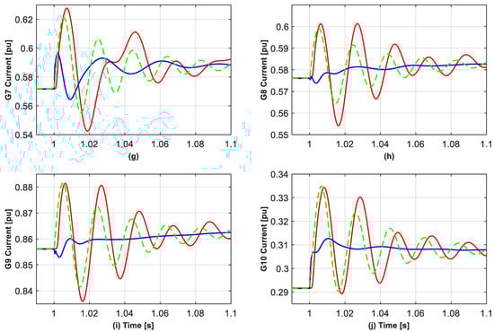
Figure 6.
Converter current for GFMs located at buses 30–39 for the full EMT, phasor, and proposed reduced model for a 150 ms short-circuit applied at bus 19 at 1 s under Case 2. (a–j) the current of the GFMs at bus 39 and 30–38, respectively, as shown in Figure 4.
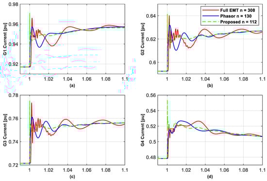
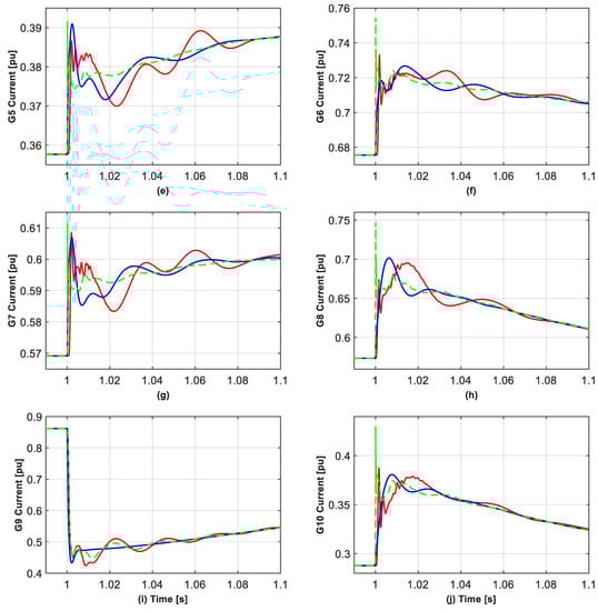
Figure 7.
Converter current for GFM located at buses 30–39 for the full EMT, phasor, and proposed reduced model when tripping line B26–29 at 1 s under Case 3. (a–j) the current of the GFMs at bus 39 and 30–38, respectively, as shown in Figure 4.
It is also seen that for other GFMs in Cases 1–3, the reduced models tend to give a faster initial current rise (which is also seen in the phasor models) and tend to slightly underestimate or overestimate the maximum current, which is, however, not critical for respecting converter integrity. The reason for this is because the dynamics of a large part of the network and the filter of the less-impacted converters are not modelled.
Note that in Cases 1 and 2, the current of G4, and also G5, is greater than the 1.2 pu limit, which is due to the “soft” virtual impedance-based current-limiting control, which cannot strictly limit the converter current.
Table 4 shows the average absolute error of the peak/valley for the first oscillation cycle of the current for the 10 GFMs relative to the equivalent oscillation for the full EMT model from 1.00~1.01 s for the phasor and state residualisation approaches for Cases 1–3. It is seen for the severe fault in Case 1 that the average error in the phasor model is 3.8 times greater than that for the reduced model; for the less-severe fault in Case 2, the average error for the phasor model is 14.9 times worse than the reduced model; while for line disconnection event in Case 3, the phasor model actually performs better than the reduced model, although both models can be used for Case 3, since Figure 7 shows that the current of the most relevant converter, G9, is accurately represented in both models (although the reduced model performs a little better with more accurate capture of the timing of the current drop and waveforms of the current oscillations), and other generators with small impact are also reasonably represented.
Table 4.
Average absolute error for the first current oscillation cycle for the 10 GFMs relative to the equivalent for the full EMT model over 1~1.01 s for the phasor and state residualisation approaches for Cases 1–3.
Figure 8, Figure 9 and Figure 10 compare the poles of the linearised EMT, phasor, and reduced model of the faulted systems for Cases 1–3, respectively. The linearised A matrix is obtained by using the Linearize tool in Dymola software, which performs a linearisation based on the real-time operating point at a specific time point. The time point is set immediately after an event is applied, and hence the impact of the simulation event as an input can be captured in the linearised model. Note that the aim of presenting Figure 8, Figure 9 and Figure 10 is not to conduct detailed small-signal analysis but to show the match degree of the reduced and phasor models to the full EMT model.
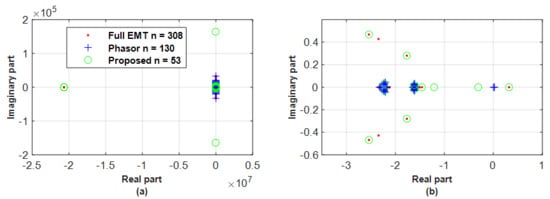
Figure 8.
(a) Poles of linearised full EMT, phasor, and proposed reduced model, for a 150 ms short-circuit applied at bus 19 at 1 s under Case 1, and (b) zoomed figure.
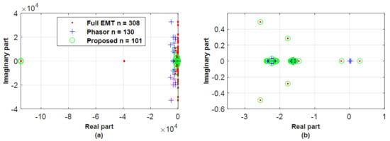
Figure 9.
(a) Poles of linearised full EMT, phasor, and proposed reduced model, for a 150 ms short-circuit applied at bus 16 at 1 s under Case 2, and (b) zoomed figure.
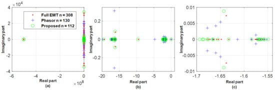
Figure 10.
(a) Poles of linearised full EMT, phasor, and proposed reduced model, for tripping line B26–29 at 1 s under Case 3, (b) and (c) zoomed figure.
Figure 8 and Figure 9 show that the critical poles (i.e., rightmost poles that dominate the system transients) of the reduced models are well overlapped with those of the full EMT model, while the phasor models fail to represent the unstable poles 0.3 (participation factor calculations show that the two unstable poles are mainly contributed by and of G3 and G4 (95%)) and critical oscillation modes.
Figure 8 and Figure 9 also show that the state residualisation reduced model in Case 2 appears to better preserve the critical poles over Case 1, as in Case 1 the pole pair is not matched and extra poles −0.3 and −1.15 are added, which is also reflected in the time simulation results in Figure 5 and Figure 6.
Figure 10 shows that both (state residualisation and phasor) reduced models miss some critical poles, e.g., and as seen in Figure 10c. However, these dominant poles are seen to be very close with each other (within a 0.01 distance difference) and hence both models can be used, which is also confirmed by the time domain results in Figure 7 as the current of G9 with the severest impact is accurately represented in both models.
Figure 8a, Figure 9a, and Figure 10a all show that the reduced model keeps the most-left poles, which, however, failed in the phasor model. It, with the above results of preserving critical poles and adding some extra pole, thus illustrates that the reduced model is able to keep the more energetic poles, through achieving the target, (51), of minimising the energy error for each the simulated event input to the observed variables output.
Three main conclusions can be drawn from the above dynamic simulation results. Firstly, the most appropriate reduced model depends on the location and nature of the simulated event. Secondly, by making the model order the same, state residualisation can capture event transients with better accuracy than phasor approximation models, particularly for short-circuit events where converter overcurrents are of most concern. Finally, for short-circuits, the phasor approximation model does not achieve good accuracy, and it is particularly concerning that the fast initial transients (very important for power converters) may be missed.
4.4. Application of Kron Reduction Technique
After applying state residualisaton, the classic Kron reduction technique [34] can be implemented to further reduce network complexity, and, subsequently, the simulation time. For illustration, a schematic diagram of the reduced model for Cases 1 and 2 for a fault applied at bus 19 is shown in Figure 4b. It is seen that the number of bus nodes is reduced from 39 to 13. Moreover, the voltage and current relationships of the Kron reduced network are represented by an algebraic matrix, which simplifies subsequent implementation.
Table 5 compares the simulation time of the reduced models by using the proposed and phasor approximation technique under Cases 1–3. It is seen that both the reduced models, based on phasor approximation and the proposed combination of state residualisation and Kron reduction, require less execution time than the full EMT models (i.e., 20~80%, depending on the test scenario), with the latter being faster than the former (15~20% reduction achieved). It is also seen that the reduction in simulation time, relative to the full EMT model, is different under the three cases, which is, as expected, given the nature of the disturbance event and its proximity to nearby generators.
Table 5.
Simulation time of reduced models, using state residualisation and Kron reduction compared to phasor models (order 130), relative to full EMT models (order 308).
5. Conclusions
A combination of event- and non-projection state residualisation approximation and Kron reduction techniques has been presented, which maintains the advantages of both approaches. The former preserves the variables and physical structure of a system by using state residualisation instead of projections, retains some poles around the operating point (ensuring stability preservation), and adapts to the simulated event and observed variables. The latter simplifies the network representation of the obtained models, and thus further speeds up the time domain simulation. This method has been applied to a modified IEEE 39-bus system with 100% PE converters under different test cases. The results show that selecting the reduced model size to be the same as the phasor approximation reduces model complexity while achieving improved accuracy and faster simulation times. The main reason for the improvements seen is that the state residualisation method adapts to the test case under consideration and thus achieves the most appropriate reduced model, while the Kron reduction reduces the number of bus nodes required.
Author Contributions
Conceptualisation, methodology and resources, X.Z. and X.K.; software, validation, formal analysis, investigation, data curation and writing—original draft preparation, X.Z.; writing—review and editing, X.Z., X.K., Q.C., F.C. and D.F. All authors have read and agreed to the published version of the manuscript.
Funding
The work has been supported by SEAI (Sustainable Energy Authority of Ireland) under RD&D Award 22/RDD/776. It has also been supported by a Ulysses award from the Irish Research Council between UCD and L2EP, ENSAM.
Institutional Review Board Statement
Not applicable.
Informed Consent Statement
Not applicable.
Data Availability Statement
Data is currently unavailable due to privacy restrictions.
Conflicts of Interest
The authors declare no conflict of interest.
Nomenclature
The following variables are associated with the grid-forming converter (GFM) implemented in this paper.
| The injected, and measured active power | |
| The virtual angular speed and angle generated by the droop control | |
| The injected and measured reactive power | |
| The d- and q-axis voltage references for the inner voltage proportional-integral (PI) controller | |
| The d- and q-axis voltage across the filter | |
| The d- and q-axis current references for the inner current PI controller | |
| The d- and q-axis current through the filter | |
| The current amplitude through the filter | |
| The d- and q-axis states for the integrator of the voltage and current PI controllers | |
| The d- and q-axis voltage reference and real values of the DC/AC converter | |
| The d- and q-axis states for the damping enhancement control | |
| The generated d- and q-axis voltage of the damping enhancement control which are added to the outer loop voltage reference | |
| The generated d- and q-axis voltage of the virtual impedance current-limiting control which are added to the outer loop voltage reference | |
| The generated virtual impedance resistor and reactance |
References
- Hatziargyriou, N.; Milanović, J.; Rahmann, C.; Ajjarapu, V.; Cañizares, C.; Erlich, I.; Hill, D.; Hiskens, I.; Kamwa, I.; Pal, B. Stability Definitions and Characterization of Dynamic Behavior in Systems with High Penetration of Power Electronic Interfaced Technologies; IEEE PES Technical Report PES-TR77; IEEE: Piscataway, NJ, USA, 2020. [Google Scholar]
- Rocabert, J.; Luna, A.; Blaabjerg, F.; Rodriguez, P. Control of power converters in AC microgrids. IEEE Trans. Power Electron. 2012, 27, 4734–4749. [Google Scholar] [CrossRef]
- Yu, M.; Roscoe, A.J.; Dyśko, A.; Booth, C.D.; Ierna, R.; Zhu, J.; Urdal, H. Instantaneous penetration level limits of non-synchronous devices in the British power system. IET Renew. Power Gener. 2017, 11, 1211–1217. [Google Scholar] [CrossRef]
- Zhao, X.; Thakurta, P.G.; Flynn, D. Grid-forming requirements based on stability assessment for 100% converter-based Irish power system. IET Renew. Power Gener. 2022, 16, 447–458. [Google Scholar] [CrossRef]
- Markovic, U.; Stanojev, O.; Aristidou, P.; Vrettos, E.; Callaway, D.; Hug, G. Understanding small-signal stability of low-inertia systems. IEEE Trans. Power Syst. 2021, 36, 3997–4017. [Google Scholar] [CrossRef]
- De Siqueira, J.C.G.; Bonatto, B.D.; Marti, J.R.; Hollman, J.A.; Dommel, H.W. A discussion about optimum time step size and maximum simulation time in EMTP-based programs. Int. J. Electr. Power Energy Syst. 2015, 72, 24–32. [Google Scholar] [CrossRef]
- Vorobev, P.; Huang, P.H.; Al Hosani, M.; Kirtley, J.L.; Turitsyn, K. High-fidelity model order reduction for microgrids stability assessment. IEEE Trans. Power Syst. 2017, 33, 874–887. [Google Scholar] [CrossRef]
- Gu, Y.; Bottrell, N.; Green, T.C. Reduced-order models for representing converters in power system studies. IEEE Trans. Power Electron. 2017, 33, 3644–3654. [Google Scholar] [CrossRef]
- Antoulas, A.C. Approximation of Large-Scale Dynamical Systems; SIAM: Philadelphia, PA, USA, 2005. [Google Scholar]
- Varga, A. Enhanced modal approach for model reduction. Math. Model. Syst. 1995, 1, 91–105. [Google Scholar] [CrossRef]
- Zhou, J.; Shi, P.; Gan, D.; Xu, Y.; Xin, H.; Jiang, C.; Xie, H.; Wu, T. Large-scale power system robust stability analysis based on value set approach. IEEE Trans. Power Syst. 2017, 32, 4012–4023. [Google Scholar] [CrossRef]
- Marinescu, B.; Mallem, B.; Rouco, L. Large-scale power system dynamic equivalents based on standard and border synchrony. IEEE Trans. Power Syst. 2010, 25, 1873–1882. [Google Scholar] [CrossRef]
- Campos, N.d.M.D.; Sarnet, T.; Kilter, J. Novel Gramian-based Structure-preserving Model Order Reduction for Power Systems with High Penetration of Power Converters. IEEE Trans. Power Syst. 2022. [Google Scholar] [CrossRef]
- Ghosh, S.; Isbeih, Y.J.; El Moursi, M.S.; El-Saadany, E.F. Cross-gramian model reduction approach for tuning power system stabilizers in large power networks. IEEE Trans. Power Syst. 2019, 35, 1911–1922. [Google Scholar] [CrossRef]
- Willcox, K.; Peraire, J. Balanced model reduction via the proper orthogonal decomposition. AIAA J. 2002, 40, 2323–2330. [Google Scholar] [CrossRef]
- Chinesta, F.; Ladeveze, P.; Cueto, E. A short review on model order reduction based on proper generalized decomposition. Arch. Comput. Methods Eng. 2011, 18, 395. [Google Scholar] [CrossRef]
- Chaniotis, D.; Pai, M. Model reduction in power systems using Krylov subspace methods. IEEE Trans. Power Syst. 2005, 20, 888–894. [Google Scholar] [CrossRef]
- Ali, H.R.; Pal, B.C. Model order reduction of multi-terminal direct-current grid systems. IEEE Trans. Power Syst. 2020, 36, 699–711. [Google Scholar] [CrossRef]
- Levron, Y.; Belikov, J. Reduction of power system dynamic models using sparse representations. IEEE Trans. Power Syst. 2017, 32, 3893–3900. [Google Scholar] [CrossRef]
- Grdenić, G.; Delimar, M.; Beerten, J. AC Grid Model Order Reduction Based on Interaction Modes Identification in Converter-Based Power Systems. IEEE Trans. Power Syst. 2022, 38, 2388–2397. [Google Scholar] [CrossRef]
- Scarciotti, G. Low computational complexity model reduction of power systems with preservation of physical characteristics. IEEE Trans. Power Syst. 2016, 32, 743–752. [Google Scholar] [CrossRef]
- Acle, Y.G.I.; Freitas, F.D.; Martins, N.; Rommes, J. Parameter preserving model order reduction of large sparse small-signal electromechanical stability power system models. IEEE Trans. Power Syst. 2019, 34, 2814–2824. [Google Scholar] [CrossRef]
- Ajala, O.; Baeckeland, N.; Johnson, B.; Dhople, S.; Domínguez-García, A. Model Reduction and Dynamic Aggregation of Grid-forming Inverter Networks. IEEE Trans. Power Syst. 2022. [Google Scholar] [CrossRef]
- Cossart, Q. Outils et Méthodes Pour L’analyse et la Simulation de Réseaux de Transport 100% Électronique de Puissance. Laboratoire d’Electrotechnique et d’Electronique de Puissance (L2EP) de Lille. Ph.D. Thesis, Hesam Université, Paris, France, 2019. [Google Scholar]
- Cossart, Q.; Colas, F.; Kestelyn, X. A Novel Event-and Non-Projection-Based Approximation Technique by State Residualization for the Model Order Reduction of Power Systems with a High Renewable Energies Penetration. IEEE Trans. Power Syst. 2020, 37, 3221–3229. [Google Scholar] [CrossRef]
- Pagola, F.L.; Perez-Arriaga, I.J.; Verghese, G.C. On sensitivities, residues and participations: Applications to oscillatory stability analysis and control. IEEE Trans. Power Syst. 1989, 4, 278–285. [Google Scholar] [CrossRef] [PubMed]
- Bottrell, N.; Green, T.C. Comparison of current-limiting strategies during fault ride-through of inverters to prevent latch-up and wind-up. IEEE Trans. Power Electron. 2013, 29, 3786–3797. [Google Scholar] [CrossRef]
- D’Arco, S.; Suul, J.A.; Fosso, O.B. Automatic tuning of cascaded controllers for power converters using eigenvalue parametric sensitivities. IEEE Trans. Ind. Appl. 2014, 51, 1743–1753. [Google Scholar] [CrossRef]
- Qoria, T.; Gruson, F.; Colas, F.; Guillaud, X.; Debry, M.-S.; Prevost, T. Tuning of cascaded controllers for robust grid-forming voltage source converter. In Proceedings of the Power Systems Computation Conference (PSCC), Dublin, Ireland, 11–15 June 2018; pp. 1–7. [Google Scholar]
- Kundur, P.S.; Malik, O.P. Power System Stability and Control; McGraw-Hill Education: New York, NY, USA, 1994. [Google Scholar]
- Pérez-Arriaga, I.J.; Verghese, G.C.; Schweppe, F.C. Selective modal analysis with applications to electric power systems, Part I: Heuristic introduction. IEEE Trans. Power Appar. Syst. 1982, PAS-101, 3117–3125. [Google Scholar] [CrossRef]
- Lee, K.Y.; El-Sharkawi, M.A. Modern Heuristic Optimization Techniques: Theory and Applications to Power Systems; John Wiley & Sons: Hoboken, NJ, USA, 2008; Volume 39. [Google Scholar]
- Cossart, Q.; Colas, F.; Kestelyn, X. A priori error estimation of the structure-preserving modal model reduction by state residualization of a grid forming converter for use in 100% power electronics transmission systems. In Proceedings of the 15th IET International Conference on AC and DC Power Transmission (ACDC 2019), Coventry, UK, 5–7 February 2019. [Google Scholar]
- Grainger, J.J. Power System Analysis; McGraw-Hill: New York, NY, USA, 1999. [Google Scholar]
- Pai, A. Energy Function Analysis for Power System Stability; Springer Science & Business Media: Berlin/Heidelberg, Germany, 1989. [Google Scholar]
- Fritzson, P. Principles of Object-Oriented Modeling and Simulation with Modelica 3.3: A Cyber-Physical Approach; John Wiley & Sons: Hoboken, NJ, USA, 2014. [Google Scholar]
Disclaimer/Publisher’s Note: The statements, opinions and data contained in all publications are solely those of the individual author(s) and contributor(s) and not of MDPI and/or the editor(s). MDPI and/or the editor(s) disclaim responsibility for any injury to people or property resulting from any ideas, methods, instructions or products referred to in the content. |
© 2023 by the authors. Licensee MDPI, Basel, Switzerland. This article is an open access article distributed under the terms and conditions of the Creative Commons Attribution (CC BY) license (https://creativecommons.org/licenses/by/4.0/).