


DA-FER: Domain Adaptive Facial Expression Recognition


Abstract
1. Introduction
2. Related Works
2.1. Small Sample Size Problem in the Field of Expression Recognition
2.2. Domain Adaptive Method for Facial Expression Recognition
3. Proposed Method
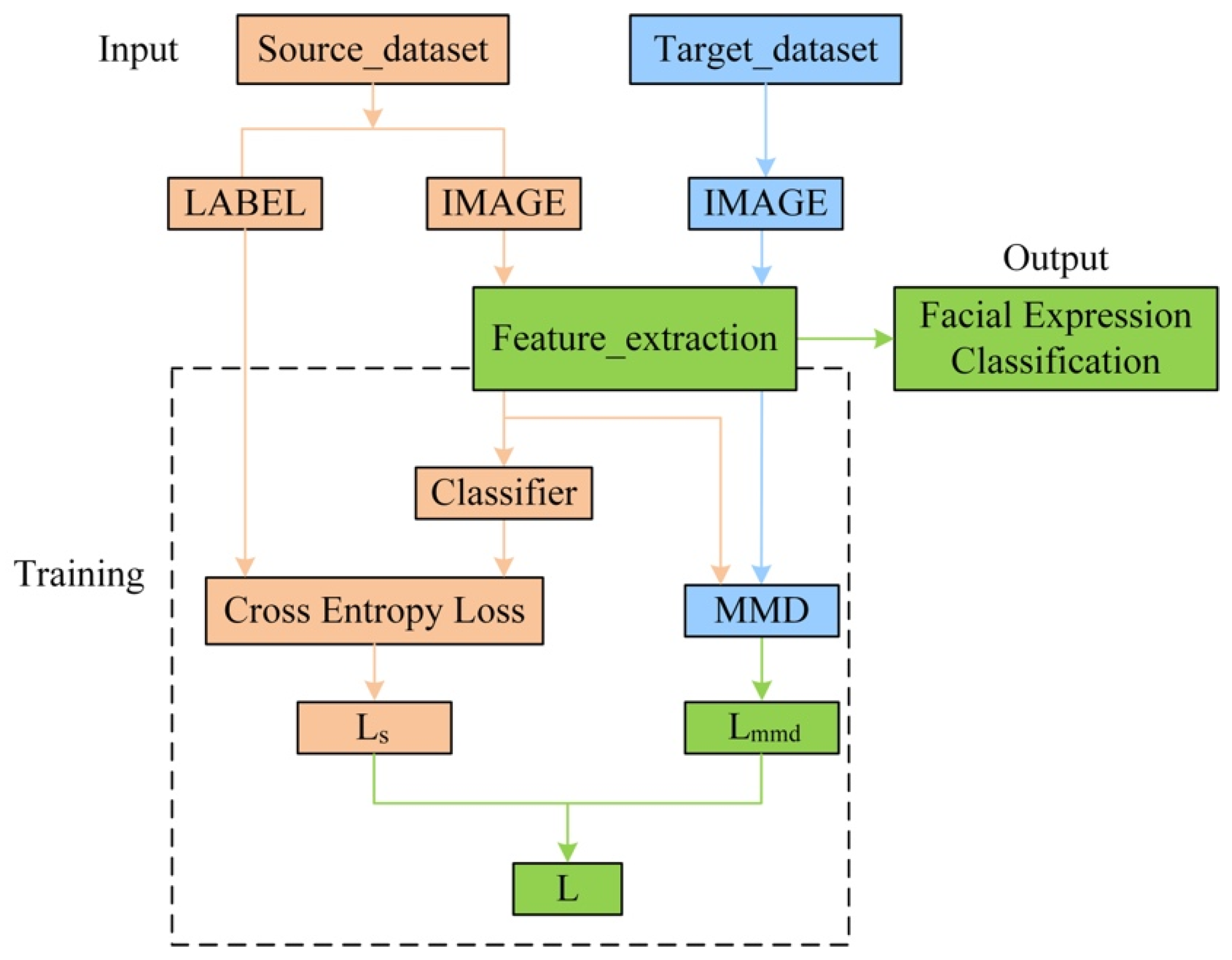
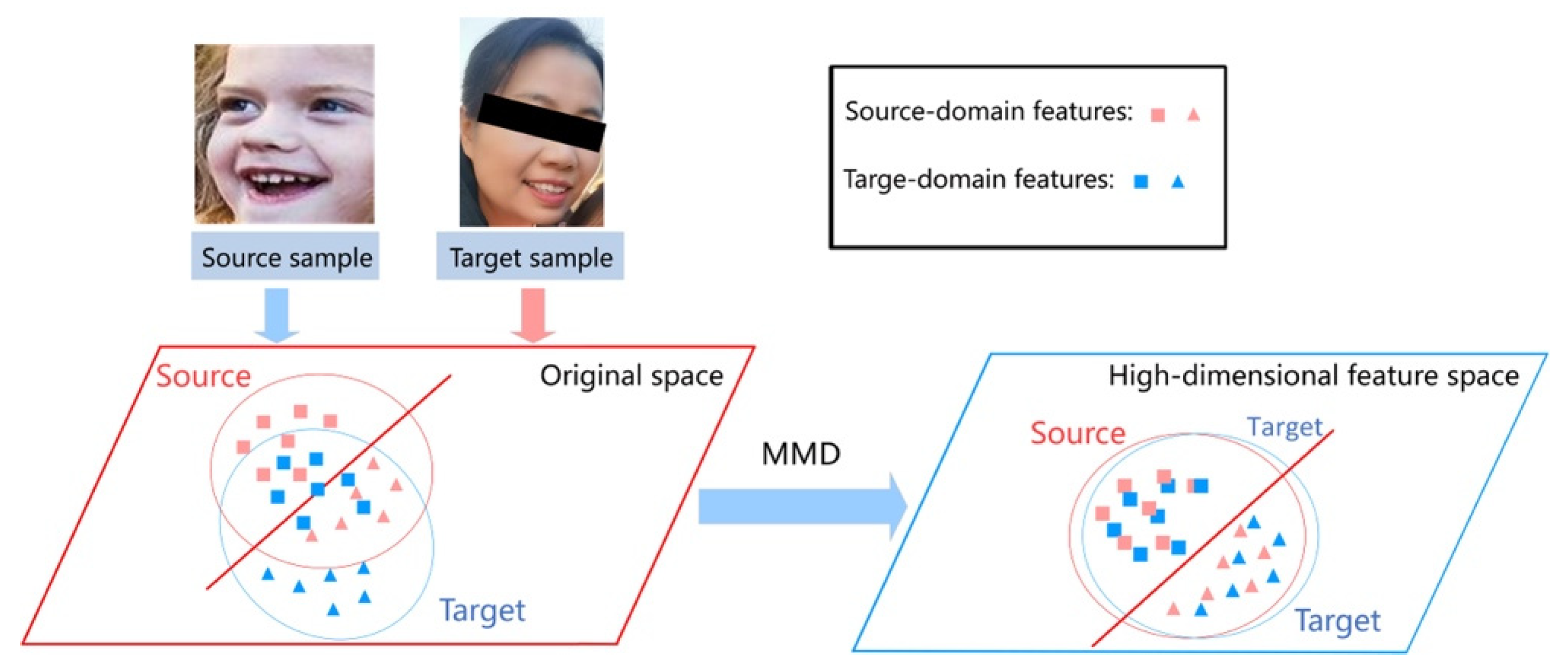
3.1. Learning Process of Domain Adaptive Method
3.2. Pre-Processing
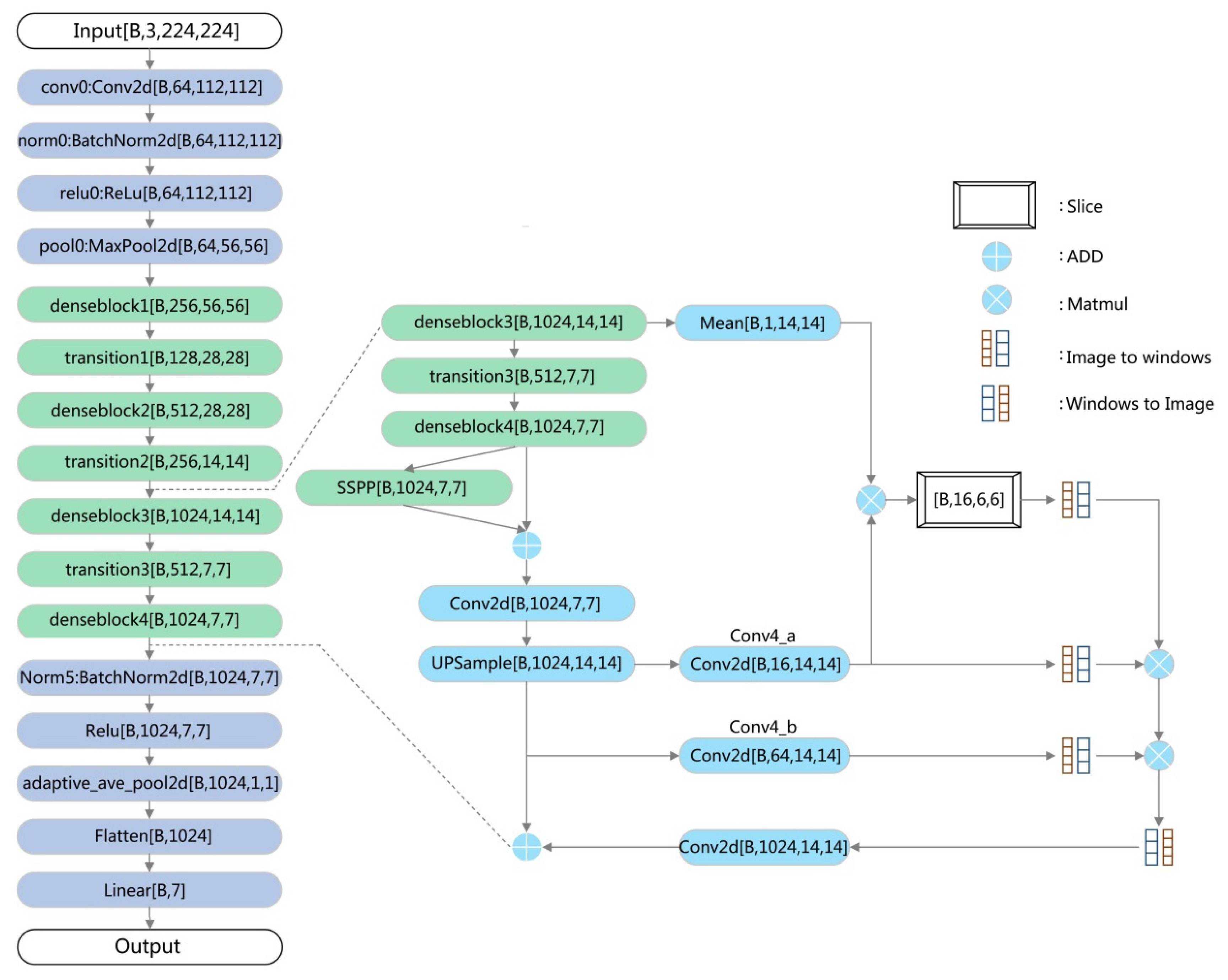
3.3. The Architecture of DA-FER
3.3.1. Mean
3.3.2. Small Space Pyramid Pooling
3.3.3. Slice Module
3.3.4. Adaptive Average Pooling
4. Experiment
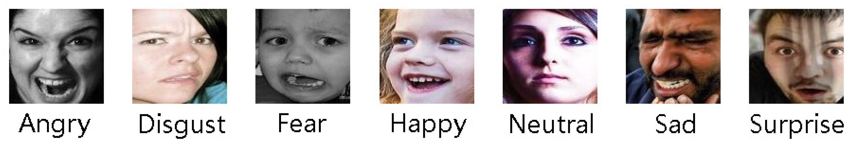
4.1. Dataset
4.1.1. Selfie-Expression as Target Domain
4.1.2. RAF-DB as Source Domain
4.1.3. Fer2013 as Source Domain
4.2. Experimental Environment
4.3. Results
5. Conclusions
Author Contributions
Funding
Institutional Review Board Statement
Informed Consent Statement
Data Availability Statement
Conflicts of Interest
References
- Li, Y.; Zhang, H.; Shen, Q. Spectral–spatial classification of hyperspectral imagery with 3D convolutional neural network. Remote Sens. 2017, 9, 67. [Google Scholar] [CrossRef]
- Wang, W.; Fu, Y.; Sun, Q.; Chen, T.; Cao, C.; Zheng, Z.; Xu, G.; Qiu, H.; Jiang, Y.G.; Xue, X. Learning to augment expressions for few-shot fine-grained facial expression recognition. arXiv 2020, arXiv:2001.06144. [Google Scholar]
- Shome, D.; Kar, T. FedAffect: Few-shot federated learning for facial expression recognition. In Proceedings of the IEEE/CVF International Conference on Computer Vision (ICCV), Electr Network, Montreal, QC, Canada, 11–17 October 2021; pp. 4168–4175. [Google Scholar] [CrossRef]
- Zhu, Q.; Mao, Q.; Jia, H.; Noi, O.E.N.; Tu, J. Convolutional relation network for facial expression recognition in the wild with few-shot learning. Expert Syst. Appl. 2022, 189, 116046. [Google Scholar] [CrossRef]
- Niu, S.; Liu, Y.; Wang, J.; Song, H. A decade survey of transfer learning (2010–2020). IEEE Trans. Artif. Intell. 2020, 1, 151–166. [Google Scholar] [CrossRef]
- Jin, C. Cross-database facial expression recognition based on hybrid improved unsupervised domain adaptation. Multimed. Tools Appl. 2023, 82, 1105–1129. [Google Scholar] [CrossRef]
- Álvarez-Pato, V.M.; Sánchez, C.N.; Domínguez-Soberanes, J.; Méndoza-Pérez, D.E.; Velázquez, R. A multisensor data fusion approach for predicting consumer acceptance of food products. Foods 2020, 9, 774. [Google Scholar] [CrossRef] [PubMed]
- Peng, X.; Gu, Y.; Zhang, P. Au-guided unsupervised domain-adaptive facial expression recognition. Appl. Sci. 2022, 12, 4366. [Google Scholar] [CrossRef]
- Kong, Y.S.; Suresh, V.; Soh, J.; Ong, D.C. A systematic evaluation of domain adaptation in facial expression recognition. arXiv 2021, arXiv:2106.15453. [Google Scholar]
- Xie, Y.; Gao, Y.; Lin, J.; Chen, T. Learning Consistent Global-Local Representation for Cross-Domain Facial Expression Recognition. In Proceedings of the 2022 26th International Conference on Pattern Recognition (ICPR), Montreal, QC, Canada, 21–25 August 2022; pp. 2489–2495. [Google Scholar] [CrossRef]
- Wu, Y.; Zhao, R.; Ma, H.; He, Q.; Du, S.; Wu, J. Adversarial domain adaptation convolutional neural network for intelligent recognition of bearing faults. Measurement 2022, 195, 111150. [Google Scholar] [CrossRef]
- Wang, T.; Ding, Z.; Shao, W.; Tang, H.; Huang, K. Towards fair cross-domain adaptation via generative learning. In Proceedings of the IEEE/CVF Winter Conference on Applications of Computer Vision (WACV), Electr Network, 5–9 January 2021; pp. 454–463. [Google Scholar] [CrossRef]
- Kang, G.; Jiang, L.; Yang, Y.; Hauptmann, A.G. Contrastive adaptation network for unsupervised domain adaptation. In Proceedings of the IEEE/CVF Conference on Computer Vision and Pattern Recognition, Long Beach, CA, USA, 15–20 June 2019; pp. 4893–4902. [Google Scholar] [CrossRef]
- Zhuang, F.; Qi, Z.; Duan, K.; Xi, D.; Zhu, Y.; Zhu, H.; Xiong, H.; He, Q. A comprehensive survey on transfer learning. Proc. IEEE 2020, 109, 43–76. [Google Scholar] [CrossRef]
- Shen, J.; Qu, Y.; Zhang, W.; Yu, Y. Wasserstein distance guided representation learning for domain adaptation. In Proceedings of the AAAI Conference on Artificial Intelligence, New Orleans, LA, USA, 2–7 February 2018; Volume 32. [Google Scholar] [CrossRef]
- Zhu, Y.; Zhuang, F.; Wang, J.; Xi, D.; Zhu, Y.; Zhu, H.; Xiong, H.; He, Q. Deep subdomain adaptation network for image classification. IEEE Trans. Neural Netw. Learn. Syst. 2020, 32, 1713–1722. [Google Scholar] [CrossRef] [PubMed]
- Yang, B.; Lei, Y.; Jia, F.; Li, N.; Du, Z. A polynomial kernel induced distance metric to improve deep transfer learning for fault diagnosis of machines. IEEE Trans. Ind. Electron. 2019, 67, 9747–9757. [Google Scholar] [CrossRef]
- Zhuang, J.; Jia, M.; Ding, Y.; Ding, P. Temporal convolution-based transferable cross-domain adaptation approach for remaining useful life estimation under variable failure behaviors. Reliab. Eng. Syst. Saf. 2021, 216, 107946. [Google Scholar] [CrossRef]
- Ding, R.; Li, X.; Nie, L.; Li, J.; Si, X.; Chu, D.; Liu, G.; Zhan, D. Empirical study and improvement on deep transfer learning for human activity recognition. Sensors 2018, 19, 57. [Google Scholar] [CrossRef] [PubMed]
- Chen, Z.; Wang, C.; Wu, J.; Deng, C.; Wang, Y. Deep convolutional transfer learning-based structural damage detection with domain adaptation. Appl. Intell. 2022, 53, 5085–5099. [Google Scholar] [CrossRef]
- Wu, X.; Ward, R.; Bottou, L. Wngrad: Learn the learning rate in gradient descent. arXiv 2018, arXiv:1803.02865. [Google Scholar]
- Takase, T.; Oyama, S.; Kurihara, M. Effective neural network training with adaptive learning rate based on training loss. Neural Netw. 2018, 101, 68–78. [Google Scholar] [CrossRef]
- Venkateswara, H.; Eusebio, J.; Chakraborty, S.; Panchanathan, S. Deep hashing network for unsupervised domain adaptation. In Proceedings of the IEEE Conference on Computer Vision and Pattern Recognition (CVPR), Honolulu, HI, USA, 21–26 July 2017; pp. 5018–5027. [Google Scholar] [CrossRef]
- Al-Khamees, H.A.A.A.; Al-A’araji, N.; Al-Shamery, E.S. Enhancing the stability of the deep neural network using a non-constant learning rate for data stream. Int. J. Electr. Comput. Eng. 2023, 13, 2123–2130. [Google Scholar] [CrossRef]
- Long, M.; Cao, Z.; Wang, J.; Jordan, M.I. Conditional adversarial domain adaptation. Adv. Neural Inf. Process. Syst. 2018, 31. [Google Scholar] [CrossRef]
- Pérez-García, F.; Sparks, R.; Ourselin, S. TorchIO: A Python library for efficient loading, preprocessing, augmentation and patch-based sampling of medical images in deep learning. Computer Methods Programs Biomed. 2021, 208, 106236. [Google Scholar] [CrossRef]
- Azizi, S.; Mustafa, B.; Ryan, F.; Beaver, Z.; Freyberg, J.; Deaton, J.; Loh, A.; Karthikesalingam, A.; Kornblith, S.; Chen, T.; et al. Big self-supervised models advance medical image classification. In Proceedings of the IEEE/CVF International Conference on Computer Vision (ICCV), Electr Network, Montreal, QC, Canada, 11–17 October 2021; pp. 3478–3488. [Google Scholar] [CrossRef]
- Hu, F.; Xia, G.S.; Hu, J.; Zhang, L. Transferring deep convolutional neural networks for the scene classification of high-resolution remote sensing imagery. Remote Sens. 2015, 7, 14680–14707. [Google Scholar] [CrossRef]
- Aghamaleki, J.A.; Ashkani Chenarlogh, V. Multi-stream CNN for facial expression recognition in limited training data. Multimed. Tools Appl. 2019, 78, 22861–22882. [Google Scholar] [CrossRef]
- Goodfellow, I.; Bengio, Y.; Courville, A. Deep Learning; MIT Press: Cambridge, UK, 2016. [Google Scholar] [CrossRef]
- Tan, X.; Triggs, B. Enhanced local texture feature sets for face recognition under difficult lighting conditions. IEEE Trans. Image Process. 2010, 19, 1635–1650. [Google Scholar] [CrossRef] [PubMed]
- James, G.; Witten, D.; Hastie, T.; Tibshirani, R. An Introduction to Statistical Learning; Springer: New York, NY, USA, 2013; Volume 112. [Google Scholar]
- He, K.; Zhang, X.; Ren, S.; Sun, J. Spatial pyramid pooling in deep convolutional networks for visual recognition. IEEE Trans. Pattern Anal. Mach. Intell. 2015, 37, 1904–1916. [Google Scholar] [CrossRef]
- Zheng, K.; Lan, C.; Zeng, W.; Zhang, Z.; Zha, Z.J. Exploiting sample uncertainty for domain adaptive person re-identification. In Proceedings of the AAAI Conference on Artificial Intelligence, Electr Network, 2–9 February 2021; Volume 35, pp. 3538–3546. [Google Scholar] [CrossRef]
- Alahmadi, A.; Hussain, M.; Aboalsamh, H.A.; Zuair, M. PCAPooL: Unsupervised feature learning for face recognition using PCA, LBP, and pyramid pooling. Pattern Anal. Appl. 2020, 23, 673–682. [Google Scholar] [CrossRef]
- Gu, Y.; Yan, H.; Zhang, X.; Liu, Z.; Ren, F.J. 3-d facial expression recognition via attention-based multichannel data fusion network. IEEE Trans. Instrum. Meas. 2021, 70, 3125972. [Google Scholar] [CrossRef]
- Bi, C.; Hu, N.; Zou, Y.; Zhang, S.; Xu, S.; Yu, H. Development of deep learning methodology for maize seed variety recognition based on improved swin transformer. Agronomy 2022, 12, 1843. [Google Scholar] [CrossRef]
- Donahue, J.; Jia, Y.; Vinyals, O.; Hoffman, J.; Zhang, N.; Tzeng, E.; Darrell, T. DeCAF: A deep convolutional activation feature for generic visual recognition. In Proceedings of the International Conference on Machine Learning, (CYCLE1), Beijing, China, 22–24 June 2014; Volume 32, pp. 647–655. [Google Scholar] [CrossRef]
- Shin, H.C.; Roth, H.R.; Gao, M.; Lu, L.; Xu, Z.; Nogues, I.; Yao, J.; Mollura, D.; Summers, R.M. Deep convolutional neural networks for computer-aided detection: CNN architectures, dataset characteristics and transfer learning. IEEE Trans. Med. Imaging 2016, 35, 1285–1298. [Google Scholar] [CrossRef]
- Ozcan, T.; Basturk, A. Static facial expression recognition using convolutional neural networks based on transfer learning and hyperparameter optimization. Multimed. Tools Appl. 2020, 79, 26587–26604. [Google Scholar] [CrossRef]
- Tzeng, E.; Hoffman, J.; Darrell, T.; Saenko, K. Simultaneous deep transfer across domains and tasks. In Proceedings of the IEEE Conference on Computer Vision and Pattern Recognition (ICCV), Santiago, Chile, 11–18 December 2015; pp. 4068–4076. [Google Scholar] [CrossRef]
- Li, S.; Deng, W.; Du, J.P. Reliable crowdsourcing and deep locality-preserving learning for expression recognition in the wild. In Proceedings of the IEEE Conference on Computer Vision and Pattern Recognition (CVPR), Honolulu, HI, USA, 21–26 July 2017; pp. 2852–2861. [Google Scholar] [CrossRef]
- Nguyen, D.; Sridharan, S.; Nguyen, D.T.; Denman, S.; Tran, S.N.; Zeng, R.; Fookes, C. Joint Deep Cross-Domain Transfer Learning for Emotion Recognition. arXiv 2020, arXiv:2003.11136. [Google Scholar]
- Chen, Y.; Joo, J. Understanding and mitigating annotation bias in facial expression recognition. In Proceedings of the IEEE/CVF International Conference on Computer Vision (ICCV), Electr Network, Montreal, QC, Canada, 11–17 October 2021; pp. 14980–14991. [Google Scholar] [CrossRef]
- Xue, F.; Wang, Q.; Guo, G. Transfer: Learning relation-aware facial expression representations with transformers. In Proceedings of the IEEE/CVF International Conference on Computer Vision (ICCV), Electr Network, Montreal, QC, Canada, 11–17 October 2021; pp. 3601–3610. [Google Scholar] [CrossRef]
- Li, H.; Wang, N.; Yang, X.; Wang, X.; Gao, X. Towards semi-supervised deep facial expression recognition with an adaptive confidence margin. In Proceedings of the IEEE/CVF Conference on Computer Vision and Pattern Recognition (CVPR), New Orleans, LA, USA, 18–24 June 2022; pp. 4166–4175. [Google Scholar] [CrossRef]
- Farzaneh, A.H.; Qi, X. Facial expression recognition in the wild via deep attentive center loss. In Proceedings of the IEEE/CVF Winter Conference on Applications of Computer Vision (WACV), Electr Network, Waikoloa, HI, USA, 5–9 January 2021; pp. 2402–2411. [Google Scholar] [CrossRef]


| Expression | Neutral | Happy | Surprise | Disgust | Fear | Sad | Anger | Total |
|---|---|---|---|---|---|---|---|---|
| Train | 114 | 105 | 83 | 81 | 81 | 71 | 71 | 606 |
| Test | 48 | 45 | 36 | 35 | 34 | 31 | 31 | 260 |
| Total | 162 | 150 | 119 | 116 | 115 | 102 | 102 | 866 |
| Expression | Happy | Neutral | Sad | Surprise | Disgust | Anger | Fear | Total |
|---|---|---|---|---|---|---|---|---|
| Train | 4772 | 2524 | 1982 | 1290 | 717 | 705 | 281 | 12,271 |
| Test | 1185 | 680 | 478 | 329 | 160 | 162 | 74 | 3068 |
| Total | 5957 | 3204 | 2460 | 1619 | 877 | 867 | 355 | 15,339 |
| Expression | Happy | Neutral | Sad | Fear | Anger | Surprise | Disgust | Total |
|---|---|---|---|---|---|---|---|---|
| Train | 7215 | 4965 | 4830 | 4097 | 3995 | 3171 | 436 | 28,709 |
| Test | 1774 | 1233 | 1247 | 1024 | 958 | 831 | 111 | 7178 |
| Total | 8989 | 6198 | 6077 | 5121 | 4953 | 4002 | 547 | 35,877 |
| Parameters Name | Parameters |
|---|---|
| Learning rate | 0.003 |
| Learning gamma | 0.0003 |
| Learning decay | 0.75 |
| Weight for mmd | 0.5 |
| Seed | 1024 |
| Total epoch | 100 |
| Batchsize | 64 |
| Mini_batchsize | 100/200 |
| Optimizer | SGD |
| Learning scheduler | Lambda |
| Network | Baseline- None | Baseline- True | Source- RAF-DB Mini_100 | Source- Fer2013 Mini_100 | Source- RAF-DB Mini_200 | Source- Fer2013 Mini_200 |
|---|---|---|---|---|---|---|
| AlexNet | 18.75 | 18.75 | 41.15 | 43.07 | 41.15 | 45.00 |
| DenseNet121 | 48.82 | 53.51 | 52.69 | 48.46 | 52.69 | 49.23 |
| Resnet-34 | 47.65 | 50.00 | 53.85 | 51.92 | 51.92 | 50.00 |
| Resnet-50 | 35.54 | 39.45 | 49.62 | 49.62 | 49.23 | 50.38 |
| VGG11 | 42.57 | 40.62 | 40 | 48.85 | 40.38 | 46.92 |
| VGG13 | 18.75 | 18.75 | 40.77 | 46.54 | 40.77 | 46.54 |
| VGG16 | 18.75 | 19.14 | 43.46 | 48.07 | 42.31 | 46.92 |
| DA-FER | - | - | 58.46 | 51.54 | 56.15 | 50.77 |
| Network | Baseline- None | Baseline- True | Source- RAF-DB Mini_100 | Source- Fer2013 Mini_100 | Source- RAF-DB Mini_200 | Source- Fer2013 Mini_200 |
|---|---|---|---|---|---|---|
| DenseNet121 | 0.63 | 0.66 | 0.77 | 0.69 | 0.71 | 0.73 |
| Resnet-34 | 0.66 | 0.64 | 0.76 | 0.73 | 0.77 | 0.70 |
| DA-FER | 0.76 | 0.76 | 0.80 | 0.76 |
| Feature Extraction Network | Number of Trainable Parameters | Number of Parameters | Inference Time Mini-100 |
|---|---|---|---|
| AlexNet | 4,831,047 | 4.83 M | 6.69 s |
| DenseNet121 | 19,800,967 | 19.8 M | 5 s |
| Resnet-34 | 21,417,799 | 21.42 M | 6.82 s |
| Resnet-50 | 24,034,375 | 24.03 M | 5 s |
| VGG11 | 15,645,063 | 15.65 M | 5 s |
| VGG13 | 15,829,575 | 15.83 M | 7.47 s |
| VGG16 | 21,139,271 | 21.14 M | 7.36 s |
| DA-FER | 9,365,415 | 9.37 M | 5s |
Disclaimer/Publisher’s Note: The statements, opinions and data contained in all publications are solely those of the individual author(s) and contributor(s) and not of MDPI and/or the editor(s). MDPI and/or the editor(s) disclaim responsibility for any injury to people or property resulting from any ideas, methods, instructions or products referred to in the content. |
© 2023 by the authors. Licensee MDPI, Basel, Switzerland. This article is an open access article distributed under the terms and conditions of the Creative Commons Attribution (CC BY) license (https://creativecommons.org/licenses/by/4.0/).
Share and Cite
Bie, M.; Xu, H.; Liu, Q.; Gao, Y.; Song, K.; Che, X. DA-FER: Domain Adaptive Facial Expression Recognition. Appl. Sci. 2023, 13, 6314. https://doi.org/10.3390/app13106314
Bie M, Xu H, Liu Q, Gao Y, Song K, Che X. DA-FER: Domain Adaptive Facial Expression Recognition. Applied Sciences. 2023; 13(10):6314. https://doi.org/10.3390/app13106314
Chicago/Turabian StyleBie, Mei, Huan Xu, Quanle Liu, Yan Gao, Kai Song, and Xiangjiu Che. 2023. "DA-FER: Domain Adaptive Facial Expression Recognition" Applied Sciences 13, no. 10: 6314. https://doi.org/10.3390/app13106314
APA StyleBie, M., Xu, H., Liu, Q., Gao, Y., Song, K., & Che, X. (2023). DA-FER: Domain Adaptive Facial Expression Recognition. Applied Sciences, 13(10), 6314. https://doi.org/10.3390/app13106314