Abstract
In order to reduce the sea clutter interference in the detection of sea surface targets, we propose a bistatic sea clutter suppression method based on compressed sensing optimization in this paper. The proposed method mitigates the interference effect by reconstructing and cancelling out the sea clutter. Since the fixed sparse base is not always completely applicable for the sparse representation of sea clutter, we propose a sparse base optimization algorithm based on transfer learning to convert the fixed sparse base into an adaptive one. Moreover, we introduce a sensing matrix optimization algorithm to decrease the cross-correlation coefficient between the measurement matrix and the sparse base matrix, which can enhance the signal reconstruction quality. Finally, we use the orthogonal matching pursuit algorithm to reconstruct the sea clutter and employ the reconstructed results to cancel and suppress the sea clutter. The simulation results demonstrate that the proposed method outperforms the traditional methods such as the root time-domain cancellation method and the singular value decomposition method (SVD). Therefore, the proposed method has great practical significance for the detection of bistatic sea surface targets.
1. Introduction
When detecting targets on the sea surface with radar, the existence of sea clutter presents great challenges to the detection task. Sea clutter refers to the backscattered echoes received by the radar from the sea surface, which comprises wind waves, gravity waves, and surface capillary waves, etc. In the sea target detection of bistatic radar, since the power of the sea clutter is much higher than the target echo, the target echo is usually submerged in the sea clutter, making it difficult for bistatic radar to accurately detect sea surface targets. Moreover, the existence of sea clutter will lead to false alarm or missing alarm in detection of sea surface targets. Therefore, it is very crucial to suppress sea clutter to achieve accurate detection of sea surface targets.
Currently, the traditional methods for sea clutter suppression can be broadly classified into three categories. The first category involves establishing models to fit the distribution of the sea clutter by studying the change characteristics of the sea clutter [1]. The second category is based on processing in the transform domain, including short-time Fourier transform (STFT), fractional Fourier transform (FRFT), wavelet transform (WT), etc. [2,3,4,5]. The third category is based on subspace decomposition theory, such as singular value decomposition (SVD) [6,7] and eigenvalue decomposition (EVD) [8]. However, the above methods have several disadvantages, including high computational requirements and limited application scenarios. Among these methods, the time-domain cyclic cancellation method (hereinafter referred to as root method) proposed by Root [9] is widely used in engineering due to its simple principle and low computational requirements. However, the root method’s parameter estimation error can result in an unstable clutter suppression effect.
On the other hand, the sparse representation theory inspires a new research idea for sea clutter suppression. For instance, Nguyen et al. proposed a sea clutter suppression method based on sparse optimization to separate the target echo from the sea clutter echo [10]. Similarly, Farshchian suggested a sea target extraction method based on sparse separation of sea clutter spectrum [11]. Rosenberg et al. explored three different formulas for sparse signal separation, utilizing short-time Fourier transform as a dictionary to separate stationary and moving targets from sea clutter with greater accuracy [12].
Against this background, this paper makes distinct contributions as follows: We consider the main factors affecting bistatic sea clutter for the scenario of bistatic sea surface target detection and analyze and model the bistatic sea clutter. The analysis results show that bistatic sea clutter can be reconstructed and suppressed by using the idea of compressed sensing reconstruction. Therefore, the main idea of the proposed method is based on compressed sensing theory. Specifically, we propose a sparse base optimization algorithm based on transfer learning, which converts fixed sparse base into adaptive sparse base. Furthermore, we propose a sensing matrix optimization algorithm based on eigenvalue decomposition and gradient descent, which can improve the signal reconstruction quality by reducing the cross-correlation coefficient between the sparse base matrix. Finally, simulation results of sea clutter suppression demonstrate the effectiveness of the proposed method.
2. Overview of Signal Modelling and Compressed Sensing
In this section, we analyze and mathematically model the problem to be solved in the article. Afterwards, we give a brief overview of the compressed sensing reconstruction method.
2.1. Signal Modelling
The generation mechanism of bistatic sea clutter is similar to that of monostatic sea clutter, both of which are generated by Bragg scattering. The Bragg scattering mechanism is shown in Figure 1.
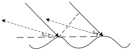
Figure 1.
Bragg scattering mechanism.
According to the Bragg scattering theory, the bistatic sea clutter echo spectrum is primarily made up of two narrow first-order Bragg peaks, as well as the surrounding continuously broadened second-order and higher-order sea clutter. The first-order Bragg peak can be approximately described by two sine signals, while the intensity of second-order and higher-order sea clutter is approximately 10–40 dB lower than that of the first-order Bragg peak [13]. The latter can be simplified with white Gaussian noise.
The theoretical value of the Doppler shift of the bistatic first-order Bragg peak is:
where is the acceleration of gravity, is the radar working wavelength, is incident angle, is scattering angle, and is a bistatic angle.
In practical scenarios, bistatic sea clutter is influenced by various parameters, including ocean current, bistatic angle, and the ionosphere, all of which have a significant impact on the sea clutter spectrum. The current affects the relative speed of the targets on the sea surface. This impact on the sea clutter spectrum can be approximated as a process of spectrum shifting. The ionosphere has non-stationary characteristics, and its influence on electromagnetic waves can be approximated as a modulation effect [14]. As a result, the sea clutter spectrum will be a combination of multiple signal spectra. In addition, the bistatic angle is a variable for each clutter unit, and it affects the formation of first-order sea clutter by causing all sea waves that meet the Bragg resonance condition to undergo Bragg resonance. Then, the corresponding Doppler shift will be superimposed on the sea clutter spectrum, which will inevitably exacerbate spectrum peak splitting and spectrum broadening [15].
Considering the influence of ocean current, the Doppler shift of the bistatic first-order Bragg peak is:
where refers to the radial velocity of the current velocity, which is the velocity component of the current velocity vector on the bisector of the bistatic angle of the scattering point, towards or away from the baseline. Considering that the height of the receiver is usually very low, which is negligible compared with the height of the spaceborne or satellite radiation source. Therefore, the scattering angle is approximated as 0°, and is replaced by “1”.
Considering the combined effects of ionosphere and bistatic angle, the sea clutter spectrum will be the superposition of multiple signal spectra:
where is the sea clutter spectrum, is number of sea clutter, is amplitude of the th clutter, and is frequency deviation.
Figure 2 shows the comparison between the ideal bistatic first-order sea clutter spectrum and the spectrum affected by interference. It can be clearly seen that the sea clutter spectrum has a spectrum shift and a slight spectrum broadening at this time.
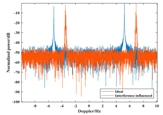
Figure 2.
The comparison between the ideal bistatic first‐order sea clutter spectrum and the spectrum affected by interference.
For the ship target on the sea, its speed is generally slow, and it can be regarded as a uniform motion in a short time. Therefore, the target echo can also be modelled as a sinusoidal signal. If other interference signals are ignored, the received echo is mainly composed of target echo , sea clutter , and Gaussian noise . Therefore, can be expressed as:
2.2. Overview of Compressed Sensing
Compressed sensing was initially proposed by Donoho and Tao [16,17]. The fundamental idea of this theory is: if the signal can be represented sparsely or approximately sparsely in a particular transformation domain, a low-dimensional measurement matrix can be designed to project the signal from the high-dimensional space to the low-dimensional space. A sparse reconstruction algorithm can then be applied to recover the original signal with high probability from a small number of projected values. Compressed sensing can be simply summarized into the following three steps:
Step 1. Signal sparse representation. Signal sparsity or near sparsity is the first prerequisite for compressed sensing. The signal can be sparsely represented in a certain transformation domain. There is a sparse vector and a sparse base matrix , which satisfies . “Sparse” refers to the fact that the number of non-zero elements in vector is far less than the length of the vector.
Step 2. Sensing matrix designing. A measurement matrix is used to measure the signal to obtain the observation set , and is the sensing matrix. The measurement matrix must meet the restricted isometry property (RIP) [18]:
where is the sparsity of signal , is the restricted isometric constant (RIC), and [19].
The RIC is usually difficult to calculate. Baraniuk provides an equivalent condition for the RIP condition, which states that the measurement matrix is not related to the sparse basis matrix [20].
Step 3. Sparse signal reconstruction. The exact or approximate solution of signal can be solved by using the optimization problem in the sense of or norm:
Thus, the reconstructed signal can be obtained:
Apparently, the sparsity of the signal is a prerequisite for compressed sensing. In the case of bistatic radar sea target detection echo, the bistatic first-order strong sea clutter occupies only a small number of frequency units, and its frequency distribution is sparse. This echo model meets the reconstruction requirements of compressed sensing. In order to ensure high reconstruction accuracy, the signal is required to have a high signal-to-noise ratio for sparse signal reconstruction under noise background. The clutter-to-noise ratio of strong sea clutter is typically more than tens of dB, which satisfies the reconstruction requirements. Therefore, the proposed compressed sensing optimization for sea clutter reconstruction in this paper is reasonable.
3. The Proposed Method Description
In this section, we study the bistatic sea clutter suppression method based on compression sensing optimization. Following the fundamental steps of compressed sensing, we introduce three parts: sparse representation of echo, optimal design of sensing matrix, and sea clutter reconstruction suppression.
3.1. Sparse Representation of Signal
Sparse representation of signal is the core of compressed sensing. According to the characteristics of the aforementioned echo model, discrete cosine basis (DCT) is used to sparsely represent the echo. However, the fixed sparse base is not completely suitable for many specific signals, which will lead to poor effect of reconstructed signal. To address this problem, we propose a sparse base optimization algorithm based on transfer learning, which converts fixed sparse base into adaptive sparse base. The objective function of the algorithm is as follows:
where is norm, is the identity matrix, and and are regularization parameters. The first term of the objective function is the loss term of data, the second term is the sparse constraint term, and the third term is the regularization term of transfer learning. We solve the problem (8) through the following two steps:
Step 1. Update sparse representation coefficient : sparse base is fixed and we minimize:
The above optimization problem has the following solution:
where is the soft thresholding operator.
Step 2. Update sparse base : with the sparse representation fixed, we minimize the corresponding sparse base transformation subproblem:
Equation (11) can be expressed in the form of matrix trace:
Because is orthogonal, Equation (11) can be equivalent to:
According to Theorem 4 in [21] and the property of matrix trace , we perform the SVD for to get . Accordingly, we can obtain the unique solution of the above problem:
Then, we can solve the problem by iterating the above update steps alternately. Algorithm 1 shows the description of the sparse base optimization algorithm based on transfer learning.
| Algorithm 1: Sparse Basis Optimization Algorithm Based on Transfer Learning |
| Input: signal , DCT base , Optimized sparse basis matrix , the maximum iterations and regular parameter |
| for k = 1: |
| Calculate sparse representation coefficient by Equation (10); |
| Singular value decomposition of to get |
| Update by Equation (14). |
| end for |
| Output: optimized sparse basis |
3.2. Optimal Design of Sensing Matrix
Designing an effective sensing matrix is a key factor to improve the accuracy of the signal reconstruction in compressed sensing. Recently, various studies have shown that optimizing the sensing matrix by reducing the cross-correlation coefficient between the measurement matrix and the sparse base matrix can significantly improve the quality of signal reconstruction. Therefore, we propose a sensing matrix optimization algorithm based on eigenvalue decomposition and gradient optimization.
In compressed sensing, the observation set , the sensing matrix . The cross-correlation coefficient can be defined as:
where represents after normalization. and represent the column vectors of matrix and , respectively.
Let Gram matrix . The largest off-diagonal element in matrix is the required cross-correlation coefficient. The disadvantage of this definition is that it can only reflect local coherence. Thus, one needs to introduce the global cross-correlation coefficient:
where is the element of Gram matrix .
The definition of the global cross-correlation coefficient is more consistent with RIP criterion. Let the eigenvalue of Gram matrix , according to the trace theory of matrix, . We can reduce the global cross-correlation coefficient by reducing the sum of non-diagonal elements in the Gram matrix:
Because all elements of are 1, problem (17) can be solved by eigenvalue decomposition of the Gram matrix. The optimal solution can be obtained by making the non-zero terms in the eigenvalue , where is the number of rows in the Gram matrix, and is the rank of the Gram matrix. In order to make the signal reconstruction by the above Gram matrix more accurate, the sensing matrix can be further optimized by gradient descent algorithm:
where is the identity matrix, means transposition.
The error is defined as:
After taking the derivative of ε, one obtains . We iteratively update the sensing matrix by setting the step size:
After each iteration, the sensing matrix column is unitized. Algorithm 2 presents a description of the sensing matrix optimization algorithm based on eigenvalue decomposition and gradient descent.
| Algorithm 2: Optimization of Sensing Matrix Based on Eigenvalue Decomposition and Gradient Descent |
| Input: Optimized sparse basis matrix , measurement matrix , identity matrix , step , the maximum iterations and iteration threshold |
| 1. Initial sensing matrix , unitize to get |
| 2. Construction Gram matrix , eigenvalue decomposition of to get |
| 3. Replace all non-zero elements in matrix with to get a matrix |
| 4. Decompose matrix to get |
| 5. Construct a new Gram matrix |
| 6. Obtain initial sensing matrix |
| 7. Iterative optimization of sensing matrix |
| Output: Optimized sensing matrix |
3.3. Sea Clutter Reconstruction Suppression
In this section, the orthogonal matching pursuit algorithm (OMP) is used [22] to reconstruct the bistatic first-order sea clutter, which is then cancelled and suppressed after reconstruction. The flowchart of bistatic sea clutter suppression method based on compressed sensing optimization is shown in Figure 3.
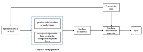
Figure 3.
The flowchart of bistatic sea clutter suppression method based on compressed sensing optimization.
In conjunction with the optimization algorithm presented in the previous two sections, the implementation steps of the sea clutter suppression method based on compression sensing optimization proposed in this paper are as follows:
Step 1. Initialization: the received echo , initial sparse base matrix , measurement matrix , regularization parameter and β;
Step 2. Sparse base optimization: use the sparse base optimization algorithm based on transfer learning to obtain the optimized adaptive sparse base matrix ;
Step 3. Sensing matrix optimization: use the sensing matrix optimization algorithm based on eigenvalue decomposition and gradient descent to obtain the optimized sensing matrix ;
Step 4. Sea clutter reconstruction: Substitute the adaptive sparse base matrix obtained in step 2 and sensing matrix obtained in step 3 into OMP algorithm to reconstruct sea clutter;
Step 5. Cancellation and suppression: cancel the original signal and the reconstructed sea clutter signal to achieve the purpose of sea clutter suppression.
4. Simulation
In this section, we carry out two simulation experiments to verify the effectiveness of the proposed method. In Experiment 1, we investigate the suppression effect of bistatic sea clutter with varying degrees of spectrum peak splitting and broadening at different signal-to-clutter ratios. In Experiment 2, we simulate bistatic sea surface moving target detection and compare the results before and after sea clutter suppression.
4.1. Simulation Experiment 1
Based on the analysis and modeling of signals in Section 2.1, we simulate and construct two sets of mixed echoes consisting of target reflection signals, bistatic sea clutter, and thermal noise. Subsequently, we reconstruct and suppress the sea clutter in the mixed echo. The basic simulation parameters are: radar operating frequency ; Bragg peak frequency ; the target Doppler frequency is ; the target reflection signal and sea clutter signal-to-clutter ratio of two sets of mixed echoes are and , respectively; Meanwhile, the degree of peak splitting and spectral broadening under SCR2 conditions is more severe than that under SCR1 conditions.
Figure 4 shows the comparison of echo power spectra before and after sea clutter suppression using different algorithms under the condition of . The degree of sea clutter spectrum peak splitting and spectrum broadening is relatively slight.
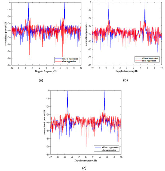
Figure 4.
The comparison of echo power spectra before and after sea clutter suppression using different algorithms under the condition of
: (a) comparison of root method before and after suppression, (b) comparison of SVD method before and after suppression, (c) comparison of the proposed method before and after suppression.
From Figure 4, it is evident that without sea clutter suppression, the bistatic first-order sea clutter is obviously stronger than target reflection signals, and the sea clutter component occupies the main part of the range unit signal. Both the traditional root method and the SVD method have a certain suppression effect on the bistatic first-order sea clutter. Obviously, the power of the first-order sea clutter Bragg peak and the broadened sea clutter near Bragg peak significantly reduced after the cancellation and suppression. Further, Figure 4a–c strongly illustrates that the proposed method has a better suppression effect. Applying this method to suppress sea clutter, the frequency unit where the target signal is located is 2.1 dB higher than the highest value of the other frequency domain units, which makes it easier to extract target information in subsequent processing.
Figure 5 shows the comparison of echo power spectra before and after sea clutter suppression using different algorithms under the condition of . The degree of sea clutter spectrum peak splitting and spectrum broadening is relatively serious.
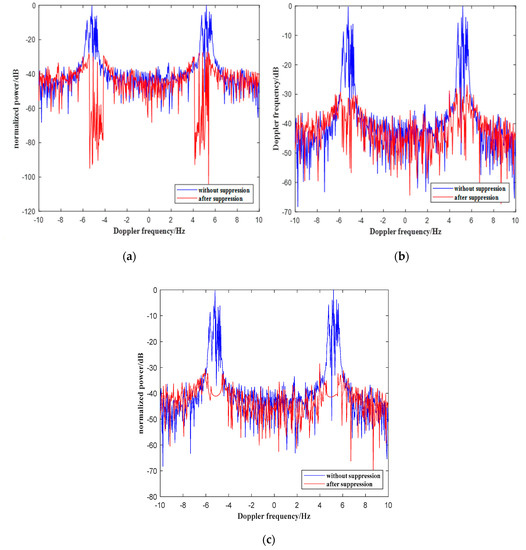
Figure 5.
The comparison of echo power spectra before and after sea clutter suppression using different algorithms under the condition of : (a) comparison of root method before and after suppression, (b) comparison of SVD method before and after suppression, (c) comparison of the proposed method before and after suppression.
Comparing the processing effects of three different algorithms in Figure 5a–c, it can be seen that the root method is basically the same as the SVD method. After the suppression processing by the two traditional methods, the power of the strongest frequency unit in the remaining sea clutter is equivalent to the power of the target reflection signal, but the root method has a large frequency estimation error. By contrast, the proposed method has a significantly better suppression effect because it can accurately reconstruct the broadened first-order sea clutter interference signal. Consequently, the remaining components of sea clutter after reconstruction and cancellation are substantially reduced. Following suppression by this method, the frequency unit where the target reflection signal is located is 4 dB higher than the highest value of the other clutter frequency domain units. Therefore, it is easier to extract target information in subsequent processing.
These three methods essentially reconstruct sea clutter through parameter estimation, and then utilize the reconstructed results to cancel and suppress. Here, we compare the performance of three methods with the sea clutter Bragg peak Doppler frequency estimation error, interference reduction amplitude, and the difference value of power between the target and the maximum clutter as the metrics. Taking as an example, we repeat the experiment 200 times, presenting the mean values of the three metrics in Table 1.

Table 1.
Performance comparison.
Based on Table 1, it is evident that the proposed method can effectively decrease the estimation error in Bragg peak Doppler frequency, while enhancing the performance of interference suppression when compared to the two conventional methods.
4.2. Simulation Experiment 2
In Experiment 2, we simulate the scene of bistatic sea surface target detection, as depicted in Figure 6. In actual sea surface target detection, sea clutter is not only affected by the ionosphere and bistatic angle, but also influenced by ocean currents. The impact of ocean currents on the sea clutter spectrum can be approximated as a process of spectrum shift, resulting in the formation of sea clutter interference in a larger frequency band. The basic simulation parameters are: radar operating frequency ; the distance between the sea surface target and the receiver is ; the target Doppler frequency is . We simulate and generate the bistatic first-order sea clutter broadened by interference, and the signal-to-clutter ratio of target reflection signal and sea clutter is . Figure 7 shows the range Doppler spectrum without sea clutter suppression processing. In order to clearly demonstrate the comparison of results before and after sea clutter suppression, Figure 8 shows the power spectrum at the distance point where the target is located.
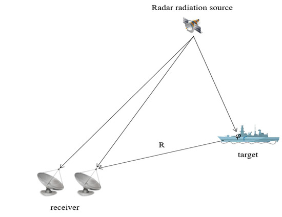
Figure 6.
The diagram of bistatic sea surface target detection.
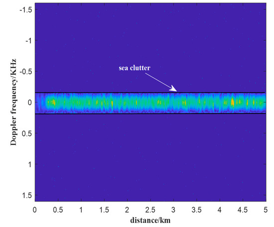
Figure 7.
The range Doppler spectrum without sea clutter suppression processing.
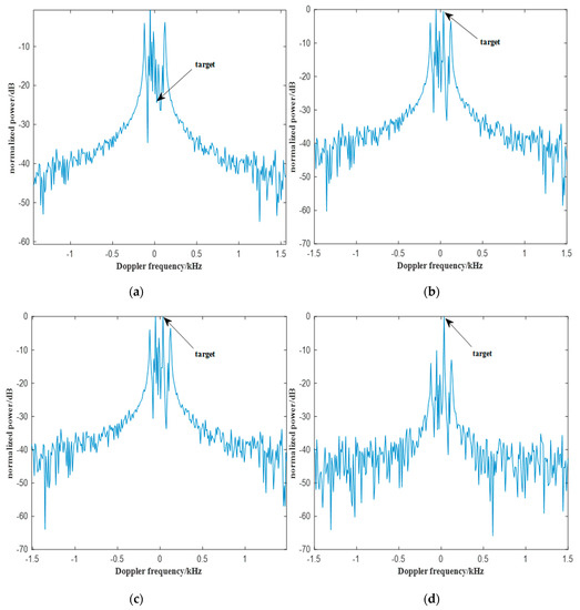
Figure 8.
Comparison of echo power spectra after suppression using different algorithms: (a) without suppression, (b) root method, (c) SVD method, (d) the proposed method.
From Figure 7, it is apparent that there are distinct bands of sea clutter present in the range Doppler spectrum prior to sea clutter suppression. The interference caused by the sea clutter is quite substantial, completely obscuring any target signal within these bands.
Figure 8a shows the results without sea clutter suppression. As can be seen, the target is entirely obscured by the sea clutter, making it challenging to distinguish from the surrounding clutter. Figure 8b–d depicts the results after sea clutter suppression using root method, SVD method, and the proposed method, respectively. In comparison, the method proposed in this paper demonstrates superior suppression performance and more prominent target detection effect.
5. Conclusions
In this paper, we investigate the problem of bistatic sea clutter suppression and propose a new bistatic sea clutter suppression method based on compressed sensing optimization. First, we analyzed and modeled the bistatic radar echo and sea clutter. To address the issue of poor reconstruction signal caused by the fixed sparse basis, we propose a sparse basis optimization algorithm based on transfer learning, which obtains an optimized adaptive sparse basis. Furthermore, we propose a sensing matrix optimization algorithm using eigenvalue decomposition and gradient descent to optimize the sensing matrix. The adaptive sparse basis and the optimized sensing matrix can improve the reconstruction accuracy of sea clutter, and then improve the effect of sea clutter cancellation and suppression. The simulation results demonstrate that the proposed method has a good effect on suppressing bistatic sea clutter. Compared with other radiation sources, spaceborne or satellite radiation sources have unique advantages in the detection of bistatic sea surface target detection and the monitoring of the sea surface, such as wide coverage and work around the clock. In this context, the bistatic sea clutter suppression method proposed in this paper has great practical significance.
Author Contributions
Investigation, J.L.; methodology, J.L.; validation, J.L.; writing—original draft, J.L.; writing—review and editing, Z.P. All authors have read and agreed to the published version of the manuscript.
Funding
This article received no external funding.
Institutional Review Board Statement
Not applicable.
Informed Consent Statement
Not applicable.
Data Availability Statement
Not applicable.
Acknowledgments
Thanks for some guidance and suggestions from Peng.
Conflicts of Interest
The authors declare no conflict of interest.
References
- Rosenberg, L.; Watts, S.; Greco, M.S. Modeling the Statistics of Microwave Radar Sea Clutter. IEEE Aerosp. Electron. Syst. Mag. 2019, 34, 44–75. [Google Scholar] [CrossRef]
- Zhang, X.W.; Yang, D.D.; Guo, J.X.; Zuo, L. Weak Moving Target Detection Based on Short-Time Fourier Transform in Sea Clutter. In Proceedings of the 2019 IEEE 4th International Conference on Signal and Image Processing (ICSIP), Wuxi, China, 19–21 July 2019; pp. 415–419. [Google Scholar] [CrossRef]
- Bi, X.; Guo, S.; Yang, Y.; Shu, Q. Adaptive Target Extraction Method in Sea Clutter Based on Fractional Fourier Filtering. IEEE Trans. Geosci. Remote Sens. 2022, 60, 1–9. [Google Scholar] [CrossRef]
- Duk, V.; Rosenberg, L.; Ng, B.W.H. Target Detection in Sea-Clutter Using Stationary Wavelet Transforms. IEEE Trans. Aerosp. Electron. Syst. 2017, 53, 1136–1146. [Google Scholar] [CrossRef]
- Meiyan, P.A.; Jun, S.U.; Yuhao, Y.A.; Dasheng, L.I.; Sudao, X.I.; Shengli, W.A.; Jianjun, C.H. Improved TQWT for marine moving target detection. J. Syst. Eng. Electron. 2020, 31, 470–481. [Google Scholar] [CrossRef]
- Poon, M.W.Y.; Khan, R.H.; Le-Ngoc, S. A singular value decomposition (SVD) based method for suppressing ocean clutter in high frequency radar. IEEE Trans. Signal Process. 1993, 41, 1421–1425. [Google Scholar] [CrossRef] [PubMed]
- Chen, Z.; He, C.; Zhao, C.; Xie, F. Using SVD-FRFT Filtering to Suppress First-Order Sea Clutter in HFSWR. IEEE Geosci. Remote Sens. Lett. 2017, 14, 1076–1080. [Google Scholar] [CrossRef]
- Anderson, S.J.; Abramovich, Y.I. A unified approach to detection, classification, and correction of ionospheric distortion in HF sky wave radar systems. Radio Sci. 1998, 33, 1055–1067. [Google Scholar] [CrossRef]
- Root, B. HF Radar Ship Detection through Clutter Cancellation. In Proceedings of the 1998 IEEE Radar Conference, RADARCON’98. Challenges in Radar Systems and Solutions (Cat. No.98CH36197), Dallas, TX, USA, 14 May 1998; pp. 281–286. [Google Scholar] [CrossRef]
- Nguyen, S.T.N.; Al-Ashwal, W.A. Sea Clutter Mitigation Using Resonance-Based Signal Decomposition. IEEE Geosci. Remote Sens. Lett. 2015, 12, 2257–2261. [Google Scholar] [CrossRef]
- Farshchian, M. Target Extraction and Imaging of Maritime Targets in the Sea Clutter Spectrum Using Sparse Separation. IEEE Geosci. Remote Sens. Lett. 2017, 14, 232–236. [Google Scholar] [CrossRef]
- Rosenberg, L.; Duk, V.; Ng, B.W.H. Detection in Sea Clutter Using Sparse Signal Separation. IEEE Trans. Aerosp. Electron. Syst. 2020, 56, 4384–4394. [Google Scholar] [CrossRef]
- Chen, S.; Gill, E.W.; Huang, W. A High-Frequency Surface Wave Radar Ionospheric Clutter Model for Mixed-Path Propagation with the Second-Order Sea Scattering. IEEE Trans. Antennas Propag. 2016, 64, 5373–5381. [Google Scholar] [CrossRef]
- Li, Y.J.; Wei, Y.S. Xu, R.Q. Simulation analysis and experimentation study on sea clutter spectrum for high-frequency hybrid sky-surface wave propagation mode. IET Radar Sonar Navig. 2014, 8, 917–930. [Google Scholar] [CrossRef]
- Gill, E.; Huang, W.; Walsh, J. The Effect of the Bistatic Scattering Angle on the High-Frequency Radar Cross Sections of the Ocean Surface. IEEE Geosci. Remote Sens. Lett. 2008, 5, 143–146. [Google Scholar] [CrossRef]
- Donoho, D.L. Compressed sensing. IEEE Trans. Inf. Theory 2006, 52, 1289–1306. [Google Scholar] [CrossRef]
- Candes, E.J.; Romberg, J.; Tao, T. Robust uncertainty principles: Exact signal reconstruction from highly incomplete frequency information. IEEE Trans. Inf. Theory 2006, 52, 489–509. [Google Scholar] [CrossRef]
- Eldar, Y.C.; Mishali, M. Robust Recovery of Signals from a Structured Union of Subspaces. IEEE Trans. Inf. Theory 2009, 55, 5302–5316. [Google Scholar] [CrossRef]
- Davies, M.E.; Gribonval, R. Restricted Isometry Constants Sparse Recovery Can Fail for . IEEE Trans. Inf. Theory 2009, 55, 2203–2214. [Google Scholar] [CrossRef]
- Baraniuk, R.G.; Cevher, V.; Duarte, M.F.; Hegde, C. Model-Based Compressive Sensing. IEEE Trans. Inf. Theory 2010, 56, 1982–2001. [Google Scholar] [CrossRef]
- Zou, H.; Hastie, T.; Tibshirani, R. Sparse Principal Component Analysis. J. Comput. Graph. Stat. 2006, 15, 265–286. [Google Scholar] [CrossRef]
- Tropp, J.A. Greed is good: Algorithmic results for sparse approximation. IEEE Trans. Inf. Theory 2004, 50, 2231–2242. [Google Scholar] [CrossRef]


Disclaimer/Publisher’s Note: The statements, opinions and data contained in all publications are solely those of the individual author(s) and contributor(s) and not of MDPI and/or the editor(s). MDPI and/or the editor(s) disclaim responsibility for any injury to people or property resulting from any ideas, methods, instructions or products referred to in the content. |
© 2023 by the authors. Licensee MDPI, Basel, Switzerland. This article is an open access article distributed under the terms and conditions of the Creative Commons Attribution (CC BY) license (https://creativecommons.org/licenses/by/4.0/).