A Comprehensive Study of Machine Learning Application to Transmission Quality Assessment in Optical Networks

Abstract

This paper examines applying machine learning to the assessment of the quality of the transmission in optical networks. The motivation for research into this problem derives from the fact that the accurate assessment of transmission quality is key to an effective management of an optical network by a network operator. In order to facilitate a potential implementation of the proposed solution by a network operator, the training data for the machine learning algorithms are directly extracted from an operating network via a control plane. Particularly, this work focuses on the application of single class and binary classification machine learning algorithms to optical network transmission quality assessment. The results obtained show that the best performance can be achieved using gradient boosting and random forest algorithms.

1. Introduction

Over the last decades, the demand for traffic and bandwidth in optical backbone networks has constantly increased. Therefore, there is a need for efficient use of available network resources. Apart from introducing new technological solutions enabling higher transmission rates, a network operator needs to frequently reconfigure and reoptimize the network in order to minimize capital expenditure (Capex) and operational expenditure (Opex) [1,2,3,4,5]. Efficient use of available resources is of particular importance for dense wavelength division multiplexed (DWDM) networks [6]. With their high bandwidth and low cost, DWDM optical networks form the platform for implementing core physical infrastructure by all major operators worldwide. They are currently penetrating important new telecoms markets, such as the the data market and the access segment. Consequently, DWDM network management is one of the main problems faced by optical network operators whereby an accurate assessment of transmission quality is a necessary prerequisite to any realistic network reconfiguration plan. In this paper, we have therefore focused on the problem of quality assessment in a DWDM network and propose a solution, which can be relatively easily implemented by a network operator. This solution involves applying machine learning algorithms to a database that contains relevant information about the network traffic and can be conveniently extracted from the DWDM system via the control plane.

More specifically, this paper applies machine learning (ML) algorithms to a database that has been taken directly by the control plane from a next-generation optical network from a large telecom network operator within the software-defined network (SDN) paradigm. ML techniques may prove helpful in improving the management of resources within a modern optical network mainly because of their ever increasing complexity of infrastructure. An intelligent selection of the parameter values may improve the overall network performance.

The use of data directly from an operational optical network, collected through a control plane and as input to ML algorithms is, not straightforward due to the large data size and class imbalance. This class imbalance arises because practically all links are working in an operational optical network, and nobody attempts to set up or especially keep allocated a link that, for instance, has the bit error rate too high. Even though there is some knowledge regarding nonworking links within a corporation, it is usually very scarce and poorly documented. Furthermore, experiments on synthetic data may lead to overoptimistic predictive performance estimates as well as a failure to identify important obstacles. Therefore, we propose a specially tailored approach using ML algorithms to solve this problem and compare binary classification algorithms combined with different class imbalance compensation techniques with single-class classification algorithms. In our solution, all attributes are divided into subsets, and ML algorithms are compared for each subset of parameters. As the measure of performance of selected machine learning algorithms, receiver operating characteristics (ROC) and precision-recall curves were selected. When compared with [7,8], this study presents a comprehensive approach to investigate the prediction quality of machine learning algorithms applied to optical network design. We used an extended set of classification algorithms and a combined dataset originating from two networks. We systematically investigated the predictive utility of multiple attribute subsets, differing in the scope of physical properties of network paths, and performed hyperparameter tuning to ensure that each algorithm reveals its full predictive power potential.

The paper is organized as follows. Section 2 provides a review of the literature and papers in this scientific field. Section 3 presents the data collection methodology, while Section 4 describes the figures of merit of machine learning algorithms. The results and discussion of the optical network simulations are presented in Section 5. The final summary is provided in Section 6.

2. Related Work

SDN and knowledge-based networking (KDN) paradigms are instrumental in implementing frequent network reconfiguration and reoptimization within a DWDM network [9,10]. Central to SDN and KDN is an accurate estimation of transmission quality [11,12]. Therefore, a number of ML-based models have been proposed that synthetically create the database and apply ML to such data [13,14]. However, modeling methods used to create synthetic databases often place too high computational requirements for real-time prediction, making them unscalable to large networks. Moreover, these models rely on a number of parameters that may not be available to a network operator. In [15,16], the authors claim that ML technology will become an important means to providing indispensable technical support to further increase communication capacity and improve future communication stability by effectively identifying physical impairments in the network [17]. In the new generation passive optical networks (PONs) [18], ML-based algorithms have also been successfully applied, particularly to the load-balancing problem [19].

Here, we follow an alternative approach to the application of ML to the automatic reconfiguration of an optical network that relies only on the data that are available to a network operator via the control plane. Such an approach is distinct from the one followed in [10,13]. Similar lightpath QoT estimation problems were also addressed in [20,21], whereby the solution presented there mainly focused on an application of the SVM classifier; meanwhile, in [22], the authors used the random forest algorithm. A similar approach was also used in [23]. In all these cases, the system was trained and tested on artificial data, which differs qualitatively from the approach taken in this paper. As already mentioned here, we rely only on the data that are available to a network operator via the control plane. The resulting training dataset is intrinsically imbalanced and, as already mentioned, potentially small, thus making the adoption of ML methods that are specially tailored for handling imbalanced datasets necessary.

In [24], the author compared different means to dealing with class imbalance, including data resampling and one-class classification. It was concluded that binary classification with imbalance compensation is superior to single-class classification. A similar problem to the one presented here was discussed in [25]. The results presented in this work suggest that binary classification may be more effective than single-class classification for data with complex multimodal distributions. In contrast, Lee and Cho used single-class classification for unbalanced data and showed that it could outperform binary classification if the unbalanced factor is high [26]. Their work inspired further research into the utility of binary and one-class algorithms for optical network path classification, such as in [7,8]. The results suggested that the one-class approach can be a viable alternative to standard binary classification in this application domain. However, binary classification with class imbalance compensated by class weights still works reasonably well, and the more refined SMOTE [27] and ROSE [28] techniques do not lead to improved predictive performance. This work, therefore, revisits the binary classification approach using class weights for imbalance compensation. We extensively and systematically explore the potential of improving the prediction quality by evaluating the utility of different attribute subsets corresponding to different physical network path properties, using a broader scope of classification algorithms, and tuning their hype-parameters.

The literature are includes interesting attempts use artificial neural networks (ANNs), where the inputs are channel loadings and launch power settings [29] or source-destination nodes, link occupation, modulation format, path length, and data rate [30]. This work, however, focuses primarily on standard ML algorithms, known to be well suited for tabular data and capable of creating useful models even from small and imbalanced datasets. With that being said, the multilayer perceptron, as the standard general-purpose neural network architecture, is included in the experiments as well.

3. Problem Formulation

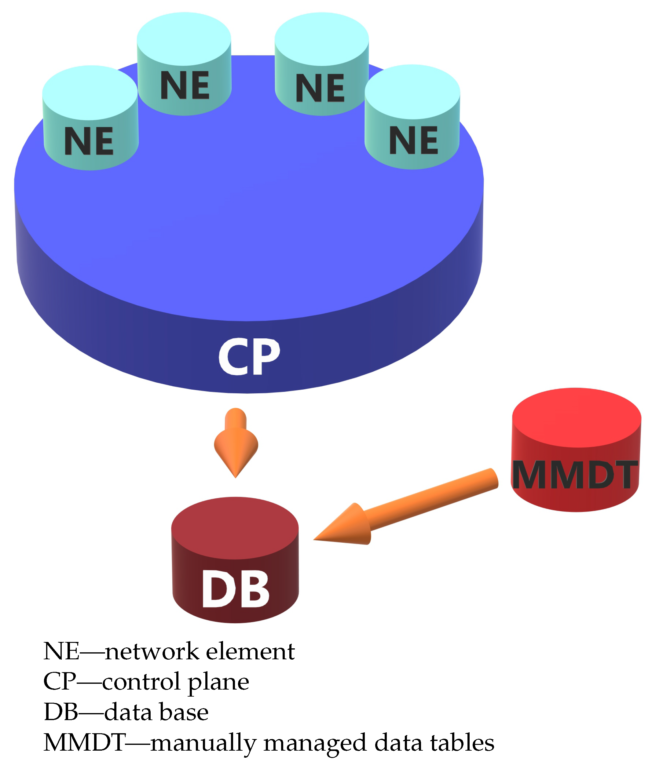
This work approaches transmission quality assessment as a binary classification task in which a network path is to be classified as “good” (successfully deployed, i.e., meeting transmission quality requirements or “bad” (not successfully deployed, i.e., not meeting transmission quality requirements). This makes it possible to apply machine learning algorithms to create models providing class or class probability predictions based on available path attributes.

It is a well-established fact in the area of machine learning that a suitable selection of attributes may significantly improve the accuracy of predictions. In this contribution, therefore, the problem of attribute selection for machine learning algorithms used in models predicting the quality of transmission in optical point-to-point connections of a DWDM network is studied. Two approaches can potentially be considered when selecting attributes. One of them is quantitative in nature and is based on the classical approach used in machine learning that finds the attributes that are best correlated with the prediction results. The other is rather qualitative and aims to exploit the well-established optical transmission theory in optical networks. It has been observed that the presence of physical phenomena such as fiber attenuation, optical signal attenuation in a DWDM node, polarization-dependent loss, EDFA amplifier noise, chromatic dispersion, polarization dispersion, and nonlinear phenomena, including especially four-wave mixing, is related to the quality of transmission in the optical links of a point-to-point DWDM network. One would therefore expect that there exists a mapping that relates the parameters that characterize these physical phenomena and the quality of transmission in point-to-point DWDM network optical links. Considering such parameters as fiber attenuation, optical signal attenuation in a DWDM node, polarization-dependent loss, EDFA amplifier noise figure, chromatic dispersion, and polarization dispersion, the parameters characterizing nonlinear phenomena present in optical fibers (e.g., the nonlinear fiber coefficient present in the nonlinear Schrodinger equation) should therefore be instrumental in evaluating the quality of transmission in point-to-point DWDM network optical links. However, these parameters are not readily available to a DWDM network operator via the control plane. Further, in general, it is not a trivial matter to accurately extract the values of such a set of parameters from an operating DWDM network primarily because it would require a major effort and prompt a significant increase in operational expenditure (Opex), which would be extremely difficult to justify at a DWDM network operator management board level. Other methods, therefore, need to be considered. An approach that seems pragmatic and hence is investigated here consists in first collecting a set of parameters characterizing a DWDM network, which are readily available via the DWDM network control plane and thus can be used to automatically create a database that characterizes the considered DWDM network.

In this study, the data were directly collected from the network monitoring system of the real optical network of a large telecom operator. It was assumed that the optical channels (lightpaths) operate in C-band. The network is located in Poland, with nodes corresponding to network elements located in the main cities of the country. The network is extensive, with an area of approximately 1000 km in diameter. The longest distance between the two most distant nodes is 120 km, and the average distance between them is 60 km.

3.1. Data

The considered optical network uses both coherent and noncoherent transponders. The coherent transponders belong to Ciena’s 6500 family. The transponder transmission rates are 100 Gbit/s, 200 Gbit/s, and 400 Gbit/s. The modulation formats include Quadrature Phase Shift Keying (QPSK) and Quadrature Amplitude Modulation (QAM): 16 QAM, 32 QAM and 64 QAM. The noncoherent transponders belong to Nokia’s 1626 family and have bit rates of 2.5 Gbit/s and 10 Gbit/s.

A schematic of the data preparation process is shown in Figure 1. Figure 2 and in detail, in Figure 3 are provided to facilitate the understanding of the attributes used, i.e.,: hop, hop length, path, and transponder. The dataset contains 1070 optical channels (paths), for which 18 were unsuccessful paths (“bad”), and (1052) were successfully deployed (“good”).

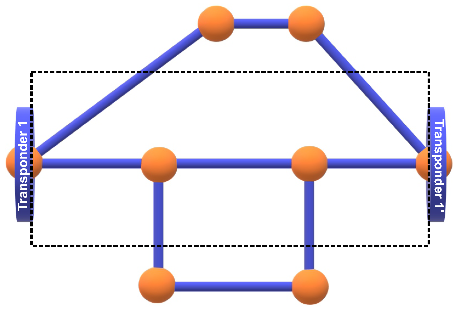
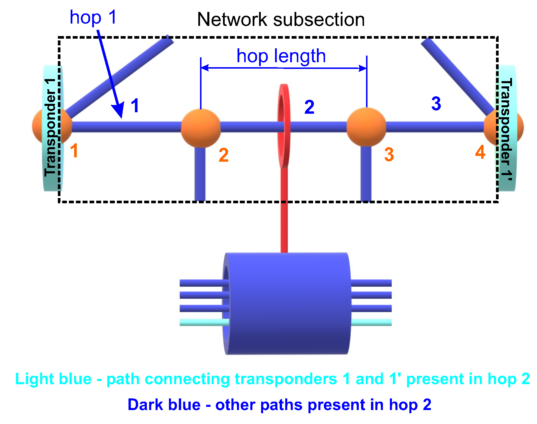
3.1.1. Path Description

Optical channels (lightpaths) have been described by attributes. The hop_lengths attribute gives the length of each hop that forms an optical channel from its origin transponder to the end. This is an important property because the signal-to-noise ratio depends on the length of the fiber that connects the two transponders. There are usually more active and commercial wavelengths in each such edge (hop). This is because these wavelengths are used by paths other than the ones occupied by the path under consideration. All these optical channels in an edge (hop) interact with each other through so-called nonlinear phenomena, such as four-wavelength mixing, which affects the quality of transmission.

With this in mind, the num_of_paths_in_hops attribute was considered, which gives the number of neighboring wavelengths (optical channels) of the network in a given edge. The attribute hop_losses denotes the attenuation and, therefore, the optical losses in the considered edge. Again, hop losses affect the signal-to-noise ratio. Hence, the corresponding property is included. Another property, number_of_hops, denotes how many edges occur in a given optical channel from the origin transponder to the destination transponder. The number of hops affects the signal-to-noise ratio due to the optical regeneration taking place at the network node.

The last two properties are closely related to the specific type of transponder used. The transponder_modulation property stores information about the modulation format of the transponder, e.g., 64QAM or QPSK. Since the modulation format is closely related to the sensitivity of the receiver, this property is, therefore, very important. On the other hand, the property transponder_bitrate is quite self-explanatory and provides the bit rate of a given transponder. The bit rate of the transponder also affects the sensitivity of the receiver and is therefore also included.

3.1.2. Vector Representation

Path descriptions were transformed to a vector representation using an aggregation-based technique. Each of the available edge properties can be aggregated by calculating the following functions over all edges in the path:

• sum (*edge property name*.sum);
• mean (*edge property name*.avg);
• median (*edge property name*.med);
• standard dev. (*edge property name*.std);
• minimum (*edge property name*.min);
• maximum (*edge property name*.max);
• first quartile (*edge property name*.q1);
• third quartile (*edge property name*.q3);
• linear correlation with the edge’s ordinal number in the path:
  (*edge property name*.cor).

This gives 27 attributes in addition to the 3 path attributes unrelated to individual edges.

3.1.3. Attribute Subsets

The available attributes as listed in the preceding subsection are divided into three groups shown in

Table 1. Available attributes divided into three groups.

Group Name	Attributes
G1 (path-related)	number_of_hops
G2 (hop-related)	hop_length
	hop_losses
	number_of paths_in_hops
G3 (trans-related)	transponder_bitrate
	transponder_modulation

. Based on the groups shown in Table 1, the attribute subsets presented in

Table 2. Attribute subsets.

Groups Combination	Attribute Subsets
G1	S1
G2	S2
G3	S3
G1 + G2	S4
G1 + G3	S5
G2 + G3	S6
G1 + G2 + G3	S7

were derived and used in simulations.

4. Machine Learning Algorithms

The objective of this work is to investigate the predictive performance of classification models for optical path quality assessment using different sets of attributes describing their properties. Since algorithm properties such as model representations and generalization mechanisms may have substantial impact on their capability of effectively utilizing different sets of attributes, this study uses several different algorithms. This is a relatively diverse and quite broad selection of the most popular classification algorithms, both in research and applications. They are capable of providing the best possible level of prediction quality for tabular data. The algorithms are briefly characterized in the corresponding subsections below. These descriptions highlight their most important properties that make them interesting and useful, justifying their selection for this study. The final subsection presents the applied model evaluation methods.

4.1. Logistic Regression

The logistic regression algorithm uses a generalized linear model representation with a logit link function. Model parameters are fitted by minimizing the logarithmic loss on the training set [31]. The resulting model provides class probability predictions which are well calibrated. The algorithm is relatively resistant to overfitting unless used for high-dimensional data. In the latter case, regularization can be applied to further reduce the risk of overfitting. The internally used solver for logarithmic loss minimization and the type and strength of regularization are controlled by adjustable hyperparameters. Comparing logistic regression, as a relatively simple algorithm with a limited-capacity model space, to more refined classification algorithms makes it possible to verify whether their added complexity pays off in the optical channel application domain.

4.2. Support Vector Machines

Support Vector Machines (SVM) use a linear decision boundary for separating classes but can also fit to linearly inseparable data via separation constraint relaxation (“soft-margin”) and by using kernel functions for implicit input transformation [32,33,34]. The algorithm solves a quadratic programming problem with the objective of classification margin maximization and with constraints controlling the fit to the data. This makes it resistant to overfitting even for small and multidimensional datasets, which is an important advantage in our application domain. Important adjustable hyperparameters include the cost of constraint violation as well as the type and parameters of the kernel function.

Model predictions are obtained based on the decision function proportional to the signed distance of the classified instance to the decision boundary. An optional logistic output transformation known as Platt’s scaling, with parameters adjusted for maximum likelihood, makes it possible to obtain class probability predictions [35].

4.3. Random Forest

The random forest algorithm creates a model ensemble consisting of multiple decision trees, grown based on multiple bootstrap samples from the training data [36]. To make trees in the ensemble more diverse, which is essential for ensemble modeling, split selection is randomized by random attribute sampling at each node. Trees are grown to a maximum or near-maximum depth and remain unpruned, which makes them even more likely to differ. With dozens or hundreds of diversified trees, random forests are usually highly accurate and resistant to overfitting. The algorithm’s sensitivity to hyperparameter settings is limited, making it easy to use, and sometimes tuning the number of trees and the number of attributes randomly drawn for split selection at each node offers some improvement.

Predicted classes are determined by the unweighted voting of class labels predicted by particular trees. Predicted class probabilities can be obtained based on vote distribution. An additional useful capability of the algorithm is providing variable importance values, i.e., measuring the predictive utility of available attributes. The most useful type of variable importance is the mean decrease of accuracy resulting from a random permutation of attribute values, estimated using out-of-bag training instances [37].

4.4. Gradient Boosting

Boosting is another approach to ensemble modeling in which models are created sequentially, with each subsequent model supposed to best contribute to the combined predictive power of the ensemble by compensating for the imperfections of the previously created ones [38,39]. Gradient boosting uses regression trees as ensemble components, grown so as to optimize an ensemble quality function composed of a loss term, which measures the level of fit to the training data, and a regularization term, which penalizes model complexity [40].

Gradient boosting with logarithmic loss and a logit link function is applicable to binary classification. The resulting models usually provide a very high level of prediction quality, on par with or better than that obtained by random forest models. The algorithm is however more prone to overfitting which may occur if too many trees are grown, so setting or tuning the ensemble size requires some care.

4.5. k-Nearest Neighbors

The k-nearest neighbors or k-NN algorithm belongs to the family of memory-based learning algorithms which essentially store the original labeled training data as their only model representation to be used at the prediction phase. In the case of k-NN classification, the true class labels of k training instances closest to the instance for which the prediction is being made are used to determine the predicted class label by voting and are possibly weighted [41]. The algorithm can be used with arbitrary distance measures, with the Euclidean distance being the most popular choice, unless some properties of the application domain knowledge suggest another more appropriate metric. Vote weights, if used, are typically inversely proportional to the distance between the neighbor and the instance for which the prediction is being made. Vote distribution can be also used to obtain class probability predictions.

With a distance measure well suited to the domain and appropriately selected k to control the risk of overfitting, the resulting predictions may be competitive to those of other more refined algorithms. The computational expense of nearest neighbor search is mitigated by using tree structures for fast indexing.

4.6. Multilayer Perceptron

The multilayer perceptron or MLP algorithm is the most widely used general purpose neural network architecture, in which a classification or regression model is represented by a set of neuron-like processing units organized into layers with feed-forward weighted connections [42]. Using nonlinear activation functions in one or more layers, such models can overcome the limitations of linear or logistic regression. The logistic of hyperbolic tangent functions are standard activation function choices, but recently the ReLU (rectified linear unit) function has become more popular, as it makes it possible to avoid the vanishing gradient problem in networks with more layers [43].

When applied to classification, the multilayer perceptron algorithm can be trained to minimize the logarithmic loss. While slower and more sensitive to parameter setup than logistic regression, it can represent more complex relationships between input attributes and class probabilities.

4.7. Model Evaluation

The $n\times k$-fold cross-validation procedure was used to evaluate models. It effectively uses all available data for both model creation and model evaluation by randomly dividing into k equal-sized subsets. Each of these serves as a test set to evaluate the model created at the union of the other subsets. This results in low evaluation bias and variance. For even further variance reduction, this process is repeated n times. The true class labels and predictions for all $n\times k$ iterations are then combined to calculate prediction quality measures. Due to significant class imbalance, a random subdivision into k subsets by stratified sampling was performed. Roughly the same number of minority class instances in each subset was retained. We used $k=5$ and $n=50$. While the latter may appear untypically large, it is both computationally affordable and desirable when working with small data for the maximum reliability of model evaluation.

Since misclassification error or classification accuracy are not useful for data with imbalanced classes and since all algorithms used for the experimental study can deliver class probability predictions besides class label predictions, predictive performance was measured using precision-recall (PR) and receiver operating characteristic (ROC) curves. They visualize all possible model operating points, obtained by comparing class probability predictions against the whole range of possible threshold values. In the case of precision-recall curves, these points correspond to different tradeoffs between the precision (the share of positive class predictions that are correct) and the recall (the share of positive instances which are correctly predicted as positive). In the case of ROC curves, they correspond to different tradeoffs between the true-positive rate (the same as the recall) and the false-positive rate (the share of negative instances incorrectly predicted to be positive). The “bad” class was considered positive, and “good” class was considered negative for this evaluation. The corresponding areas under the curve (PR AUC, ROC AUC) served as the overall aggregated measures of predictive performance over all possible cutoff thresholds.

These two measures may favor different models. PR curves are much more sensitive to false positives under class imbalance, and to maximize PR AUC, which is the average precision over the whole range of recall values, a model has to prevent a substantial share of its “bad” class predictions from being incorrect, even if it also prevents it from correctly detecting some of truly “bad” paths. To maximize ROC AUC, on the other hand, it is sufficient to avoid making incorrect “bad” class predictions for a substantial share of paths that are actually “good”, which makes it possible to focus on detecting as many “bad” paths as possible. The preference for one or the other may depend on the particular application scenario and the corresponding business costs of incorrect predictions. We therefore present both these evaluations, and separately optimize hyperparameters with respect to PR AUC and ROC AUC.

5. Results

The following algorithm implementations were used in the experimental studies that were carried out [44]. For each proposed algorithm, the hyperparameters have been tuned, which are also described in the

Table 3. Hyperparameters tuned for particular algorithms.

Algorithm	Hyperparameter	Values	Default
LR	class_weigth	‘balanced’	None
	solver	‘lbfgs’, ‘liblinear’	‘lbfgs’
	penalty	‘l1’, ‘l2’, ‘elasticnet’	‘l2’
	c	100, 10, 1.0, 0.1, 0.01	1
SVC	class_weigth	None, ‘balanced’	None
	c	0.1, 1, 10, 100	1
	gamma	`scale’, ‘auto’	`scale’
	kernel	‘linear’, ‘rbf’	‘rbf’
RFC	class_weight	None, ‘balanced’	None
	n_estimators	25, 100, 250, 500	100
	min_samples_split	3, 7, 10, 13	2
	max_depth	None, 2, 3, 5	None
GBC	n_estimators	25, 100, 250, 500	100
	min_samples_split	3, 7, 10, 13	2
	max_depth	1, 2, 3, 5	3
KNC	n_neighbors	2, 3, 5, 10, 15	5
	leaf_size	20, 25, 30, 35	30
	p	1, 2	2
MCPL	hidden_layer_sizes	(100), (50), (50,50)	(100)
	activation	‘tanh’, ‘relu’	‘relu’
	solver	‘sgd’, ‘adam’	‘adam’
	alpha	0.0001, 0.05	0.0001
	learning_rate	‘constant’, ‘adaptive’	‘constant’

.

• LR: LogisticRegression:
  • class_weight—weights for handling class imbalance;
  • solver—the algorithm to use in the optimization problem;
  • penalty—regularization type;
  • c—the inverse of regularization strength.
• SVC: SupportVectorClassifier:
  • class_weight—weights for handling class imbalance;
  • c—the cost of constraint violation;
  • gamma—the kernel parameter;
  • kernel—the kernel type to be used in the algorithm.
• RFC: RandomForestClassifier:
  • class_weight—weights for handling class imbalance;
  • n_estimators—the number of trees in the forest;
  • min_samples_split—the number of samples required to split a node;
  • max_depth—the maximum tree depth.
• GBC: GradientBoostingClassifier:
  • n_estimators—the number of trees (boosting iterations);
  • min_samples_split—the number of samples required to split a node;
  • max_depth—the maximum tree depth.
• KNC: KNeighborsClassifier:
  • n_neighbors—the number of neighbors considered when making prediction;
  • leaf_size—the size of the leaf in the neighor search tree;
  • p—the power parameter for the Minkowski metric.
• MLPC: MLPClassifier:
  • hidden_layer_sizes—the number and shapes of hidden layers;
  • activation—the activation function of neurons;
  • solver—the optimization algorithm;
  • alpha—the regularization parameter;
  • learning_rate—the learning step size.

Each algorithm was applied to each attribute subset presented in Section 3.1, with independent hyperparameter tuning in each case. Table 3 presents the most important hyperparameters of particular algorithms that were tuned, along with the range of values considered for tuning and default settings.

Table 4. The best hyperparameter settings for particular algorithms and attribute subsets identified by tuning.

Model	Subset	Best PR Parameters	Best ROC Parameters
LR	$S1$	C = 0.1, class_weight = ‘balanced’, penalty = ‘l1’, solver = ‘liblinear’	C = 100, class_weight = ‘balanced’
	$S2$	C = 0.01, class_weight = ‘balanced’	C = 0.01, class_weight = ‘balanced’, penalty = ‘l1’, solver = ‘liblinear’
	$S3$	C = 0.01, class_weight = ‘balanced’, penalty = ‘l1’, solver = ‘liblinear’	C = 0.01, class_weight = ‘balanced’, penalty = ‘l1’, solver = ‘liblinear’
	$S4$	C = 0.01, class_weight = ‘balanced’	C = 0.01, class_weight = ‘balanced’, penalty = ‘l1’, solver = ‘liblinear’
	$S5$	C = 10, class_weight = ‘balanced’	C = 0.01, class_weight = ‘balanced’
	$S6$	class_weight = ‘balanced’, solver = ‘liblinear’	C = 0.01, class_weight = ‘balanced’, solver = ‘liblinear’
	$S7$	class_weight = ‘balanced’, solver = ‘liblinear’	C = 0.01, class_weight = ‘balanced’, solver = ‘liblinear’
SVC	$S1$	C = 0.1, gamma = ‘auto’	C = 0.1, class_weight = ‘balanced’, kernel = ‘linear’
	$S2$	C = 100	C = 0.1, class_weight = ‘balanced’, gamma = ‘auto’
	$S3$	C = 100, kernel = ‘linear’	C = 0.1, class_weight = ‘balanced’, kernel = ‘linear’
	$S4$	C = 100	C = 0.1, class_weight = ‘balanced’
	$S5$	C = 1, class_weight = ‘balanced’, gamma = ‘auto’	C = 1, class_weight = ‘balanced’, gamma = ‘auto’
	$S6$	C = 0.1, gamma = ‘auto’, kernel = ‘linear’	C = 0.1, class_weight = ‘balanced’
	$S7$	C = 0.1, kernel = ‘linear’	C = 0.1, class_weight = ‘balanced’, gamma = ‘auto’
RFC	$S1$	class_weight = ‘balanced’, max_depth = 2, min_samples_split = 10, n_estimators = 25	max_depth = 2, min_samples_split = 3, n_estimators = 500
	$S2$	min_samples_split = 13	min_samples_split = 7, n_estimators = 500
	$S3$	class_weight = ‘balanced’, min_samples_split = 10	class_weight = ‘balanced’, max_depth = 2, min_samples_split = 10, n_estimators = 500
	$S4$	min_samples_split = 13, n_estimators = 250	max_depth = 5, min_samples_split = 3, n_estimators = 250
	$S5$	max_depth = 3, min_samples_split = 10, n_estimators = 250	max_depth = 5, min_samples_split = 10
	$S6$	min_samples_split = 13, n_estimators = 250	max_depth = 5, min_samples_split = 13, n_estimators = 500
	$S7$	min_samples_split = 13, n_estimators = 500	max_depth = 5, min_samples_split = 3, n_estimators = 500
GBC	$S1$	max_depth = 5, min_samples_split = 12	max_depth = 2, min_samples_split = 12, n_estimators = 25
	$S2$	min_samples_split = 12	min_samples_split = 3, n_estimators = 500
	$S3$	max_depth = 2, min_samples_split = 3, n_estimators = 25	max_depth = 2, min_samples_split = 3, n_estimators = 25
	$S4$	min_samples_split = 8	max_depth = 5, min_samples_split = 3
	$S5$	max_depth = 2, min_samples_split = 12	max_depth = 5, min_samples_split = 8
	$S6$	max_depth = 2, min_samples_split = 12	max_depth = 2, min_samples_split = 3
	$S7$	max_depth = 2, min_samples_split = 12, n_estimators = 250	min_samples_split = 8
KNC	$S1$	leaf_size = 25, n_neighbors = 15	n_neighbors = 15
	$S2$	n_neighbors = 2	leaf_size = 35, n_neighbors = 15, p = 1
	$S3$	n_neighbors = 2, p = 1	leaf_size = 20, n_neighbors = 10, p = 1
	$S4$	leaf_size = 20, n_neighbors = 3	leaf_size = 20, n_neighbors = 15, p = 1
	$S5$	p = 1	n_neighbors = 15, p = 1
	$S6$	n_neighbors = 2	leaf_size = 25, n_neighbors = 15, p = 1
	$S7$	leaf_size = 35, n_neighbors = 2	leaf_size = 20, n_neighbors = 15, p = 1
MLPC	$S1$	solver = ‘sgd’	activation = ‘tanh’, solver = ‘sgd’
	$S2$	activation = ‘tanh’, alpha = 0.05, hidden_layer_sizes = (50), learning_rate = ‘adaptive’	activation = ‘tanh’, learning_rate = ‘adaptive’
	$S3$	activation = ‘tanh’, hidden_layer_sizes = (50,)	activation = ‘tanh’
	$S4$	activation = ‘tanh’, hidden_layer_sizes = (50,50)	activation = ‘tanh’, learning_rate = ‘adaptive’
	$S5$	hidden_layer_sizes = (50,50)	activation = ‘tanh’, hidden_layer_sizes = (50,50)
	$S6$	activation = ‘tanh’	activation = ‘tanh’, hidden_layer_sizes = (50),
			learning_rate = ‘adaptive’
	$S7$	activation = ‘tanh’, alpha = 0.05	activation = ‘tanh’, alpha = 0.05, solver = ‘sgd’

shows the best settings obtained by hyperparameter tuning. Only nondefault values are included. It can be seen that for each algorithm, the best settings usually differ, sometimes substantially, depending on the attribute subset and performance measure used. Despite imbalanced classes, the balanced setting of the class_weights parameter, which is available for most of the algorithms, does not always appear to help. For the multilayer perceptron, a single hidden layer is usually sufficient.

The obtained PR and ROC curves are presented in Figure 4 and Figure 5: each plot corresponds to a single algorithm and presents the curves for different attribute subsets. The values of the corresponding areas under these curves, summarizing the overall predictive performance, are presented in

Table 5. PR AUC values for particular algorithms and attribute subsets.

Model	S1	S2	S3	S4	S5	S6	S7
LR	0.094	0.096	0.189	0.096	0.101	0.167	0.167
SVC	0.148	0.131	0.253	0.128	0.177	0.167	0.162
RFC	0.116	0.385	0.363	0.383	0.238	0.461	0.457
GBC	0.09	0.389	0.356	0.392	0.196	0.448	0.45
KNC	0.144	0.197	0.387	0.202	0.217	0.24	0.22
MLPC	0.117	0.083	0.189	0.101	0.178	0.175	0.175

and

Table 6. ROC AUC values for particular algorithms and attribute subsets.

Model	S1	S2	S3	S4	S5	S6	S7
LR	0.818	0.799	0.687	0.797	0.896	0.898	0.898
SVC	0.816	0.799	0.561	0.795	0.899	0.87	0.872
RFC	0.818	0.856	0.718	0.854	0.897	0.915	0.917
GBC	0.806	0.833	0.72	0.836	0.896	0.891	0.894
KNC	0.683	0.739	0.625	0.737	0.789	0.79	0.797
MLPC	0.816	0.797	0.677	0.789	0.897	0.888	0.885

. For easier comparison, the latter are also visualized by barplots in Figure 6 and Figure 7.

Several conclusions can be drawn from the results obtained:

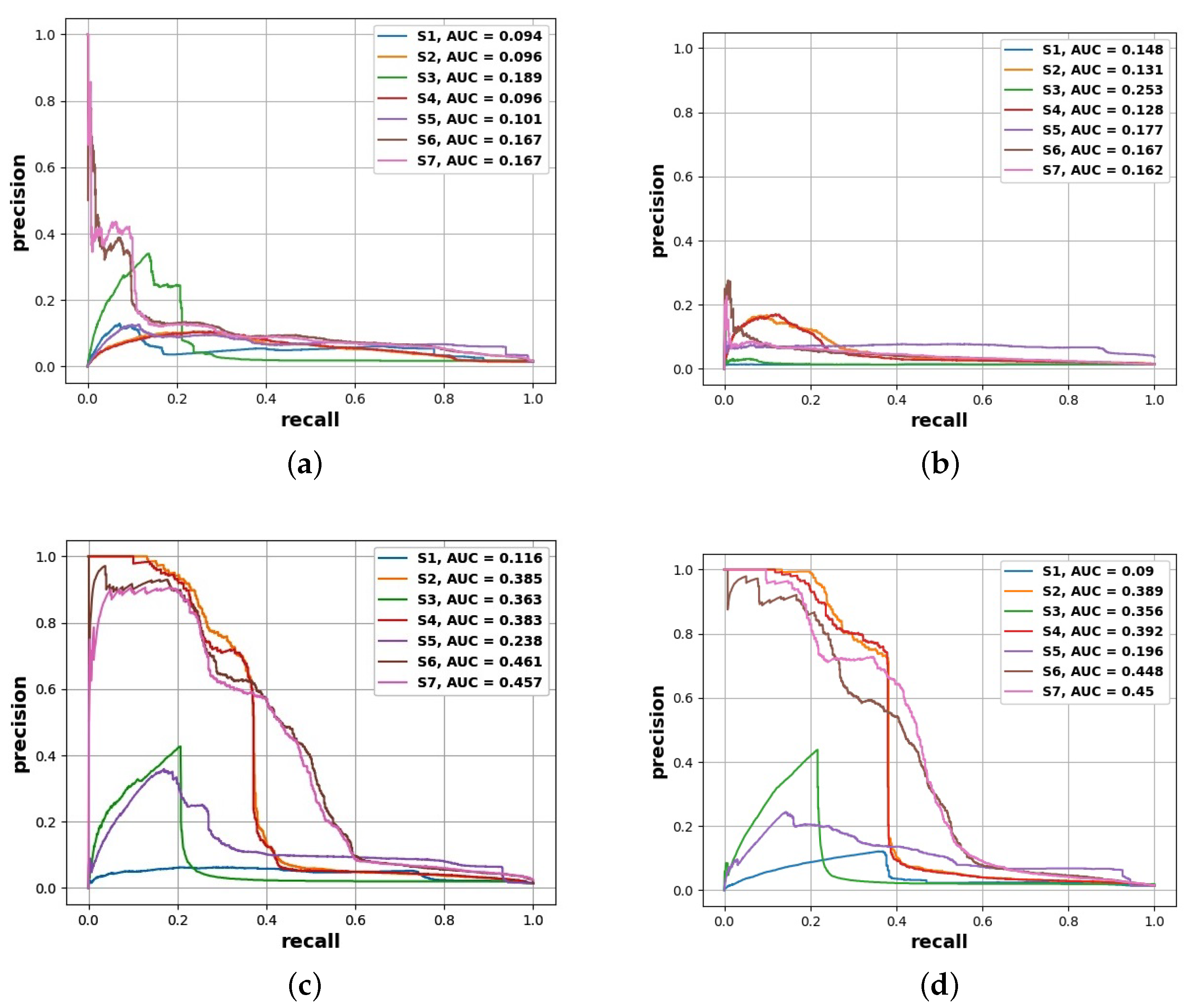
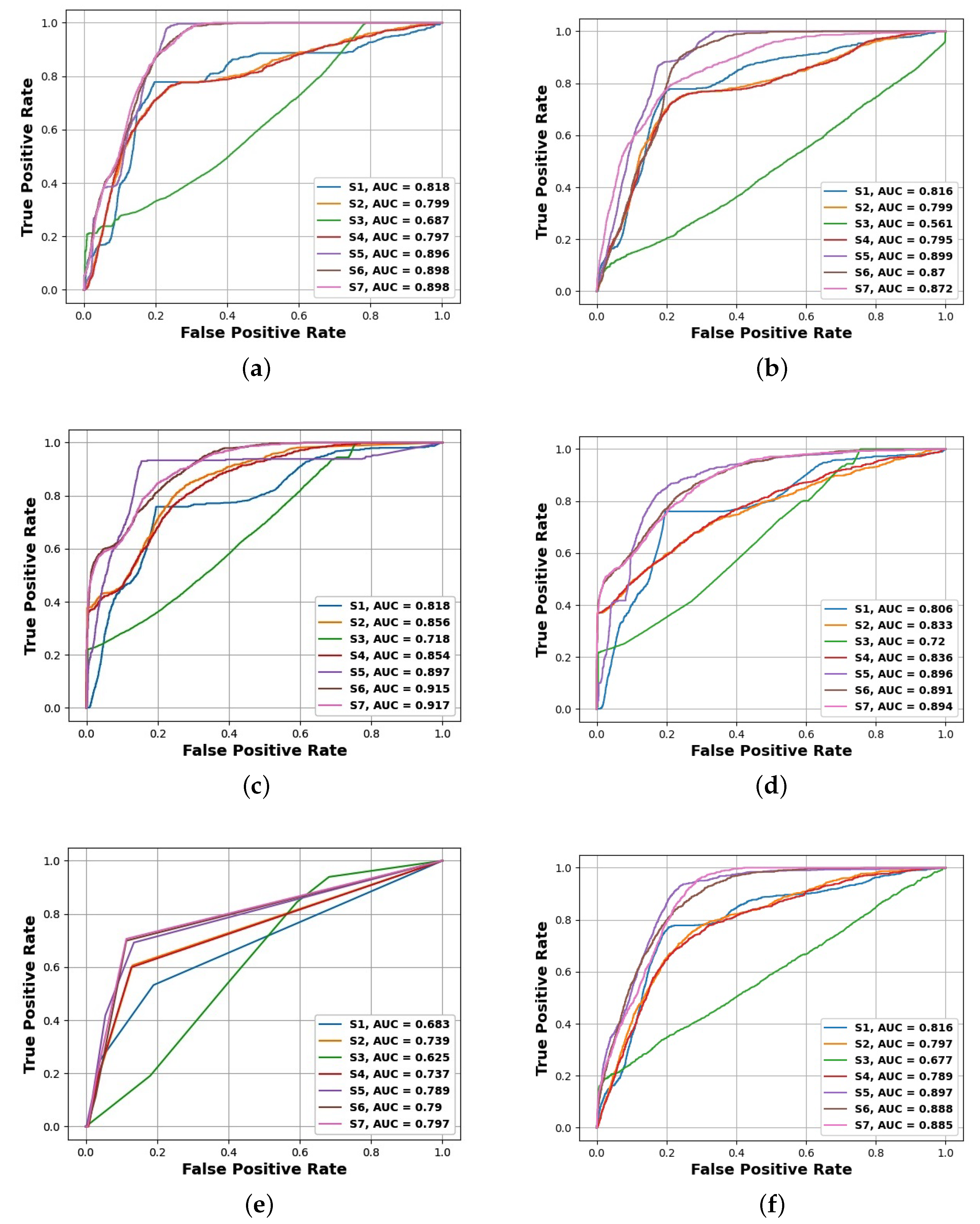
• The best prediction corresponds to a PR AUC of about $0.5$ and an ROC AUC of about $0.92$;
• Depending on the choice of cutoff thresholds, model, operating points are possibly achieving the true-positive rate of more than $0.9$ with the false-positive rate below $0.2$ or both the recall and precision above $0.5$;
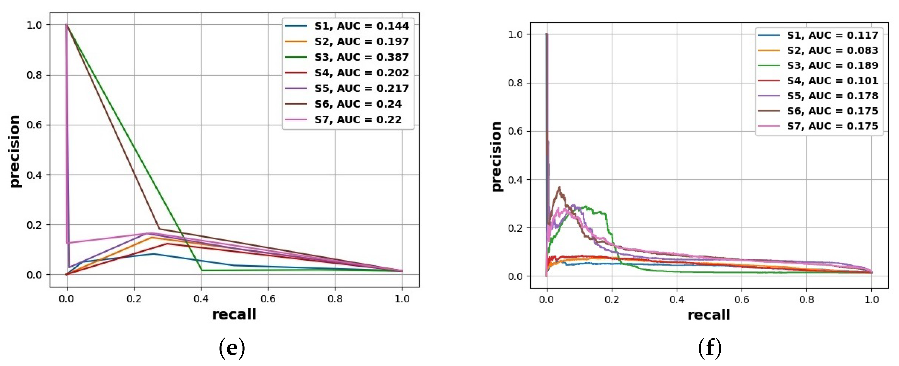
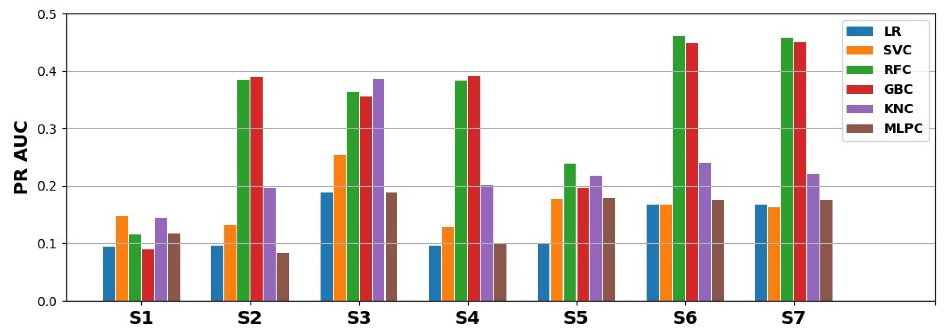
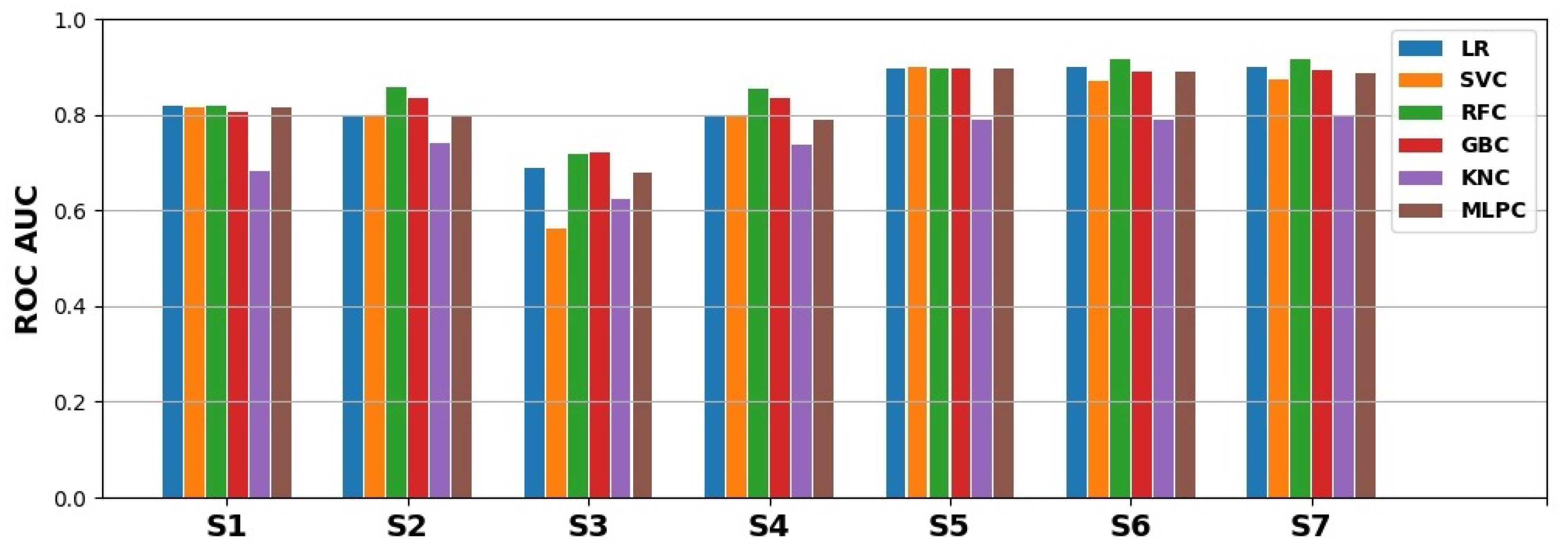
• PR curves and PR AUC values reveal more substantial predictive performance differences than do ROC curves and ROC AUC values, which is to be expected for heavily imbalanced data;
• The best models are obtained using the random forest and gradient boosting algorithms, which seem to deal best with the problems of small data size and class imbalance;
• Subsets $S6$ and $S7$ were found to be the most useful in the experiments carried out;
• The utility of smaller attribute subsets depends more on the adopted performance measure than on the algorithm, and in particular, attribute subsets $S1$ and $S5$ are the least useful with respect to PR AUC, while attribute subset $S3$ is the least useful with respect to ROC AUC.

It is not surprising that subsets S6 and S7 appear to have the largest impact for performance with respect to both ROC and PR since these subsets contain the largest number of attributes. Most intriguing, however, is the contribution of S3 subset, i.e., the attributes corresponding to transponder parameters. These attributes make it possible to achieve reasonably good performance with respect to the area under the precision-recall curve, comparable to that of the S2 and S4 attribute sets, but the performance with respect to the area under the ROC curve is clearly inferior when compared with any other subset. Furthermore, it should be noted that the S4 attribute set that contains almost all attributes except those related to transponder parameters cannot outperform the S3 subset with respect to PR without adding transponder-related attributes. Thus, there is a significant improvement in performance resulting from including transponder parameters when considering PR. However, with respect to ROC the performance improvement resulting from transponder-related parameters appears to be only marginal (i.e., there is only a minor difference between ROC AUC values for the S4 and S7 subsets).

It is also worth noting that there is a significant difference in performance with respect to PR in the case of the S5 and S7 subsets, which is not mirrored in the ROC results. In the case of ROC, the most complete sets, i.e., S5, S6, and S7, show almost identical performance. However, for PR, this is not the case. Finally, we observed that the S1 subset, which is essentially only one parameter, leads to a surprisingly good performance in the case of ROC but not in the case of PR. This last case stresses again the fact that due to severe class imbalance, PR analysis is a much more reliable predictive performance evaluation method than is ROC analysis since ROC tends to give an overoptimistic picture. Accordingly, PR analysis provides more reliable observations regarding the predictive utility of different attribute subsets than does ROC analysis.

6. Conclusions

In summary, our study shows that with an appropriately adjusted cutoff threshold for class probability predictions, one can obtain operating points with both the precision and recall above $0.5$ or with a true-positive rate of more than $0.9$ and a false-positive rate of less than $0.2$. The best performance was obtained using the gradient boosting and random forest algorithms. Using these algorithms, the best level of predictive performance with the area under the precision-recall curve is about $0.5$ and the area under the ROC curve is about $0.92$.

The results presented in this article fill some gaps left by prior work and lay more solid grounds for future work. In particular, this extended study uses a broader set of state-of-the-art machine learning algorithms and more systematically evaluates the utility of different attribute subsets, corresponding to different properties of network paths and their components. For the best identified setups, the achieved level of the area under the precision-recall curve exceeds that reported previously [7]. Under severe class imbalance, this is the most reliable performance metric, and the obtained value of 0.5 indicates a more practically useful tradeoff between the capability to detect bad paths and the tendency to misdetect good paths as bad.

Despite the progress our study represents, there remains space for further improvements in future work. Promising directions include examining the possibility of trained model transfer between different networks and enhancing network path descriptions by using additional attributes derived from physical channel properties.

Encouraging results obtained with one-class classification algorithms [8,45] suggest that it may be possible to combine binary and one-class classifiers into an even more successful hybrid model. Each of these future research lines would definitely benefit from more data, covering a wider range of network topologies and equipment and with a more comprehensive representation of unsuccessful path designs.

References

1. Kozdrowski, S.; Żotkiewicz, M.; Sujecki, S. Ultra-Wideband WDM Optical Network Optimization. Photonics 2020, 7, 16. [Google Scholar] [CrossRef] [Green Version]
2. Klinkowski, M.; Żotkiewicz, M.; Walkowiak, K.; Pióro, M.; Ruiz, M.; Velasco, L. Solving large instances of the RSA problem in flexgrid elastic optical networks. IEEE/OSA J. Opt. Commun. Netw. 2016, 8, 320–330. [Google Scholar] [CrossRef] [Green Version]
3. Ruiz, M.; Pióro, M.; Żotkiewicz, M.; Klinkowski, M.; Velasco, L. Column generation algorithm for RSA problems in flexgrid optical networks. Photonic Netw. Commun. 2013, 26, 53–64. [Google Scholar] [CrossRef]
4. Dallaglio, M.; Giorgetti, A.; Sambo, N.; Velasco, L.; Castoldi, P. Routing, Spectrum, and Transponder Assignment in Elastic Optical Networks. J. Light. Technol. 2015, 33, 4648–4658. [Google Scholar] [CrossRef] [Green Version]
5. Kozdrowski, S.; Żotkiewicz, M.; Sujecki, S. Resource optimization in fully flexible optical node architectures. In Proceedings of the 20th International Conference on Transparent Optical Networks (ICTON), Bucharest, Romania, 1–5 July 2018. [Google Scholar]
6. Kozdrowski, S.; Żotkiewicz, M.; Sujecki, S. Optimization of Optical Networks Based on CDC-ROADM Tech. Appl. Sci. 2019, 9, 399. [Google Scholar] [CrossRef] [Green Version]
7. Kozdrowski, S.; Cichosz, P.; Paziewski, P.; Sujecki, S. Machine Learning Algorithms for Prediction of the Quality of Transmission in Optical Networks. Entropy 2021, 23, 7. [Google Scholar] [CrossRef]
8. Cichosz, P.; Kozdrowski, S.; Sujecki, S. Application of ML Algorithms for Prediction of the QoT in Optical Networks with Imbalanced and Incomplete Data. In Proceedings of the 2021 International Conference on Software, Telecommunications and Computer Networks (SoftCOM), Split, Croatia, 23–25 September 2021; pp. 1–6. [Google Scholar] [CrossRef]
9. Mestres, A.; Rodríguez-Natal, A.; Carner, J.; Barlet-Ros, P.; Alarcón, E.; Solé, M.; Muntés, V.; Meyer, D.; Barkai, S.; Hibbett, M.J.; et al. Knowledge-Defined Networking. arXiv 2016, arXiv:1606.06222. [Google Scholar] [CrossRef] [Green Version]
10. Żotkiewicz, M.; Szałyga, W.; Domaszewicz, J.; Bak, A.; Kopertowski, Z.; Kozdrowski, S. Artificial Intelligence Control Logic in Next-Generation Programmable Networks. Appl. Sci. 2021, 11, 9163. [Google Scholar] [CrossRef]
11. Morais, R.M.; Pedro, J. Machine learning models for estimating quality of transmission in DWDM networks. IEEE/OSA J. Opt. Commun. Netw. 2018, 10, D84–D99. [Google Scholar] [CrossRef]
12. Musumeci, F.; Rottondi, C.; Nag, A.; Macaluso, I.; Zibar, D.; Ruffini, M.; Tornatore, M. An Overview on Application of Machine Learning Techniques in Optical Networks. IEEE Commun. Surv. Tutor. 2019, 21, 1383–1408. [Google Scholar] [CrossRef] [Green Version]
13. Rottondi, C.; Barletta, L.; Giusti, A.; Tornatore, M. Machine-learning method for quality of transmission prediction of unestablished lightpaths. IEEE/OSA J. Opt. Commun. Netw. 2018, 10, A286–A297. [Google Scholar] [CrossRef] [Green Version]
14. Panayiotou, T.; Manousakis, K.; Chatzis, S.P.; Ellinas, G. A Data-Driven Bandwidth Allocation Framework With QoS Considerations for EONs. J. Light. Technol. 2019, 37, 1853–1864. [Google Scholar] [CrossRef]
15. Pan, X.; Wang, X.; Tian, B.; Wang, C.; Zhang, H.; Guizani, M. Machine-Learning-Aided Optical Fiber Communication System. IEEE Netw. 2021, 35, 136–142. [Google Scholar] [CrossRef]
16. Lu, J.; Fan, Q.; Zhou, G.; Lu, L.; Yu, C.; Lau, A.P.T.; Lu, C. Automated training dataset collection system design for machine learning application in optical networks: An example of quality of transmission estimation. J. Opt. Commun. Netw. 2021, 13, 289–300. [Google Scholar] [CrossRef]
17. Zhou, Y.; Yang, Z.; Sun, Q.; Yu, C.; Yu, C. An artificial intelligence model based on multi-step feature engineering and deep attention network for optical network performance monitoring. Optik 2023, 273, 170443. [Google Scholar] [CrossRef]
18. Memon, K.A.; Butt, R.A.; Mohammadani, K.H.; Das, B.; Ullah, S.; Memon, S.; ul Ain, N. A Bibliometric Analysis and Visualization of Passive Optical Network Research in the Last Decade. Opt. Switch. Netw. 2020, 39, 100586. [Google Scholar] [CrossRef]
19. Ali, K.; Zhang, Q.; Butt, R.; Mohammadani, K.; Faheem, M.; Ain, N.; Feng, T.; Xin, X. Traffic-Adaptive Inter Wavelength Load Balancing for TWDM PON. IEEE Photonics J. 2020, 12, 7200408. [Google Scholar] [CrossRef]
20. Mata, J.; de Miguel, I.; Durán, R.J.; Aguado, J.C.; Merayo, N.; Ruiz, L.; Fernández, P.; Lorenzo, R.M.; Abril, E.J. A SVM approach for lightpath QoT estimation in optical transport networks. In Proceedings of the 2017 IEEE International Conference on Big Data (Big Data), Boston, MA, USA, 11–14 December 2017; pp. 4795–4797. [Google Scholar]
21. Thrane, J.; Wass, J.; Piels, M.; Medeiros Diniz, J.; Jones, R.; Zibar, D. Machine Learning Techniques for Optical Performance Monitoring from Directly Detected PDM-QAM Signals. J. Light. Technol. 2017, 35, 868–875. [Google Scholar] [CrossRef] [Green Version]
22. Barletta, L.; Giusti, A.; Rottondi, C.; Tornatore, M. QoT estimation for unestablished lighpaths using machine learning. In Proceedings of the 2017 Optical Fiber Communications Conference and Exhibition (OFC), Los Angeles, CA, USA, 19–23 March 2017; pp. 1–3. [Google Scholar]
23. Seve, E.; Pesic, J.; Delezoide, C.; Bigo, S.; Pointurier, Y. Learning Process for Reducing Uncertainties on Network Parameters and Design Margins. J. Optital Commun. Netw. 2018, 10, A298–A306. [Google Scholar] [CrossRef]
24. Japkowicz, N. Learning from Imbalanced Data Sets: A Comparison of Various Strategies; AAAI Press: Menlo Park, CA, USA, 2000. [Google Scholar]
25. Bellinger, C.; Sharma, S.; Zaïane, O.R.; Japkowicz, N. Sampling a Longer Life: Binary versus One-Class Classification Revisited. Proc. Mach. Learn. Res. 2017, 74, 64–78. [Google Scholar]
26. Lee, H.; Cho, S. The Novelty Detection Approach for Different Degrees of Class Imbalance. In Proceedings of the 13th International Conference on Neural Information Processing, ICONIP-2006, Hong Kong, China, 3–6 October 2006; Springer: Berlin/Heidelberg, Germany, 2006. [Google Scholar]
27. Chawla, N.V.; Bowyer, K.W.; Hall, L.O.; Kegelmeyer, W.P. SMOTE: Synthetic Minority Over-sampling Technique. J. Artif. Intell. Res. 2002, 16, 321–357. [Google Scholar] [CrossRef]
28. Menardi, G.; Torelli, N. Training and Assessing Classification Rules with Imbalanced Data. Data Min. Knowl. Discov. 2014, 28, 92–122. [Google Scholar] [CrossRef]
29. Mo, W.; Huang, Y.K.; Zhang, S.; Ip, E.; Kilper, D.C.; Aono, Y.; Tajima, T. ANN-Based Transfer Learning for QoT Prediction in Real-Time Mixed Line-Rate Systems. In Proceedings of the Optical Fiber Communication Conference, San Diego, CA, USA, 11–15 March 2018; Optica Publishing Group: Massachusetts, NW, USA, 2018; p. 4. [Google Scholar]
30. Proietti, R.; Chen, X.; Castro, A.; Liu, G.; Lu, H.; Zhang, K.; Guo, J.; Zhu, Z.; Velasco, L.; Yoo, S.J.B. Experimental Demonstration of Cognitive Provisioning and Alien Wavelength Monitoring in Multi-domain EON. In 2018 Optical Fiber Communications Conference and Exposition (OFC); Optical Society of America: Washington, DC, USA, 2018; pp. 1–3. [Google Scholar]
31. Hilbe, J.M. Logistic Regression Models; Chapman and Hall: London, UK, 2009. [Google Scholar]
32. Cortes, C.; Vapnik, V.N. Support-Vector Networks. Mach. Learn. 1995, 20, 273–297. [Google Scholar] [CrossRef]
33. Platt, J.C. Fast Training of Support Vector Machines using Sequential Minimal Optimization. In Advances in Kernel Methods: Support Vector Learning; Schölkopf, B., Burges, C.J.C., Smola, A.J., Eds.; MIT Press: Cambridge, MA, USA, 1998. [Google Scholar]
34. Hamel, L.H. Knowledge Discovery with Support Vector Machines; Wiley: Hoboken, NJ, USA, 2009. [Google Scholar]
35. Platt, J.C. Probabilistic Outputs for Support Vector Machines and Comparison to Regularized Likelihood Methods. In Advances in Large Margin Classifiers; Smola, A.J., Barlett, P., Schölkopf, B., Schuurmans, D., Eds.; MIT Press: Cambridge, MA, USA, 2000. [Google Scholar]
36. Breiman, L. Random Forests. Mach. Learn. 2001, 45, 5–32. [Google Scholar] [CrossRef] [Green Version]
37. Strobl, C.; Boulesteix, A.L.; Zeileis, A.; Hothorn, T. Bias in Random Forest Variable Importance Measures: Illustrations, Sources and a Solution. BMC Bioinform. 2007, 8, 25. [Google Scholar] [CrossRef] [Green Version]
38. Schapire, R.E. The Strength of Weak Learnability. Mach. Learn. 1990, 5, 197–227. [Google Scholar] [CrossRef] [Green Version]
39. Schapire, R.E.; Freund, Y. Boosting: Foundations and Algorithms; MIT Press: Cambridge, MA, USA, 2012. [Google Scholar]
40. Ke, G.; Meng, Q.; Finley, T.; Wang, T.; Chen, W.; Ma, W.; Ye, Q.; Liu, T.Y. LightGBM: A Highly Efficient Gradient Boosting Decision Tree. In Proceedings of the Advances in Neural Information Processing Systems 30 (NeurIPS-2017), Long Beach, CA, USA, 4–9 December 2017. [Google Scholar]
41. Cover, T.M.; Hart, P.E. Nearest Neighbor Pattern Classification. IEEE Trans. Inf. Theory 1967, 13, 21–27. [Google Scholar] [CrossRef] [Green Version]
42. Hinton, G.E. Connectionist Learning Procedures. Artif. Intell. 1989, 40, 185–234. [Google Scholar] [CrossRef] [Green Version]
43. Glorot, X.; Bordes, A.; Bengio, Y. Deep Sparse Rectifier Neural Networks. In Proceedings of the 14th International Conference on Artificial Intelligence and Statistics (AISTATS-2011), Fort Lauderdale, FL, USA, 11–13 April 2011. [Google Scholar]
44. Pedregosa, F.; Varoquaux, G.; Gramfort, A.; Michel, V.; Thirion, B.; Grisel, O.; Blondel, M.; Prettenhofer, P.; Weiss, R.; Dubourg, V.; et al. Scikit-learn: Machine Learning in Python. J. Mach. Learn. Res. 2011, 12, 2825–2830. [Google Scholar]
45. Cichosz, P.; Kozdrowski, S.; Sujecki, S. Learning to Classify DWDM Optical Channels from Tiny and Imbalanced Data. Entropy 2021, 23, 1504. [Google Scholar] [CrossRef]
Figure 1. Data preparation process.
Applsci 13 04657 g001
Figure 2. An example of optical network topology.
Applsci 13 04657 g002
Figure 3. Network subsection illustrating the meaning of the specific channel attributes occurring in the studied database.
Applsci 13 04657 g003
Figure 4. PR curves for particular algorithms and attribute subsets. (a) LR classifier; (b) SVC classifier; (c) RF classifier; (d) GB classifier; (e) KN classifier; (f) MLP classifier.
Applsci 13 04657 g004aApplsci 13 04657 g004b
Figure 5. ROC curves for particular algorithms and attribute subsets. (a) LR classifier; (b) SVC classifier; (c) RF classifier; (d) GB classifier; (e) KN classifier; (f) MLP classifier.
Applsci 13 04657 g005
Figure 6. PR AUC values for particular algorithms and attribute subsets.
Applsci 13 04657 g006
Figure 7. ROC AUC values for particular algorithms and attribute subsets.
Applsci 13 04657 g007