Integrating Deep Learning and Deterministic Inversion for Enhancing Fault Detection in Electrical Resistivity Surveys

Abstract

Clays in fault zones have low electrical resistivity, making electrical resistivity tomography (ERT) effective for fault investigations. However, traditional ERT inversion methods struggle to find a unique solution and produce unstable results owing to the ill-posed nature of the problem. To address this, a workflow integrating deep-learning (DL) technology with traditional ERT inversion is proposed. First, a deep-learning model named DL-ERT inversion that maps apparent resistivity data to subsurface resistivity models is developed. To create target-oriented training data, we use approximately 150 field borehole data acquired from various survey areas in South Korea. The DL-ERT inversion algorithm is based on a U-Net structure and includes an additional network called the borehole mixer to incorporate borehole information when available. The DL-ERT inversion model is trained in three stages: base model training, borehole mixer training, and fine-tuning. Results showed that the fine-tuning model provided the highest prediction accuracy for all test datasets. Next, the prediction of the trained model is used as the initial model for the deterministic inversion method to predict the final subsurface model. The efficiency and accuracy of the proposed workflow are demonstrated in fault detection using a field data example compared with traditional deterministic inversion.

1. Introduction

Faults are typically characterized by soft ground as rocks become fractured and clays and groundwater are introduced due to repeated movements over time. Therefore, faults are considered a crucial aspect in investigations of site characteristics for large-scale construction, such as geological surveys, tunnels, and bridges, as well as in ground stability assessment, including ground subsidence, tunnel collapse, and slope stability investigations [1,2,3]. Geophysical exploration techniques, including seismic, electrical, and electromagnetic methods, are actively being used in various fields to detect faults [4,5,6,7,8,9]. In particular, fault zones, weathered zones, and aquifers containing clay minerals exhibit low electrical resistivity, making electrical resistivity tomography (ERT) surveys an effective tool in fault zone investigations [10].

Numerous studies have been dedicated to the detection and characterization of fault zones using electrical resistivity surveys. Rønning et al. [11] investigated the application of resistivity mapping in identifying and characterizing weakness zones in crystalline bedrock, providing a valuable tool for assessing rock stability and geological engineering. Ganerød et al. [12] conducted a comparative analysis of different geophysical methods and determined resistivity measurement to be the most effective technique for mapping faults and fracture zones. Moreover, extensive research has been conducted on fault detection by utilizing electrical resistivity surveys in both terrestrial and marine environments [13,14,15,16,17]. These studies collectively demonstrate the wide-ranging applicability and effectiveness of electrical resistivity surveys in detecting and mapping fault structures.

To analyze fault zones in electrical resistivity surveys, deterministic inversion methods are typically used. However, the traditional inversion process is challenging due to its ill-posed nature, which can result in non-unique and unstable solutions. In particular, if the initial model is far from the true subsurface properties, it can lead to convergence problems or inaccurate estimates. Additionally, the complexity of the numerical calculations involved makes the inversion process both time-consuming and computationally expensive [18,19].

Recently, studies have actively incorporated deep-learning technology into ERT inversion to overcome its limitations. Liu et al. [20] introduced ERSInvNet, which is based on the U-Net architecture, for mapping apparent resistivity data to resistivity models. They used a tier feature map as an additional input feature to mitigate the ambiguity that arises when using a convolutional neural network (CNN) due to the vertical variation in patterns between the input and output. Liu et al. [21] also designed an adaptive CNN for electrical resistivity inversion, taking into account the vertically varying characteristics between apparent resistivity data and resistivity models. Similarly, Vu and Jardani [22] proposed a deep-learning algorithm for the three-dimensional (3D) reconstruction of ERT, using SegNet architecture for the inversion network and training it with subsurface resistivity models generated by a geostatistical anisotropic Gaussian generator and corresponding apparent resistivity. Wilson et al. [23] also developed a ERT inversion using deep learning, proposing a variational encoder–decoder network for the inversion network and constructing realistic resistivity synthetic models with complex layers. Furthermore, various studies have applied similar approaches to electromagnetic (EM) inversion, with Oh et al. [24] developing a CNN model to delineate salt dome structure from marine controlled-source EM (CSEM) data and other studies utilizing deep-learning technology for the inversion of airborne EM data [25,26,27].

Although these methods have shown promising results, their training datasets were not target-oriented; rather, they aimed to achieve a general solution by creating subsurface models with randomly selected box-shaped anomalies or multiple layers. However, because the inverse problem is ill-posed in nature, a deep-learning approach still requires constraints, such as regularization terms in traditional inversion, to ensure the stability and reliability of the solution. In the deep-learning approach, these constraints can be incorporated when generating training data by adding prior knowledge, such as information about background layers obtained from borehole data in the application area. Additionally, these methods do not incorporate borehole data, which can be utilized to improve the inversion results when available. Furthermore, although the deep-learning model is well-trained using a training dataset that closely resembles realistic settings, the trained model is not guaranteed to obtain the optimal solution because the distribution of the target field data may differ from that of the training data.

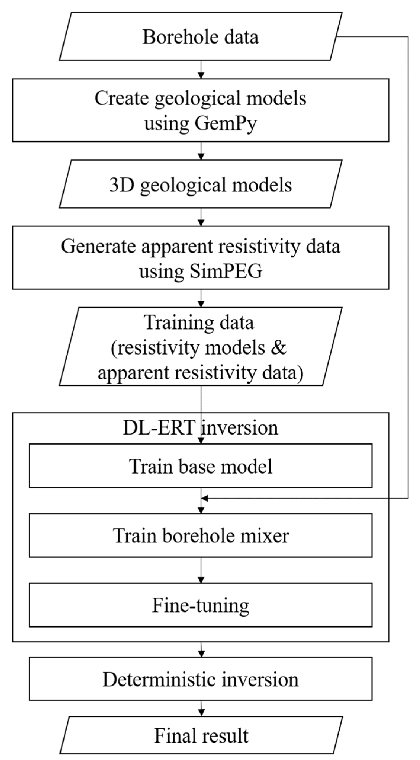
To address the abovementioned limitations, we propose a new workflow that combines deep-learning technology with traditional deterministic inversion to enhance fault detection in electrical resistivity surveys. First, we create a target-oriented training dataset for fault detection using field borehole data. Then, we develop a deep-learning model based on the U-Net architecture using the training dataset for ERT inversion. In addition, we include an additional network called borehole mixer at the end of the U-Net, which incorporates borehole information to enhance the inversion results if borehole data are available. Finally, we use the prediction of the trained model as the initial subsurface model for deterministic inversion to predict the final subsurface model. Through numerical examples of synthetic and field data, we have obtained encouraging experimental results, which indicate that the proposed workflow has better performance than the traditional inversion in fault detection.

2. Methodology

In this section, we first explain to the procedure for creating geological models based on field borehole data and corresponding apparent resistivity data using the open-source libraries GemPy and SimPEG, respectively. Then, we illustrate the network structure and training process of the deep learning-based ERT inversion, called DL-ERT inversion. Finally, we propose an approach to integrate DL-ERT inversion with deterministic inversion using the prediction of DL-ERT inversion as the initial model for the deterministic inversion. Figure 1 shows the flowchart of the proposed workflow.

2.1. Creating Target-Oriented Resistivity Models Based on Field Borehole Data Using GemPy

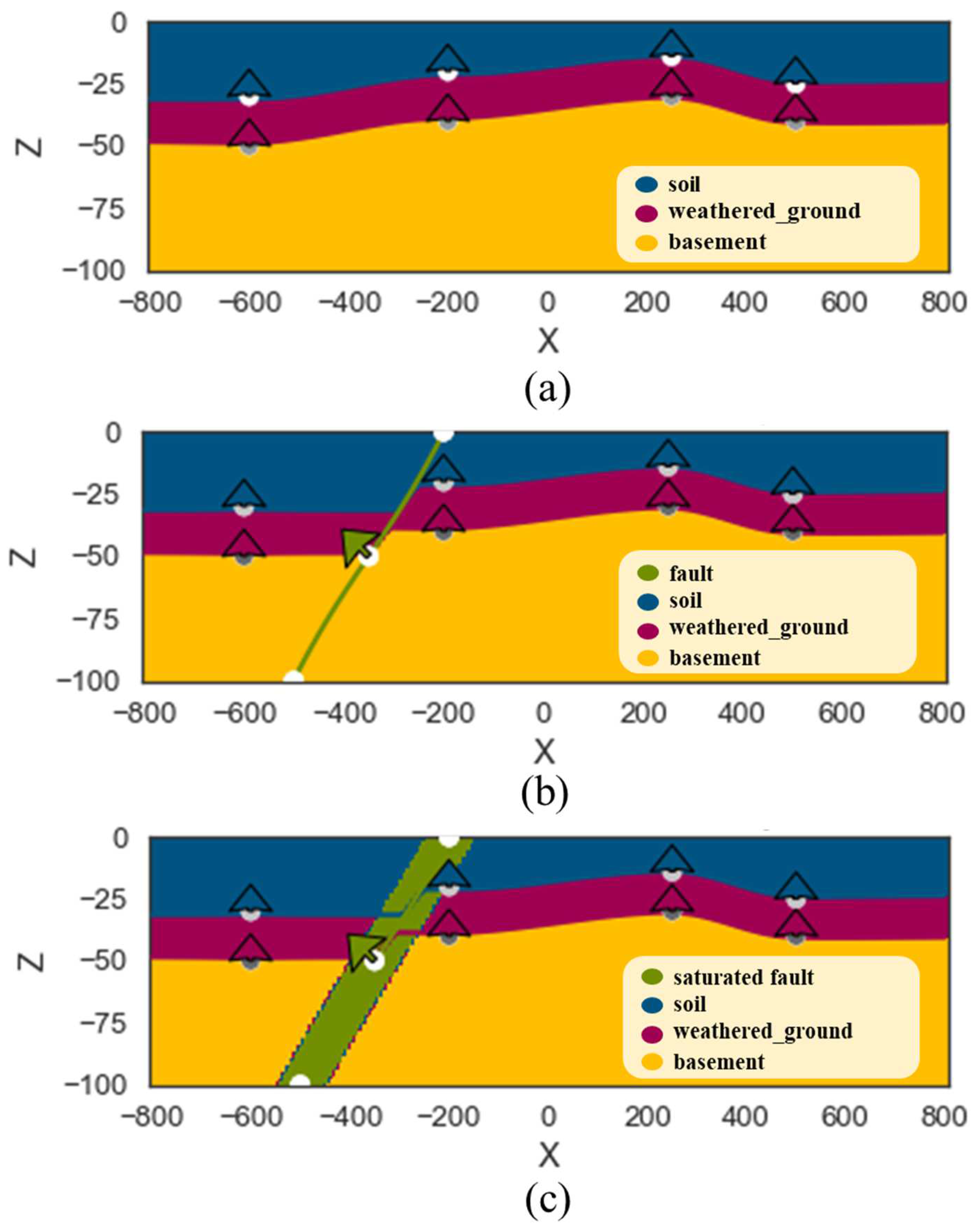
To create a deep-learning model optimized for fault zone detection, we employed a method that involved generating subsurface resistivity models based on field borehole data using GemPy, an open-source Python library for 3D geological modeling [28]. The potential-field method developed by Lajaunie [29] was used to create a 3D geological model in GemPy. To create a stratigraphic model, it is important to interpolate lithological interfaces that show changes in physical properties using a scalar field value [30]. The input values for the scalar field include layer interface points that represent interfaces between two layers and gradients of the scalar field that indicate poles of the layer. The layer interface points are also known as surface contact points, and the gradients of the scalar field are referred to as orientations. The scalar values are subsequently calculated for all interfaces in the scalar field to identify the lithology of every point in the mesh. By discretizing 3D space, we generated a layered model, as shown in Figure 2a, which is a vertical section of the 3D model.

To create a fault structure, we added surface contact points and orientations for a fault to the layered model, as depicted in Figure 2b. To simulate the assumption that the fault zone is saturated with groundwater, we increased the thickness of the existing fault line, which resulted in the saturated fault structure shown in Figure 2c.

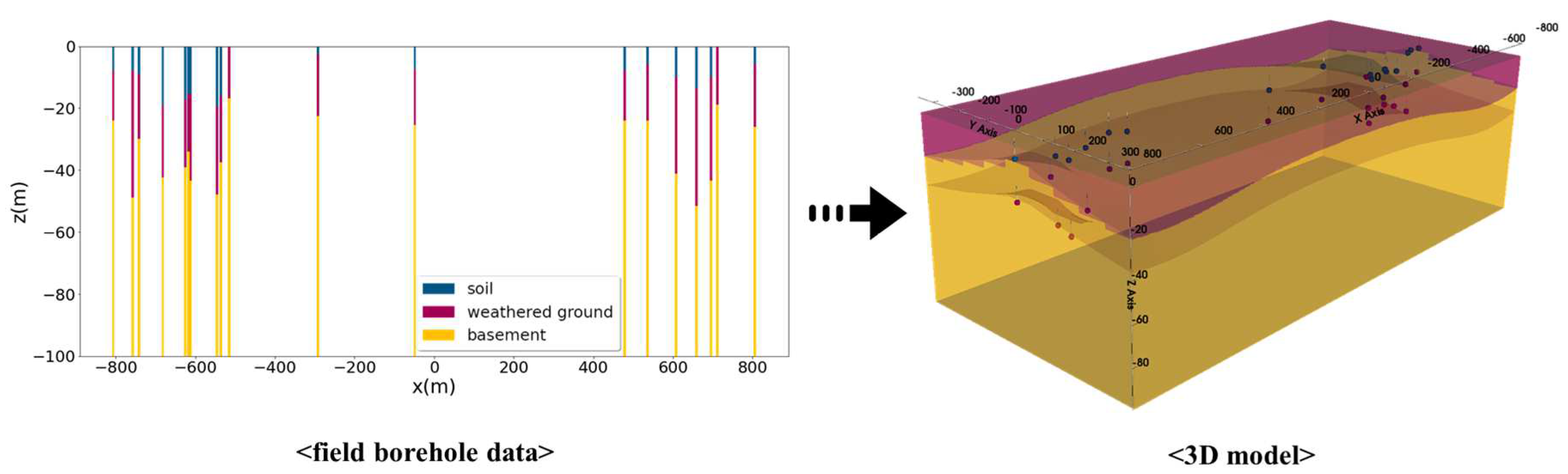
In this work, field borehole data and resistivity properties were used to create 3D resistivity models in GemPy. We assigned the same coordinates as the field borehole data and set the depths of each stratum as surface contact points with upward-facing surface orientations. This approach allowed us to generate realistic 3D layered models reflecting field conditions, as shown in Figure 3. Additionally, to create a fault structure, the surface points and displacements for the faults were assigned randomly, and the surface orientations were set close to perpendicular to the fault plane. Assuming the fault zone to be saturated with groundwater, a fault structure with a random thickness and low resistivity was created. From the 3D models, we randomly selected two-dimensional (2D) sections along survey lines to generate 2D resistivity models.

2.2. Generating Synthetic Apparent Resistivity Data Using SimPEG

Two-dimensional electrical resistivity forward modeling was performed to generate the apparent resistivity data using SimPEG, which is an open-source Python library for simulation and inversion of geophysical data [31]. In SimPEG, the DC resistivity forward modeling involves solving the governing equations given by:

$$\nabla ·\left(-\mathsf{\sigma }\nabla \mathsf{\varphi }\right)=I\left(\delta \left(\overrightarrow{r}-{\overrightarrow{r}}_A\right)-\delta \left(\overrightarrow{r}-{\overrightarrow{r}}_{\mathrm{B}}\right)\right),$$

(1)

where $\mathsf{\sigma }$ represents the electrical conductivity, $\mathsf{\varphi }$ represents the electrical potential, and $I$ is the input current at the positive and negative dipole locations, ${\overrightarrow{r}}_A$ and ${\overrightarrow{r}}_B$, respectively.

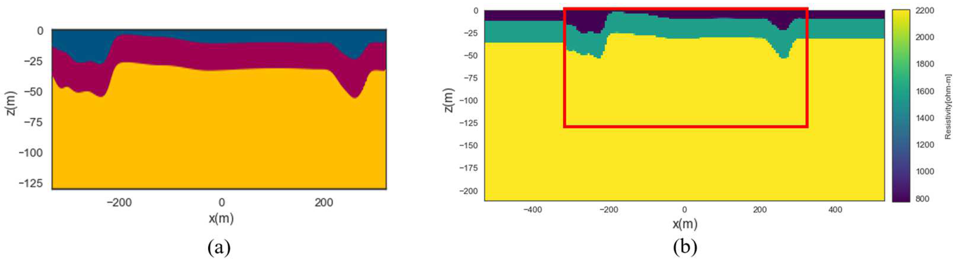
To simulate the partial differential Equation (1), the subsurface model was first discretized on a computational mesh. The conductivity values and potentials were then defined at the cell centers and nodes of the staggered grid, respectively. SimPEG provides several mesh options; in this study, a tensor mesh was used. The 2D resistivity sections generated from GemPy were interpolated onto the tensor mesh in SimPEG, and additional cells were added horizontally and vertically to ensure adequate satisfaction of the boundary conditions, as shown in Figure 4. The interpolated domain of the resistivity model, indicated by the red box in Figure 4b, served as a label (ground truth) for our deep-learning network in the inverse problem.

After Equation (1) was numerically solved, the potential fields were projected onto the receiver electrode locations through interpolation. The apparent resistivity (${\mathsf{\rho }}_{\mathrm{a}},$ ohm-m) could then be calculated using the following formula:

$${\mathsf{\rho }}_{\mathrm{a}}=\frac{{\mathsf{\Delta }\mathrm{V}}_{MN}}{I}\cdot \mathrm{K},$$

(2)

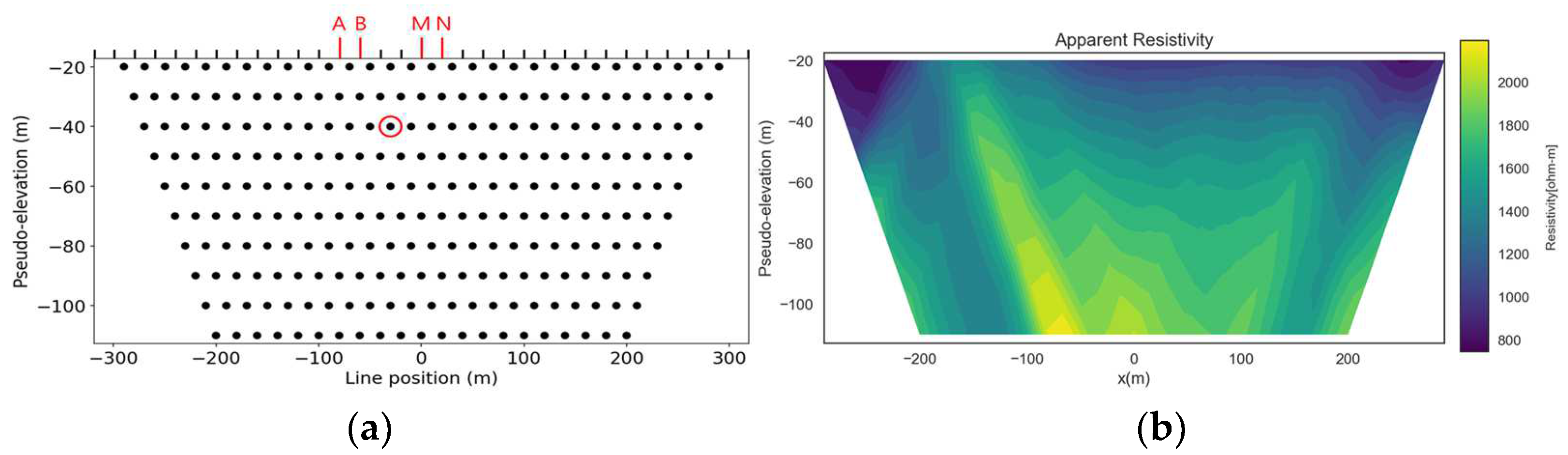
where ${\mathsf{\Delta }\mathrm{V}}_{MN}$(Volt) is the potential difference between two electrodes M and N; I is the electric current; K (m) is a geometric factor that depends on the geometry of the electrode array. K can be calculated as

$$\mathrm{K} =2\mathsf{\pi }\left[{\left(\frac{1}{\mathrm{AM}}-\frac{1}{\mathrm{MB}}-\frac{1}{\mathrm{AN}}+\frac{1}{\mathrm{NB}}\right)}^{-1}\right],$$

(3)

where A and B indicate the locations of the current electrodes; M and N indicate the locations of the potential electrodes in Figure 5a. In this study, a dipole–dipole array was used, and Figure 5b shows a pseudosection of the apparent resistivity, which was used as input for our deep-learning network for the inverse problem.

2.3. DL-ERT Inversion

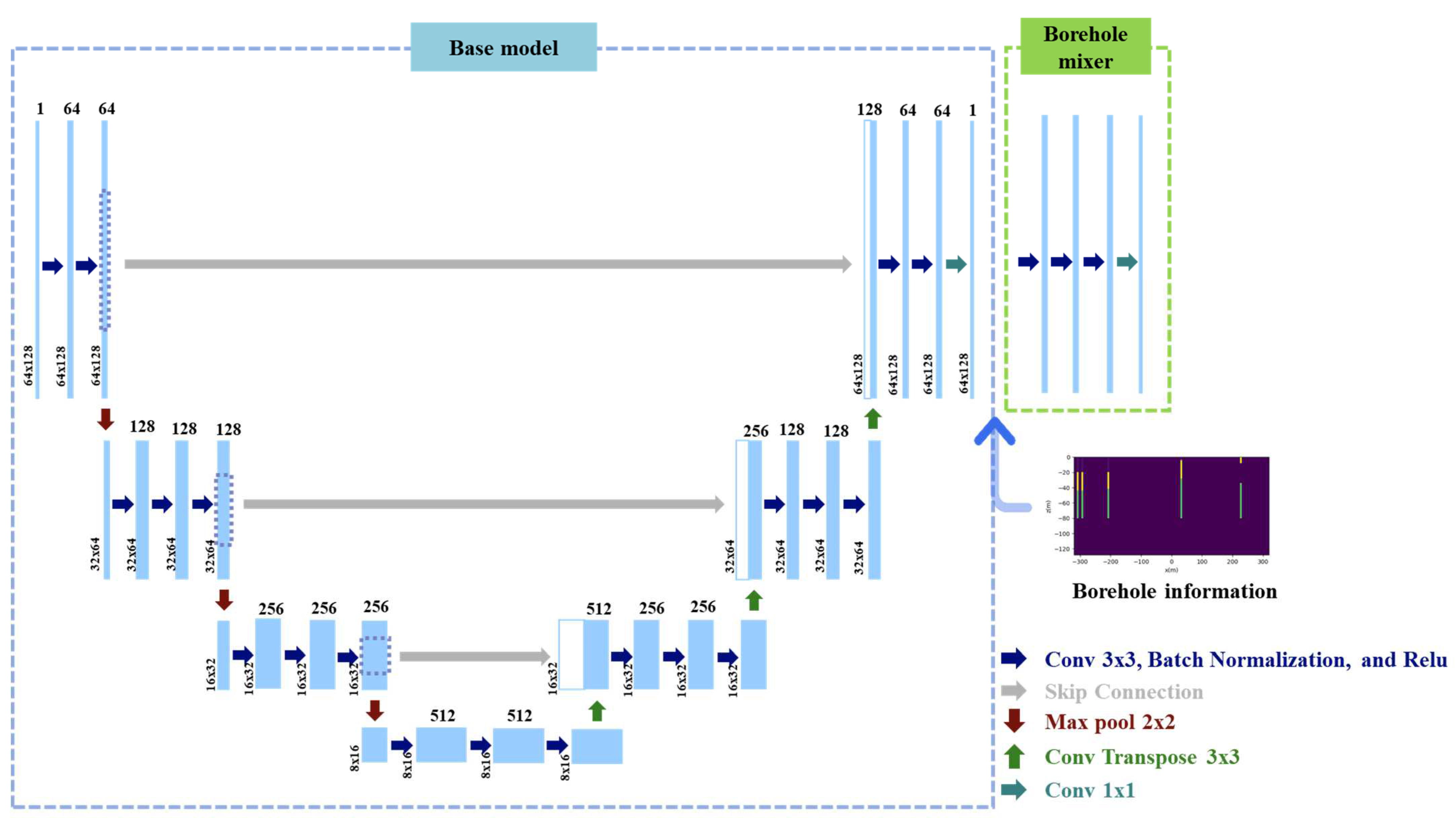
The deep-learning network for electrical resistivity tomography (DL-ERT) inversion comprised a base model and a borehole mixer. The base model was designed to perform pure ERT inversion using apparent resistivity data, $\mathit{d}$, for the direct estimation of the resistivity model, m, as follows:

$$\widehat{\mathit{m}}=Base\left(\mathit{d};\theta \right),$$

(4)

where $\theta$ denotes the model parameters of the base network, Base(), and $\widehat{\mathit{m}}$ is the predicted resistivity model of the base network. Note that the base model does not require borehole information. As illustrated in Figure 6, the base model employs a modified U-Net structure, which is a simplified version of the existing U-Net [32]. The inputs $\mathit{d}$ and labels m of this network are pseudosections of apparent resistivity and the corresponding 2D resistivity models, respectively, each having a size of 64 × 128. In the encoding path of the base model, the first convolution block is composed of two 3 × 3 convolutional layers and one 2 × 2 max-pooling layer. Other convolution blocks comprise three 3 × 3 kernel-size convolutional layers and one 2 × 2 kernel-size max-pooling layer. Batch normalization is applied after each convolutional layer to increase the learning speed and stabilize the learning process [33]. The rectified linear unit (ReLU) activation functions [34] are added for the convolutional layers. The decoder is symmetrical to the encoder, and the transposed convolutional layers are used to perform up-sampling in the decoding path [35]. Skip connections are used to prevent the loss of data information by directly connecting the encoder layer to the decoder layer. The detailed structure of the base model is presented in

Table 1. Base model structure.

Layer	Output Shape
Input_1	(64,128,1)
Conv2d	(64,128,64)
Conv2d_1	(64,128,64)
Max_pooling2d	(32,64,64)
Conv2d_2	(32,64,128)
Conv2d_3	(32,64,128)
Conv2d_4	(32,64,128)
Max_pooling2d_1	(16,32,128)
Conv2d_5	(16,32,256)
Conv2d_6	(16,32,256)
Conv2d_7	(16,32,256)
Max_pooling2d_2	(8,16,256)
Conv2d_8	(8,16,512)
Con2d_9	(8,16,512)
Conv2d_10	(8,16,512)
Conv2d_transpose	(16,32,256)
Concatenate	(16,32,512)
Conv2d_11	(16,32,256)
Conv2d_12	(16,32,256)
Conv2d_13	(16,32,256)
Conv2d_transpose_1	(32,64,128)
Concatenate_1	(32,64,256)
Conv2d_14	(32,64,128)
Conv2d_15	(32,64,128)
Conv2d_16	(32,64,128)
Conv2d_transpose_2	(64,128,64)
Concatenate_2	(64,128,128)
Conv2d_17	(64,128,64)
Conv2d_18	(64,128,64)
Conv2d_19	(64,128,1)

.

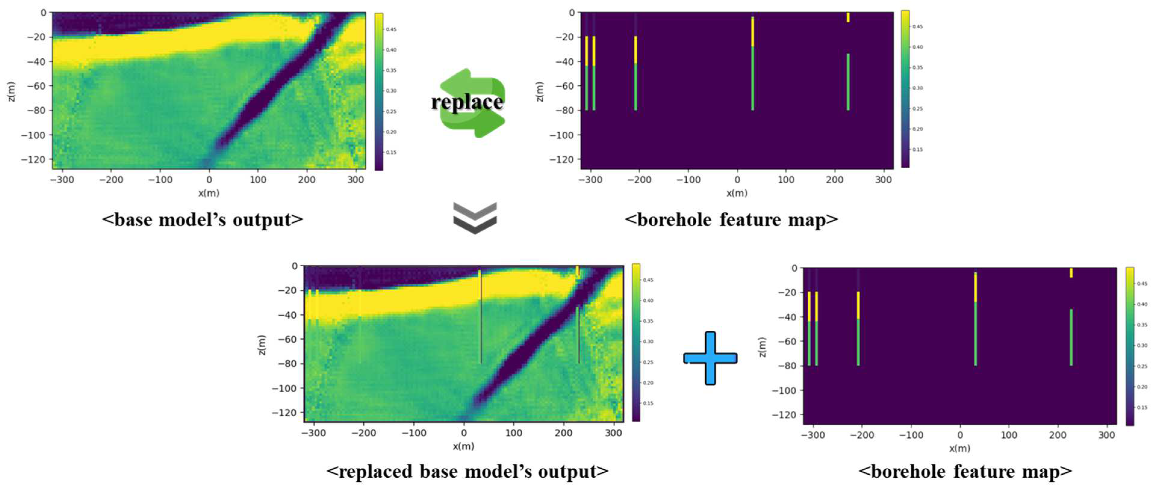
The borehole mixer is designed to incorporate borehole information into the network to improve the inversion results. A borehole feature map, b, is created by adding the true resistivity values at the borehole locations to a map of the same size as the output of the base model, $\widehat{\mathit{m}}$, setting all other parts except the borehole locations to zero, as shown in Figure 7. Then, the resistivity values of the output of the base model, $\widehat{\mathit{m}}$, are replaced with the true resistivity values of the borehole, and the replaced output and the borehole feature map, b, are concatenated and fed into the borehole mixer network. The following relationship can be employed for the final estimation of m:

$${\widehat{\mathit{m}}}^{*}=\mathrm{Mixer}\left(\widehat{\mathit{m}},\mathit{b};{\theta }^{*}\right),$$

(5)

where ${\theta }^{*}$ denotes the model parameters of the borehole mixer network, $\mathrm{Mixer}$(). The borehole mixer network is added to the output layer of the base model as shown in Figure 6, and the network is simply composed of four convolutional layers: three 13 × 13 convolutional layers and one 1 × 1 convolutional layer. The detailed structure of the borehole mixer network is presented in

Table 2. Borehole mixer network structure.

Layer	Output Shape
Concatenate	(64,128,2)
Conv2d	(64,128,64)
Conv2d_1	(64,128,64)
Conv2d_2	(64,128,64)
Conv2d_3	(64,128,1)

.

2.4. Network Training Strategy

The training process of the DL-ERT inversion network involves three stages: base model training, borehole mixer training, and fine-tuning. The base model is designed for mapping apparent resistivity to a resistivity model without using borehole information. Thus, the optimization problem of the base model training can be defined as follows:

$$\widehat{\theta }= \arg \underset{\theta }{\min }\frac{1}{N}{\displaystyle \sum }_{i=1}^N{\left({\mathit{m}}_i-\mathrm{Base}\left(\mathit{d};\theta \right)\right)}^2,$$

(6)

where N is the number of data.

In the borehole mixer training, the pre-trained model parameters of the base model, $\widehat{\theta }$, are transferred and frozen, and only the borehole mixer network is trained as follows:

$${\widehat{\theta }}^{*}=\arg \underset{{\theta }^{*}}{\min }\frac{1}{N}{\displaystyle \sum }_{i=1}^N{\left({\mathit{m}}_i-\mathrm{Mixer}\left(\widehat{\mathit{m}},\mathit{b};{\theta }^{*}\right)\right)}^2.$$

(7)

Finally, in the fine-tuning stage, the pre-trained base model and borehole mixer are unfrozen and re-trained to slightly adjust the inversion result:

$${\widehat{\theta }}_{final}=\arg \underset{\widehat{\theta }, {\widehat{\theta }}^{*}}{\min }\frac{1}{N}{\displaystyle \sum }_{i=1}^N{\left({\mathit{m}}_i-\mathrm{Base}\left(\mathit{d};\widehat{\theta }\right)\right)}^2+\frac{1}{N}{\displaystyle \sum }_{i=1}^N{\left({\mathit{m}}_i-\mathrm{Mixer}\left(\widehat{\mathit{m}},\mathit{b};{\widehat{\theta }}^{*}\right)\right)}^2$$

(8)

We solved Equations (6)–(8) using the Adam optimizer and set the learning rate to decrease at each stage for stable training with transfer learning and fine-tuning.

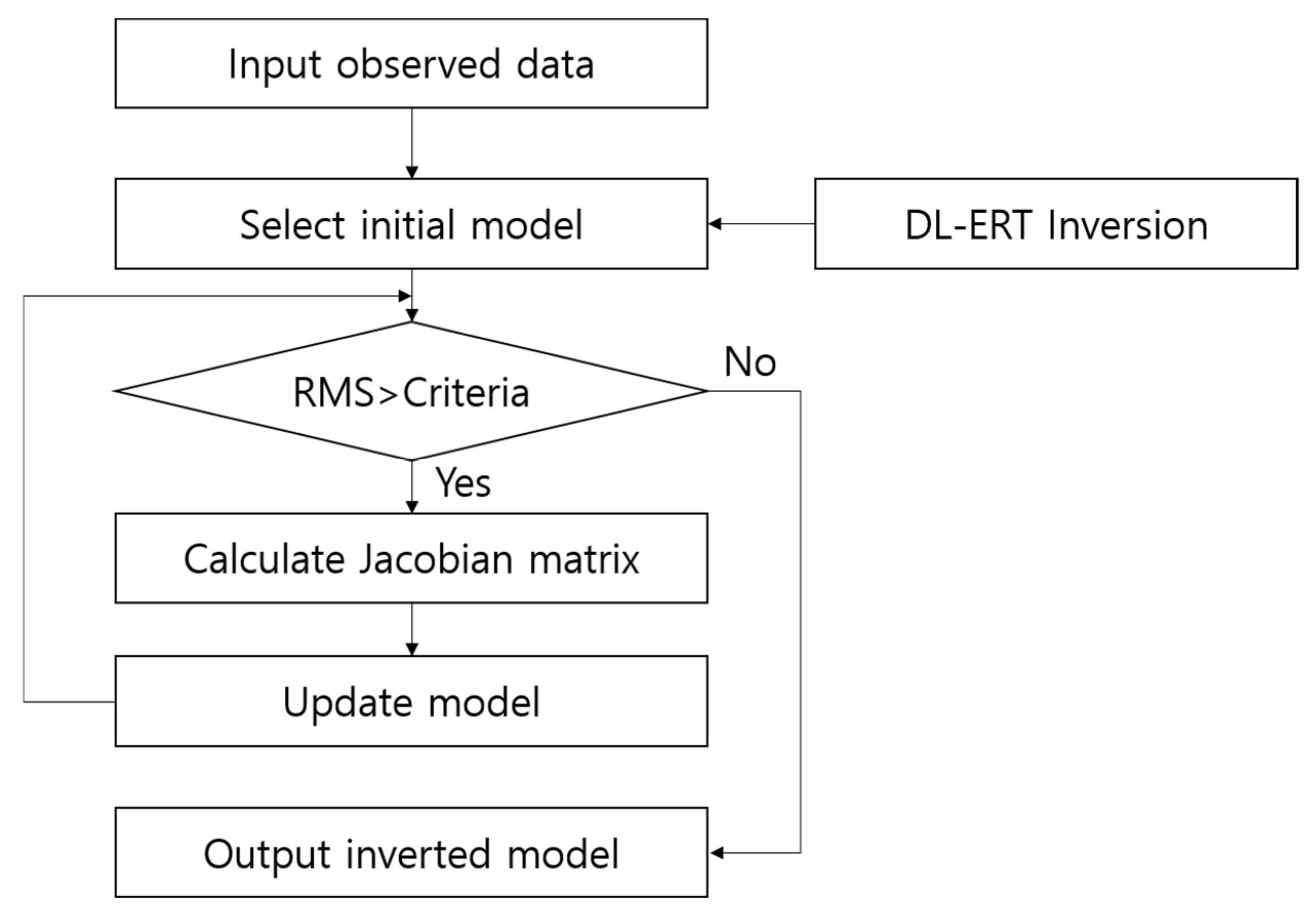
2.5. Deterministic Inversion Using Initial Model from DL-ERT Inversion

To improve our DL-ERT inversion, we leveraged field borehole data to generate more realistic and target-oriented training data. However, generating training data that accurately represents the complex subsurface structure and uncertainties found in real field data is challenging, which can limit the applicability of deep-learning models trained on synthetic data to actual field data.

Although deep-learning models aim to minimize the difference between the prediction and ground truth in the resistivity model, they may not fit the data as well as deterministic inversion methods, which are optimized to fit the data. However, deterministic inversion methods suffer from the ill-posed nature of the inverse problem, often leading to unstable results and convergence problems, particularly if the initial model is far from the actual subsurface properties. To address these issues, we implemented deterministic inversion using the results of DL-ERT inversion as the initial model. This approach provides a better solution with a more reliable starting point, improving the accuracy and reliability of our inversion results.

In this work, we used the SimPEG library for deterministic inversion, which solves the minimization problem with an objective function, $\Phi \left(\mathit{m}\right)$, that comprises a data misfit term, ${\Phi }_d\left(\mathit{m}\right),$ and a regularization term, ${\Phi }_m\left(\mathit{m}\right)$, as follows:

$$\Phi \left(\mathit{m}\right)={\Phi }_d\left(\mathit{m}\right)+\beta {\Phi }_m\left(\mathit{m}\right)=\Vert {\mathit{W}}_d{\left(F\left(\mathit{m}\right)-{\mathit{d}}_{obs}\right)\Vert }_2^2+\beta \Vert {\mathit{W}}_m{\left(\mathit{m}-{\mathit{m}}_{apr}\right)\Vert }_2^2,$$

(9)

where $\beta$ is the regularization parameter; ${\mathit{W}}_d$ and ${\mathit{W}}_m$ are data weights and model weights, respectively; $F$ is forward modeling; ${\mathit{d}}_{obs}$ denotes observed data. The prior information in the model is incorporated through the a priori model ${\mathit{m}}_{apr}$. Further details on the method can be found in [31].

Then, we used the Gauss–Newton method to solve the minimization of Equation (9). The flowchart of the deterministic inversion is presented in Figure 8. Typically, the initial model is assumed to be a homogeneous background model, which could be far from the true resistivity model and make it difficult to achieve convergence in the misfit. By contrast, we used the output of the DL-ERT inversion as the initial model and then ran the deterministic inversion. This approach allowed us to obtain better data fitting than the traditional deterministic inversion. In the next section, we demonstrate the effectiveness of our approach using synthetic test data and field data.

3. Experiment

3.1. Data Generation Using Borehole Information

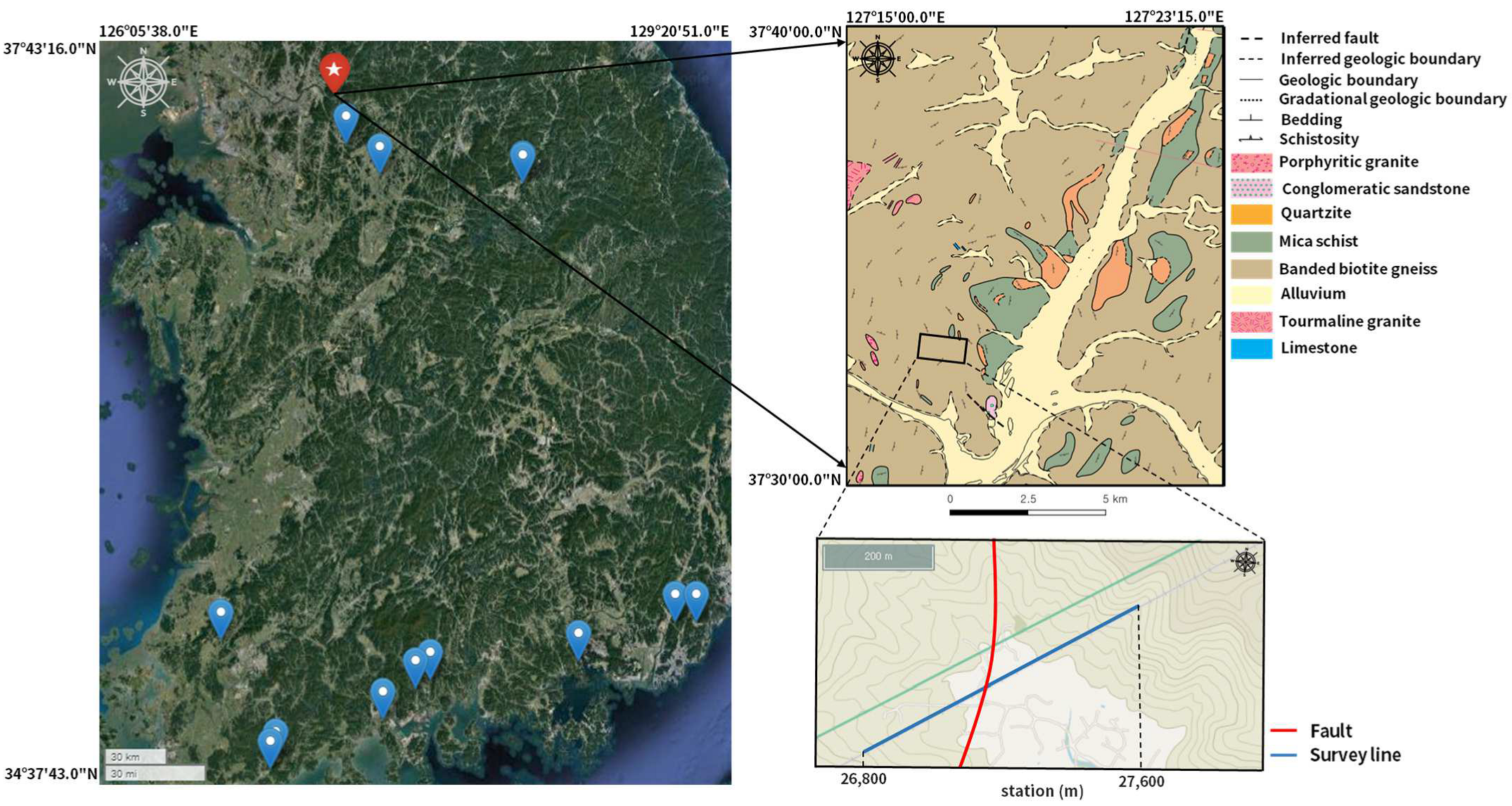
To generate target-oriented subsurface resistivity models, we used borehole data acquired from 13 drilling sites in South Korea, including Jangheung, Jangseong, Gwangyang, and Suncheon in South Jeolla Province; Changwon, Yangsan, and Hadong in South Gyeongsang Province; Gwangju and Icheon in Gyeonggi Province; Jecheon in North Chungcheong Province; and Gijang-gun in Busan. Figure 9 shows a map indicating the locations of the drilling sites. Each site is composed of various rock types, including gneiss, schist, phyllite, acidic dike, granite, andesite, granite, phyllite, tuff, limestone, and metamorphic sedimentary rocks originating from a wide range of geological eras from the Precambrian to the Mesozoic. Each site includes 5–19 borehole data, for a total of 150 borehole data used in this study. Each borehole data provides information on the Transverse Mercator (TM) coordinates, depth (m), Unified Soil Classification System (USCS), and stratum composition. On the basis of the electrical resistivity values of the strata, we categorized them into four layers: soil layer, weather ground layer, basement rock layer, and fault layer, as determined by USCS. The range of electrical resistivity values for each stratum was set as follows: 500–1000 ohm-m for the soil layer, 500–2000 ohm-m for the weather ground layer, 1000–3000 ohm-m for the basement rock layer, and 200–500 ohm-m for the faults [36,37]. It is important to note that there may be some overlap in the resistivity values between different strata. This is primarily due to the presence of mixed rock types within the field borehole data, which cannot be easily categorized into a single specific stratum. Then, the borehole information, including the coordinates, depth, and resistivity values, was used to generate resistivity models, with resistivity values randomly selected from within the specified range.

Employing the borehole information described above, we generated 3D resistivity models using GemPy. The 3D model was set to 200 × 10 × 200 m in the x, y, and z directions, respectively, and composed of three layers, namely, the soil layer, weathered ground layer, and basement layer, according to the field borehole data. We then added the fault layer to the layered model with a randomly selected dip angle ranging from 45° to 90° and thickness ranging from 20 to 100 m.

For the forward modeling using SimPEG, we set the survey as a dipole–dipole array with a range of −320–320 m. The spacing between the electrodes was set to 20 m, and the maximum number of repetitions of the receiver for each transmitter was limited to 10.

In this way, we generated 5000 sets of synthetic data, including layered models with and without a fault structure, and split them into training, validation, and test data sets with a 7:2:1 ratio. It is important to note that only one fault layer was added for the fault model at this stage; however, we also set additional test data with two fault layers to evaluate the generalization capability of the inversion model.

3.2. Data Preprocessing

The MinMax scaler was used for the apparent resistivity data and resistivity models, which were inputs and labels of the deep-learning model. In the case of the apparent resistivity data, NaN values outside the inverted trapezoid were converted to zero after scaling. The inputs and labels were resized to 64 × 128. To avoid overfitting and improve generalization performance, data augmentation was performed by applying horizontal flipping to the training data only.

3.3. Training DL Inversion Networks

The training of the model was divided into three stages: base model training, borehole mixer training, and fine tuning. We used the Adam optimizer with a batch size of 256 and a maximum of 300 epochs. The learning rates were set to be different in each stage, decreasing by a factor of 10 each time, from 10⁻³ to 10^-−5 in the three stages. Figure 10 shows the loss curve for base model training, borehole mixer training, and fine tuning. All experiments were carried out on TensorFlow 2, and two GPUs (NVIDIA GeForce RTX 2090 Ti) were used to accelerate computation.

3.4. Evaluating the Performance of DL Inversion Models Using Synthetic Test Dataset

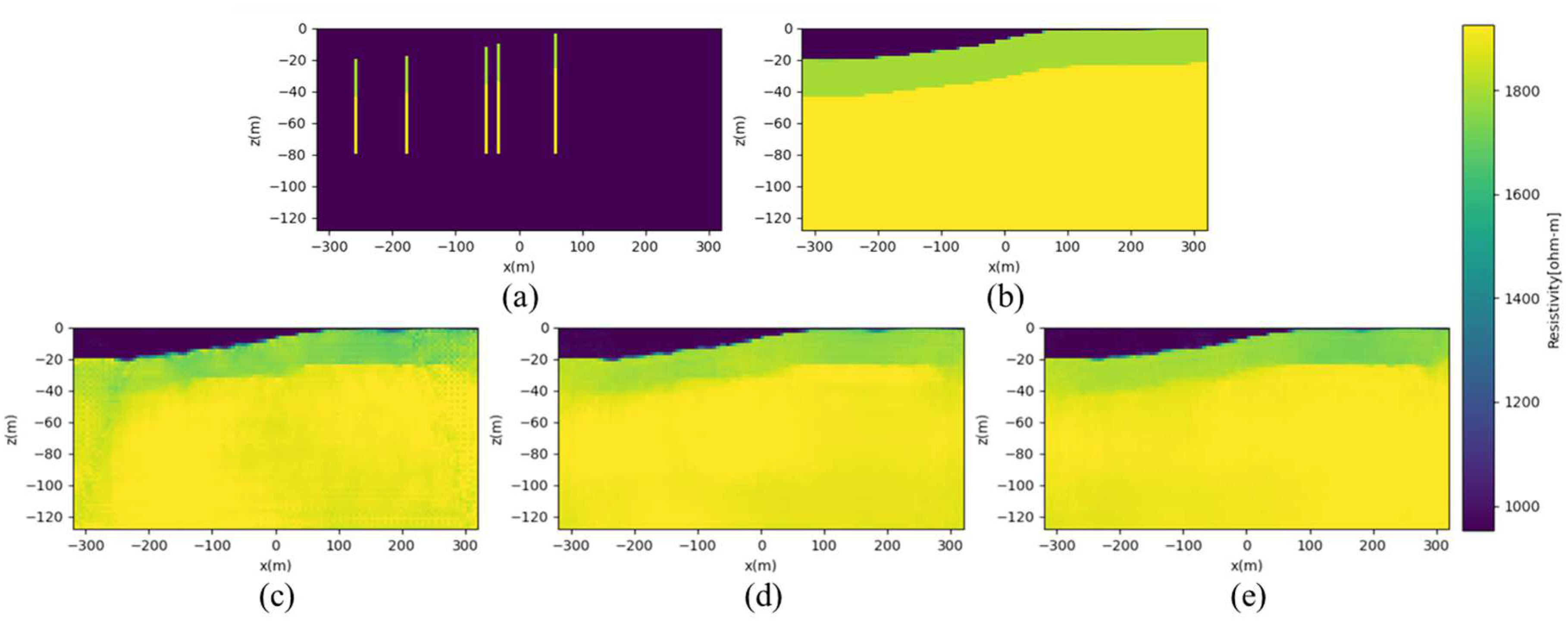
After training the models in the three stages, the performance of each model was evaluated by comparing the results on the test datasets, which consisted of the layered, one-fault, and two-fault structures. The normalized root-mean-squared error (NRMSE), which is calculated by normalizing the root-mean-squared error (RMSE) by the difference between the maximum and minimum values, was used to quantify the performance of the trained inversion models. In Figure 11, the base model without a borehole mixer and borehole information shows promising results; however, the fine-tuning model shows the clearest and most similar results to the ground truth with the lowest NRMSE. 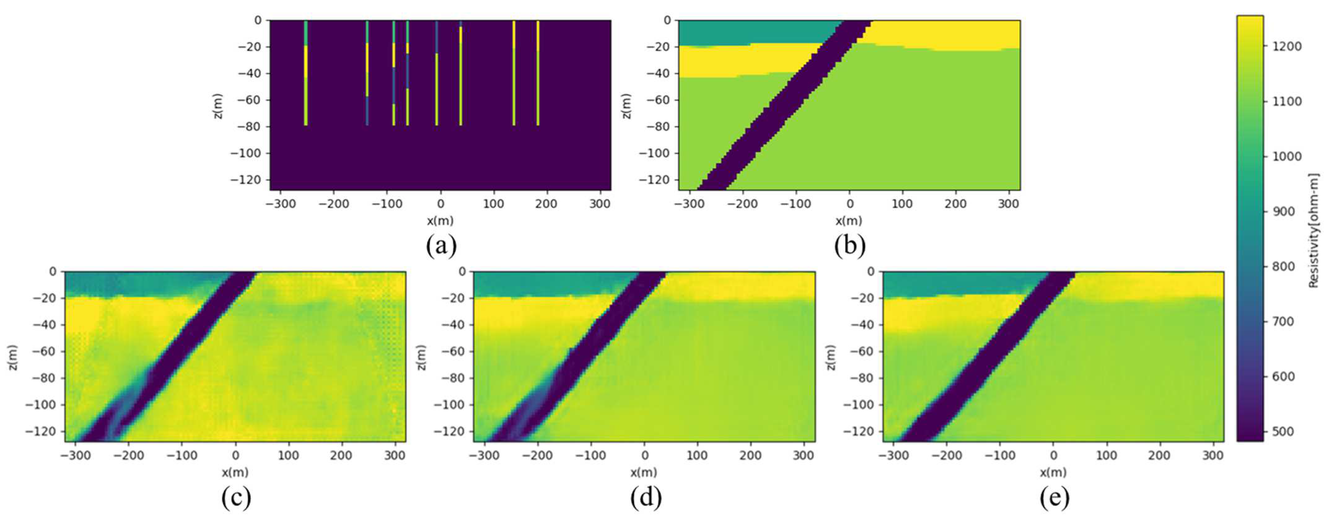Similarly, as shown in Figure 12, for a one-fault structure, all three models predicted the fault zone very clearly, but artifact noise is observed in the base model. The artifacts disappeared in borehole mixer training and fine-tuning, confirming results that incorporating the borehole information in the borehole mixer network helps predict the weather ground layer, which the base model cannot predict. 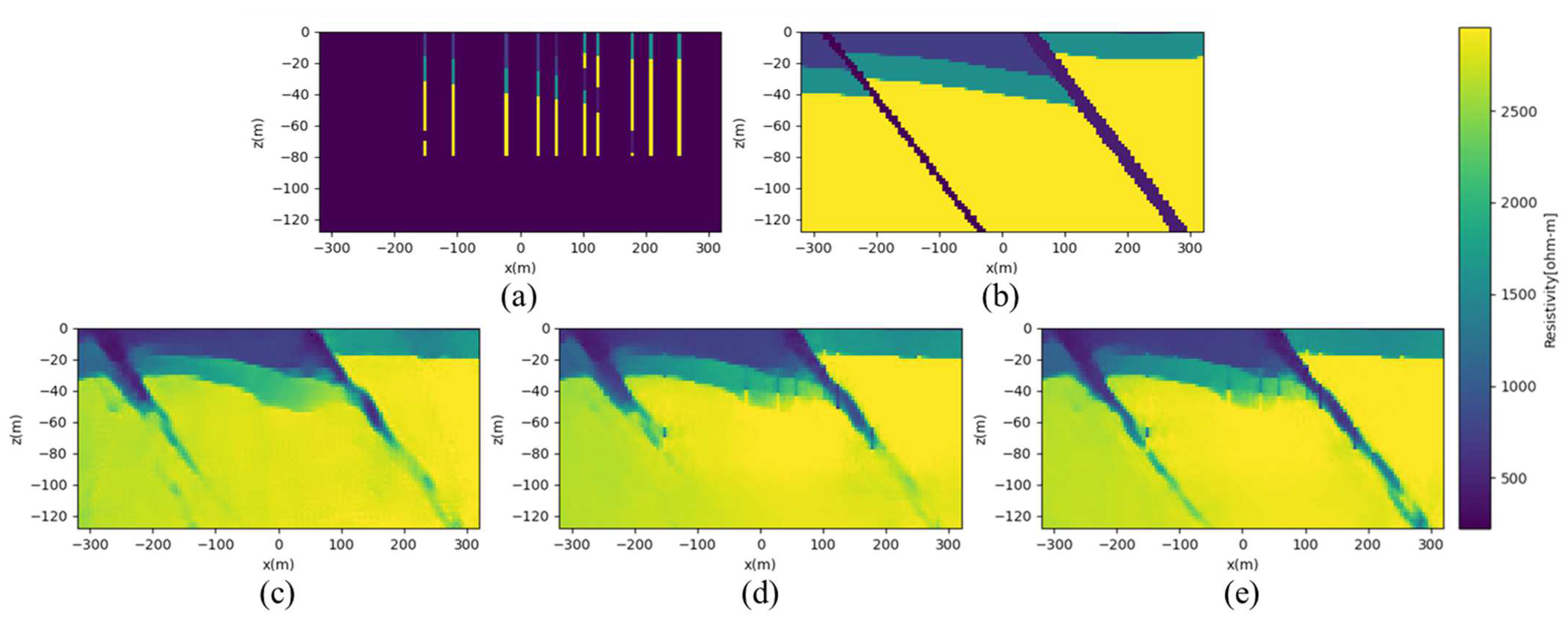To verify the generalization performance of the deep-learning model, prediction results were also compared for the two-fault structure, and the fine-tuning model exhibited the best performance, as shown in Figure 13. It is important to note that a two-fault structure was not included in the training dataset, which only consisted of a one-fault model. By evaluating the model’s performance on an unseen fault configuration, we were able to gauge its ability to generalize beyond the specific training data. Moreover, a comparsion of the prediction results of the three types of test datarevealed that the fine-tuning model provided the highest prediction accuracy.

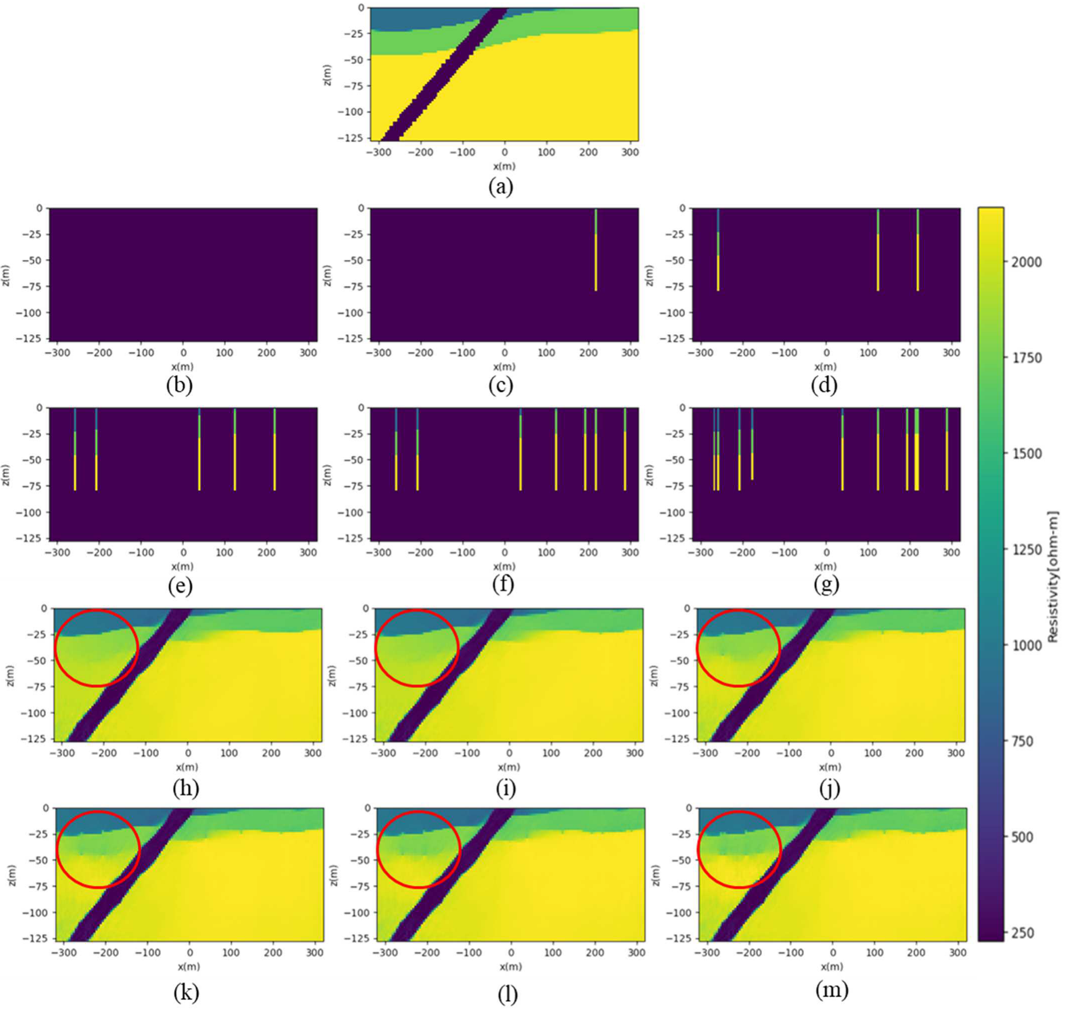
Additionally, to evaluate the effectiveness of the mixer network incorporating borehole information, we compared the results of the fine-tuning model with data from an increasing number of borehole data. As shown in Figure 14, as the number of boreholes increases, the NRMSE value gradually decreases with less artifact noise and clearer layered structures. Notably, when examining the red circles in Figure 14i–m, it is evident that an increase in the number of boreholes from zero to one, one to two, and two to four progressively enhanced the distinction of the three layers. Additionally, when there was no change in the borehole configuration within the red circles, the NRMSE showed a slight decrease. However, with changes in the borehole configuration, the NRMSE exhibited a significant decrease. These findings emphasize that both the number and distribution of boreholes play a crucial role in the inversion’s performance.

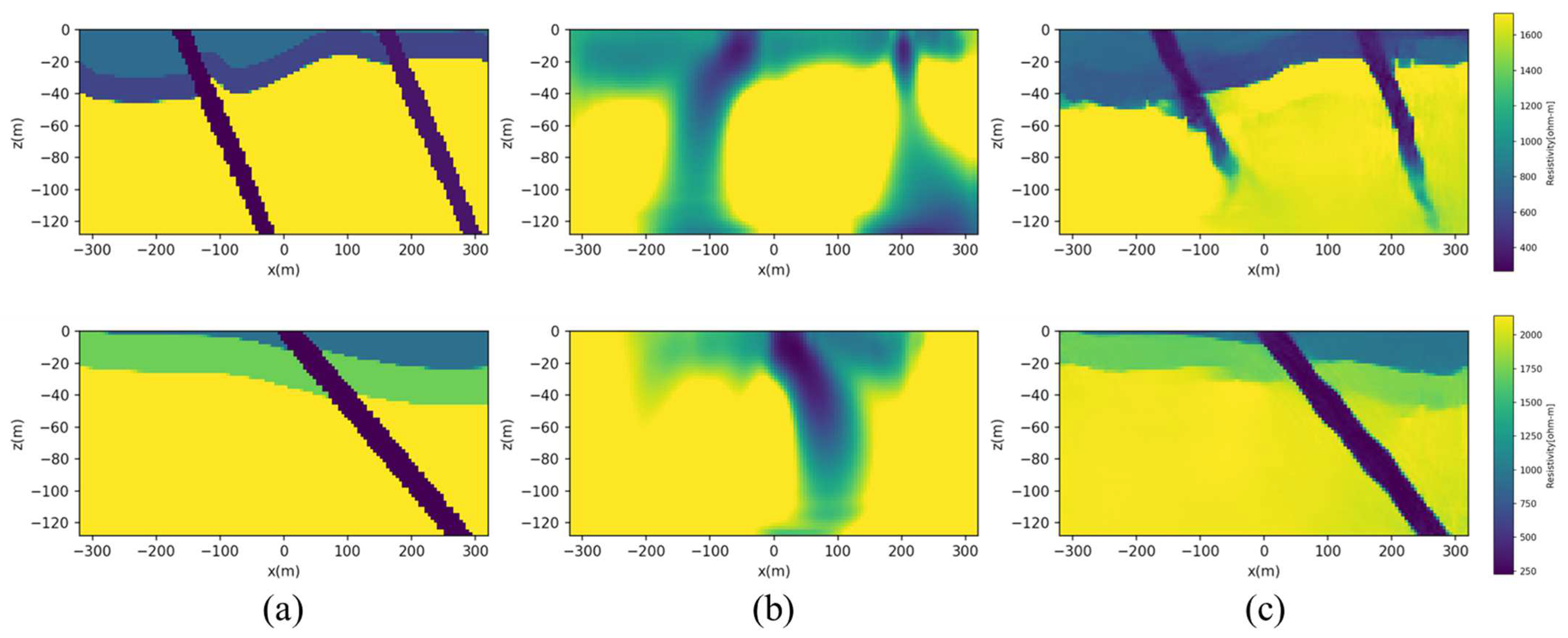
Finally, we compared our results with those from conventional deterministic inversion methods. In this work, we used the conventional smoothing least-squares inversion method with SimPEG. As shown in Figure 15, the deep learning-based model shows superior prediction accuracy compared with the conventional inversion method, as it more accurately predicts the layers and the direction and position of the fault zone.

3.5. Field Data Application

To demonstrate the efficacy and accuracy of the proposed approaches, we utilized field data from a railway tunnel construction site in Namyangju and Yangpyeong, Gyeonggi Province, South Korea. This area belongs to the central part of the Gyeonggi Massif, which is generally referred to as the basement rock of the Korean Peninsula, and the third-grade deep fault called the Gyeonggang Fault, which is known as a large-scale tectonic formation, passes through this area [36]. This area is mainly composed of Cambrian strata of the banded biotite gneiss, and small-scale rock bodies of mica schist and quartzite are isolated as structural enclaves [38]. The surveyed area has developed faults parallel to the foliation and is characterized by a fault zone with a width of approximately 10 m, identified through surface geological surveys. The geologic plan map of the surveyed area is shown in Figure 9. The electrical resistivity equipment used is the SuperSting R8/IP by AGI (Austin, TX, USA), with a maximum voltage of 800 Vp-p and a maximum current of 2.0 A. During field surveys, the contact resistance typically ranges from 1 to 2 kΩ, and the output current is around 200 to 300 mA. We conducted DC resistivity surveys using a dipole–dipole electrode configuration with a survey line length of 400 m, a dipole spacing of 20 m, and a maximum number of iterations per transmitter of 8. Unfortunately, borehole data were not available in the survey area, therefore, we performed DL-ERT inversion without incorporating borehole data.

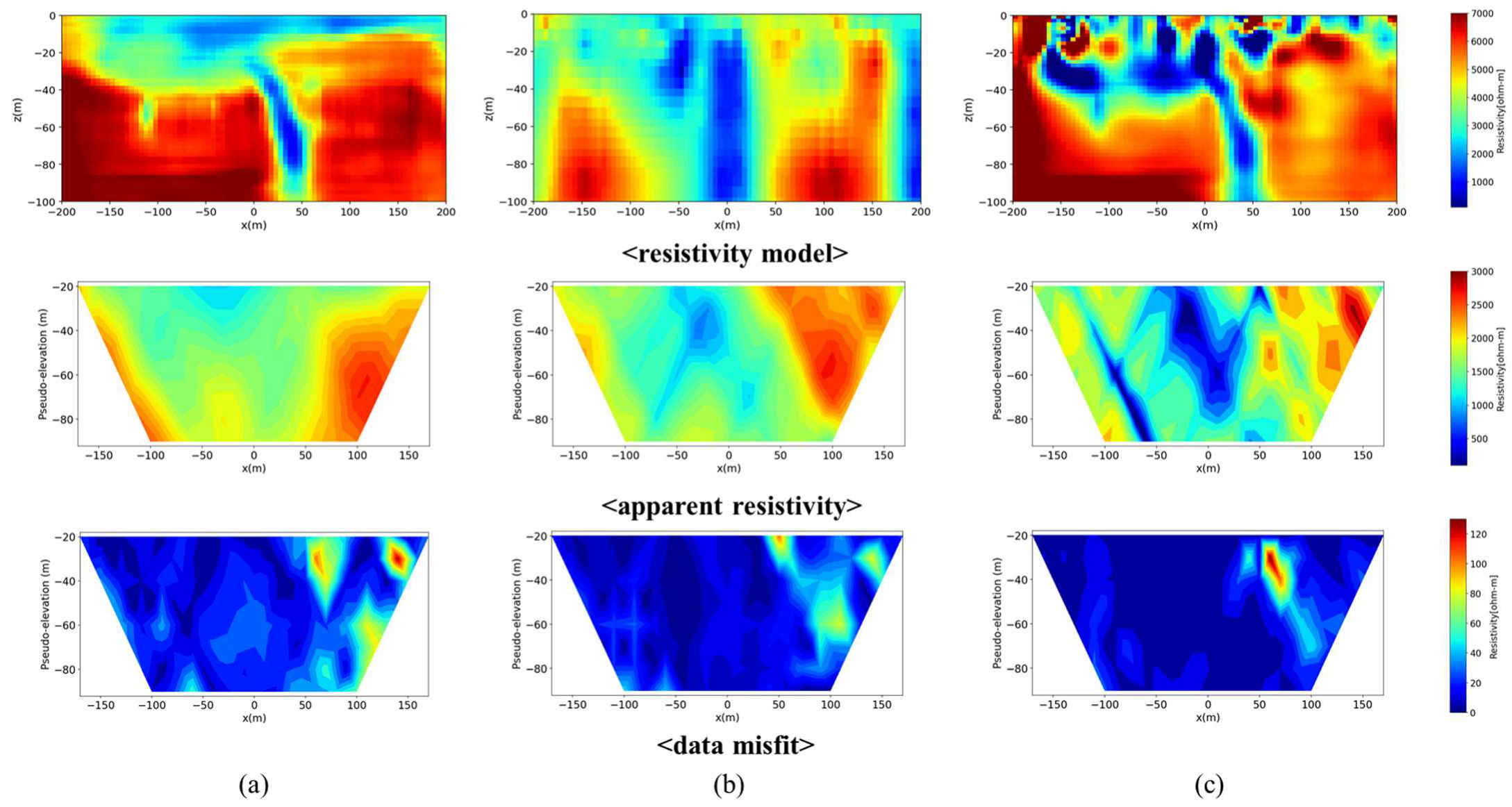
We compared the results of three methods, namely, DL-ERT inversion, deterministic inversion, and deterministic inversion with a DL-ERT initial model. Figure 15 presents the recovered models, the computed apparent resistivity data from the recovered models, and the differences between calculated and observed data for the three different approaches. All three models exhibited similar outcomes, with a conductive fault zone located at the center and resistive basement rock located on the sides of the survey area. However, the deterministic inversion approach displayed a steeper dip angle of the fault and less sharp boundaries of the fault and basement structures compared with the other methods. Because no ground truth or borehole data were available for validation, we computed the apparent resistivity data using electrical resistivity forward modeling and determined the RMSE (${\mathrm{RMSE}}_d$) between the measured data from the recovered model and the observed data. The ${\mathrm{RMSE}}_d$ value was obtained from the data misfit defined in Equation (9) as follows:

$${\mathrm{RMSE}}_d=\sqrt{{\mathsf{\Phi }}_d/N },$$

(10)

where N is the number of data points.

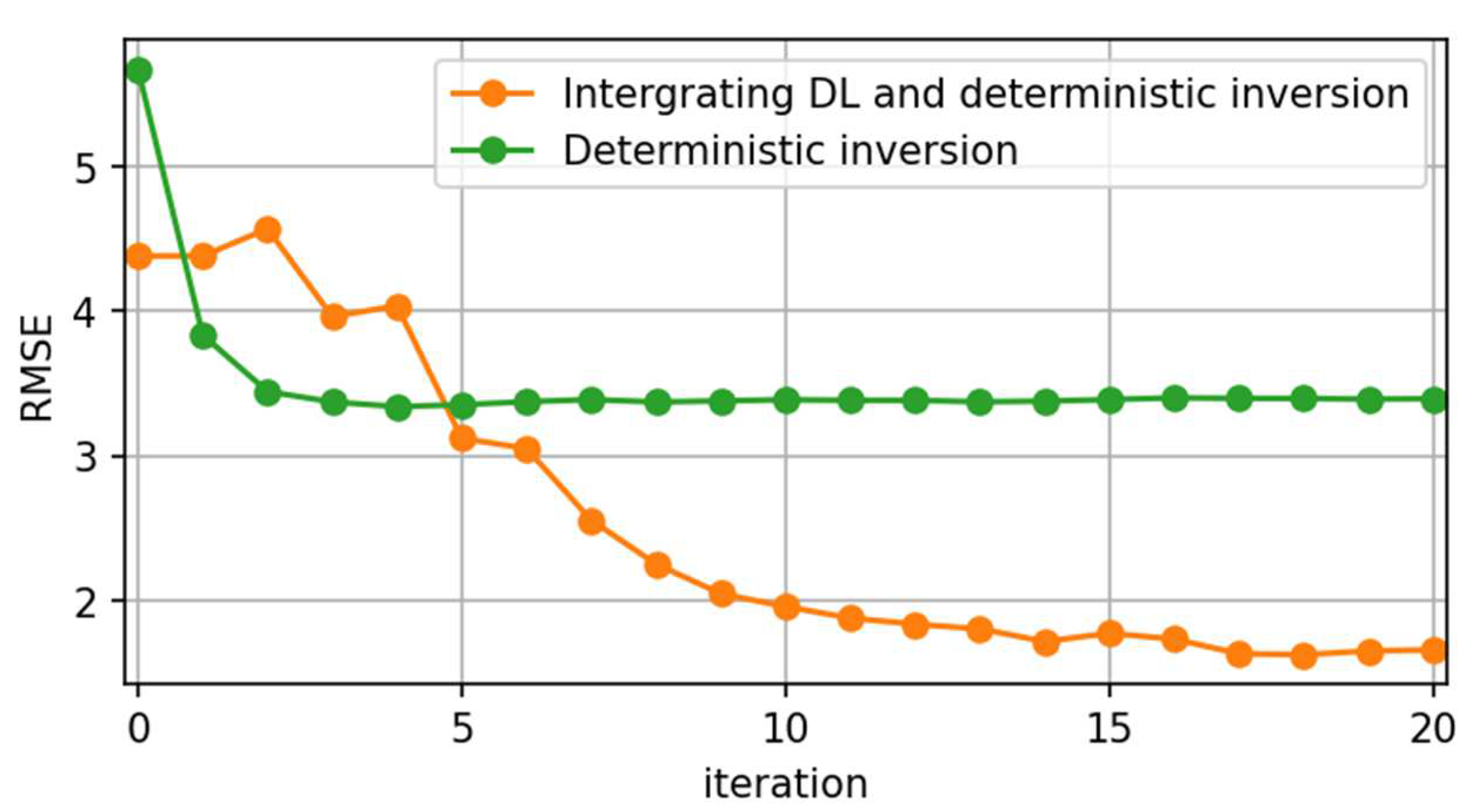
The ${\mathrm{RMSE}}_d$ of the DL-ERT inversion was calculated as 4.3832, while the deterministic inversion after 20 iterations was 3.3959, as shown in Figure 16. The deterministic inversion exhibits a better fit to the data in terms of data misfit, indicating a limitation in the applicability of deep-learning models when synthetic training data differ from the target field data. However, it is worth noting that the data misfit of the traditional deterministic inversion shown in Figure 17 does not decrease significantly beyond four iterations, indicating that it may become trapped in a local minimum. However, when the recovered model from the DL-ERT inversion was used as the initial model for the deterministic inversion, the ${\mathrm{RMSE}}_d$ value decreased continuously and reached 1.6595 after 20 iterations. This significant improvement demonstrates the effectiveness of using the DL-ERT inversion as a starting point to enhance the accuracy and data fitting in the deterministic process.

Therefore, the proposed approach, which integrates deterministic inversion with the DL-ERT initial model, can provide a better solution than DL-ERT or deterministic inversion alone, leading to improved accuracy and data fitting. This finding suggests that the combination of deep learning and deterministic inversion methods could be a promising approach for solving inversion problems.

4. Discussion

In this study, we propose a methodology that utilizes field borehole data to create target-oriented resistivity models. However, it is important to acknowledge that the resistivity models generated in this study are relatively simple, typically comprising of two or three layers with linear faults. This simplicity arises from the nature of the acquired field borehole data, which exhibit a relatively simple lithology characterized by a few distinct layers. Nonetheless, we believe that our proposed workflow can be extended to create more complex resistivity models by incorporating field borehole data from lithologically diverse and complex regions.

Despite the promising results obtained from our methodology, several limitations warrant further attention. Firstly, our current deep-learning model is designed for 2D resistivity models and 2D survey data, lacking the inclusion of 3D effects that are crucial for accurately inverting field data. Incorporating three-dimensional considerations into our model will enhance its ability to capture the true complexity of subsurface resistivity distributions.

Secondly, topographical information plays a vital role in the modeling and inversion processes. However, our current deep-learning model does not account for topographical effects. Future improvements to our methodology should focus on integrating topographical data to enhance the accuracy and reliability of the inversion results.

Thirdly, when generating resistivity models with faults, we only considered a single-fault structure with a linear shape. Although this approach provides valuable insights, it may not fully capture the diverse range of fault structures encountered in real-world scenarios. Expanding the fault modeling capability of our methodology to incorporate various fault geometries will be an important area of future investigation.

Additionally, it is worth noting that the training data used in this study were generated without considering noise. Including noise in the training data would enable the deep-learning model to better handle real-world data characterized by various noise sources and levels.

Furthermore, for the training data, we intentionally used a wide electrode spacing of 20 m. This choice was made because a smaller electrode spacing would require more data points in the apparent resistivity map to cover the same survey area, resulting in a larger input and output size for the deep-learning model and increased computational memory requirements. The electrode spacing plays a crucial role in the sensitivity of detecting faults. In our study, we considered a fault thickness ranging from 20 to 100 m, taking into account the electrode spacing of 20 m. Therefore, to detect thin faults, a shorter electrode spacing and larger input and output data sizes for DL-ERT inversion need to be considered.

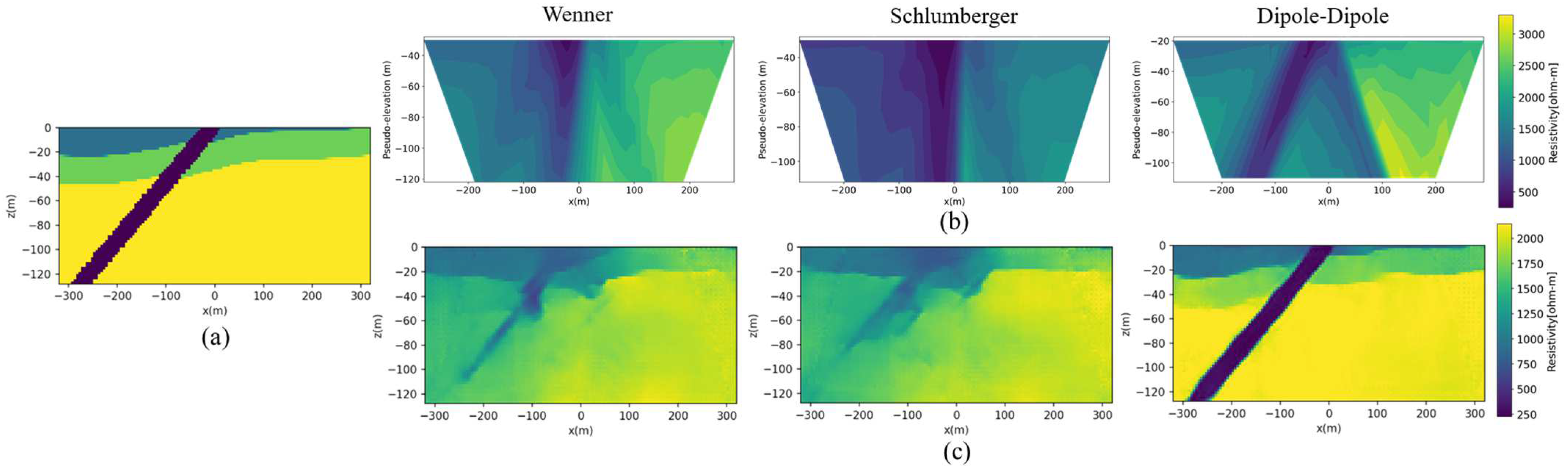
Lastly, our current DL-ERT inversion model has been specifically trained for the dipole–dipole array configuration. Consequently, applying the model to other electrode configurations may yield suboptimal results due to inherent differences in data characteristics. We conducted an experiment comparing the performance of our model with Wenner, Schlumberger, and dipole–dipole arrays (Figure 18), confirming that our current DL-ERT model is not well-suited for non-dipole–dipole arrays. Addressing this limitation and developing a more versatile model capable of accommodating different electrode configurations will be the focal point of our future research.

In our field data example, even though the comparison of the convergence curves between deterministic inversion with and without the DL-ERT initial model implies the effectiveness of our proposed workflow, it is worth mentioning that to fully demonstrate the efficacy of our approach, it would be beneficial to have borehole data for a direct comparison of the results.

In summary, while our proposed methodology has demonstrated promising results, it is important to acknowledge and address the limitations outlined above. Future research efforts will focus on extending our model to incorporate 3D effects, integrating topographical information, enhancing fault modeling capabilities, considering noise in the training data, and developing a more versatile approach capable of handling different electrode configurations. By addressing these limitations, we aim to advance the field of DL-ERT inversion and improve its applicability to real-world scenarios.

5. Conclusions

In this paper, we present a novel approach for integrating deep learning and deterministic inversion for electrical resistivity surveys. The proposed workflow involves generating a target-oriented training dataset based on field borehole data and training the deep-learning model in three stages: base model training, borehole mixer training, and fine-tuning. The base model performs pure resistivity inversion without borehole information, while the mixer network incorporates borehole data into the inversion result. In the fine-tuning stage, we slightly adjust the model parameters for better performance. In addition, to overcome the limitation of deep-learning models when synthetic training data differs from target field data, we use the recovered model from DL-ERT inversion as an initial model for the deterministic inversion. We tested our approach using both synthetic test data and field data from a railway tunnel construction site in South Korea, and our proposed method, which combines deterministic inversion with a DL-ERT initial model, was designed to outperform DL-ERT or deterministic inversion alone in terms of accuracy and data fitting. Our findings suggest that the combination of deep learning and deterministic inversion methods holds great promise for solving inversion problems. The proposed approach can potentially be extended to other geophysical methods and geological scenarios to improve the accuracy and efficiency of inversion solutions.

References

- Shin, H.; Choon, S. Civil Structure Construction and Fault. J. Korean Tunn. Undergr. Space Assoc. 1999, 1, 39–49. [Google Scholar]
- Cho, K.; Kim, K.S.; Lee, K.S. 3D resistivity survey at a collapsed tunnel site. Geophys. Geophys. Explor. 2015, 18, 14–20. [Google Scholar] [CrossRef]
- Moon, S.W.; Yun, H.S.; Choo, C.O.; Kim, W.S.; Seo, Y.S. A Study on Mineralogical and Basic Mechanical Properties of Fault Gouges in 16 Faults. J. Miner. Soc. Korea 2015, 28, 109–126. [Google Scholar] [CrossRef]
- Wei, X.L.; Zhang, C.X.; Kim, S.W.; Jing, K.L.; Wang, Y.J.; Xu, S.; Xie, Z.Z. Seismic fault detection using convolutional neural networks with focal loss. Comput. Geosci. 2021, 158, 104968. [Google Scholar] [CrossRef]
- Pochet, A.; Diniz, P.H.; Lopes, H.; Gattass, M. Seismic fault detection using convolutional neural networks trained on synthetic poststacked amplitude maps. IEEE Geosci. Remote Sens. Lett. 2018, 16, 352–356. [Google Scholar] [CrossRef]
- Barnes, H.; Hinojosa, J.R.; Spinelli, G.A.; Mozley, P.S.; Koning, D.; Sproule, T.G.; Wilson, J.L. Detecting fault zone characteristics and paleovalley incision using electrical resistivity: Loma Blanca Fault, New Mixoco. Geophysics 2021, 86, B209–B221. [Google Scholar] [CrossRef]
- Torrese, P.; Pilla, G.; Bersan, M.; Rainone, M.L.; Ciancetti, G. Mapping the uprising of highly mineralized waters occurring along a fault zone in the Oltrepò Pavese plain upper aquifers (Northern Italy) using VLF-EM survey. In Proceedings of the SAGEEP 22nd Annual Meeting, Fort Worth, TX, USA, 25 June 2009. [Google Scholar]
- Nurhasan; Ogawa, Y.; Kimata, F.; Sutarno, D.; Sugiyanto, D.; Ismail, N. Identification of Sumatran fault zone using magnetotelluric and gravity data. In Proceedings of the 13th SEGJ International Symposium, Tokyo, Japan, 29 April 2019. [Google Scholar]
- Saribudak, M.; Ruder, M.; Van Nieuwenhuise, B. Hockley Fault revisited: More geophysical data and new evidence on the fault location, Houston, Texas. Geophysics 2018, 83, B133–B142. [Google Scholar] [CrossRef]
- Park, M.K. Laboratory study on the electrical resistivity characteristics with contents of clay minerals. Geophys. Geophys. Explor. 2005, 8, 218–223. [Google Scholar]
- Rønning, J.S.; Ganerød, G.V.; Dalsegg, E.; Reiser, F. Resistivity mapping as a tool for identification and characterisation of weakness zones in crystalline bedrock: Definition and testing of an interpretational model. Bull. Eng. Geol. Environ. B Eng. Geol. Environ. 2014, 73, 1225–1244. [Google Scholar] [CrossRef]
- Ganerød, G.V.; Rønning, J.S.; Dalsegg, E.; Elvebakk, H.; Holmøy, K.; Nilsen, B.; Braathen, A. Comparison of geophysical methods for sub-surface mapping of faults and fracture zones in a section of the Viggja road tunnel, Norway. Bull. Eng. Geol. Environ. B Eng. Geol. Environ. 2006, 65, 231–243. [Google Scholar] [CrossRef]
- Zhu, T.; Zhou, J.; Wang, H. Localization and characterization of the Zhangdian-Renhe fault zone in Zibo city, Shandong province, China, using electrical resistivity tomography (ERT). Appl. Geophys. 2017, 136, 343–352. [Google Scholar] [CrossRef]
- Tassis, G.; Rønning, J.S.; Tsourlos, P.; Dahlin, T. Marine ert modeling for the detection of fracture zones. In Proceedings of the SAGEEP 2015, Austin, TX, USA, 22–26 March 2015. [Google Scholar]
- Zhu, T.; Feng, R.; Hao, J.Q.; Zhou, J.G.; Wang, H.L.; Wang, S.Q. The application of electrical resistivity tomography to detecting a buried fault: A case study. J. Environ. Eng. Geophys. 2009, 14, 145–151. [Google Scholar] [CrossRef]
- Ioane, D.; Chitea, F.; Diacopolos, C.; Stochici, R. Active faults detected in urban areas using ves and ert geophysical techniques study case: Bucharest, Romania. In Proceedings of the Geoscience 2016, Bucharest, Romania, 25 November 2016. [Google Scholar]
- Sana, H.; Taborik, P.; Valenta, J.; Bhat, F.A.; Flašar, J.; Štěpančíkova, P.; Khwaja, N.A. Detecting active faults in intramountain basins using electrical resistivity tomography: A focus on Kashmir Basin, NW Himalaya. Appl. Geophys. 2021, 192, 104395. [Google Scholar] [CrossRef]
- Araya-Polo, M.; Dahlke, T.; Frogner, C.; Zhang, C.; Poggio, T.; Hohl, D. Automated fault detection without seismic processing. Lead. Edge 2017, 36, 208–214. [Google Scholar] [CrossRef]
- Jeong, J.; Jang, H.; Caesary, D.; Joung, I.S.; Cho, A.; Yoon, D.; Nam, M.J. Research Trends and Case Studies of Deep Learning Applications in Geo-electric and Electromagnetic Surveys. J. Korean Soc. Miner. Energy Resour. Eng. 2022, 59, 379–397. [Google Scholar] [CrossRef]
- Liu, B.; Guo, Q.; Li, S.; Liu, B.; Ren, Y.; Pang, Y.; Guo, X.; Liu, L.; Jiang, P. Deep learning inversion of electrical resistivity data. IEEE Trans. Geosci. Remote. Sens. 2020, 58, 5715–5728. [Google Scholar] [CrossRef]
- Liu, B.; Guo, Q.; Wang, K.; Pang, Y.; Nie, L.; Jiang, P. Adaptive Convolution Neural Networks for Electrical Resistivity Inversion. IEEE Sens. J. 2020, 21, 2055–2066. [Google Scholar] [CrossRef]
- Vu, M.T.; Jardani, A. Convolutional neural networks with SegNet architecture applied to three-dimensional tomography of subsurface electrical resistivity: CNN-3D-ERT. Geophys. J. Int. 2021, 225, 1319–1331. [Google Scholar] [CrossRef]
- Wilson, B.; Singh, A.; Sethi, A. Appraisal of resistivity inversion models with convolutional variational encoder-decoder network. IEEE Trans. Geosci. Remote Sens. 2022, 60, 1–10. [Google Scholar] [CrossRef]
- Oh, S.; Noh, K.; Yoon, D.; Seol, S.J.; Byun, J. Salt delineation from electromagnetic data using convolutional neural networks. IEEE Geosci. Remote Sens. Lett. 2018, 16, 519–523. [Google Scholar] [CrossRef]
- Noh, K.; Yoon, D.; Byun, J. Imaging subsurface resistivity structure from airborne electromagnetic induction data using deep neural network. Explor. Geophys. 2020, 51, 214–220. [Google Scholar] [CrossRef]
- Li, J.; Liu, Y.; Yin, C.; Ren, X.; Su, Y. Fast imaging of time-domain airborne EM data using deep learning technology. Geophysics 2020, 85, E163–E170. [Google Scholar] [CrossRef]
- Wu, X.; Xue, G.; Zhao, Y.; Lv, P.; Zhou, Z.; Shi, J. A deep learning estimation of the earth resistivity model for the airborne transient electromagnetic observation. J. Geophys. Res. 2022, 127, e2021JB023185. [Google Scholar] [CrossRef]
- de la Varga, M.; Schaaf, A.; Wellmann, F. GemPy 1.0: Open-source stochastic geological modeling and inversion. Geosci. Model Dev. 2019, 12, 1–32. [Google Scholar] [CrossRef]
- Lajaunie, C.; Courrioux, G.; Manuel, L. Foliation fields and 3D cartography in geology: Principles of a method based on potential interpolation. Math. Geol. 1997, 29, 571–584. [Google Scholar] [CrossRef]
- Calcagno, P.; Chilès, J.P.; Courrioux, G.; Guillen, A. Geological modelling from field data and geological knowledge: Part I. Modelling method coupling 3D potential-field interpolation and geological rules. Phys. Earth Planet. Inter. 2008, 171, 147–157. [Google Scholar] [CrossRef]
- Cockett, R.; Kang, S.; Heagy, L.J.; Pidlisecky, A.; Oldenburg, D.W. SimPEG: An open source framework for simulation and gradient based parameter estimation in geophysical applications. Comput. Geosci. 2015, 85, 142–154. [Google Scholar] [CrossRef]
- Ronneberger, O.; Fischer, P.; Brox, T. U-net: Convolutional networks for biomedical image segmentation. In Proceedings of the MICCAI, Munich, Germany, 5–9 October 2015. [Google Scholar]
- Ioffe, S.; Szegedy, C. Batch normalization: Accelerating deep network training by reducing internal covariate shift. In Proceedings of the ICML, Lille, France, 6–11 July 2015. [Google Scholar]
- Agarap, A.F. Deep learning using rectified linear units (ReLU). arXiv 2018, arXiv:1803.08375. [Google Scholar]
- Nava, L.; Cuevas, M.; Meena, S.R.; Catani, F.; Monserrat, O. Artisanal and small-scale mine detection in semi-desertic areas by improved U-Net. IEEE Geosci. Remote Sens. Lett. 2022, 19, 1–5. [Google Scholar] [CrossRef]
- Kwon, H.S.; Hwang, S.H.; Baek, H.J.; Kim, K.S. A study on the correlation between electrical resistivity and rock classification. Geophys. Geophys. Explor. 2008, 11, 350–360. [Google Scholar]
- Loke, M.H. Tutorial: 2-D and 3-D Electrical Imaging Survey; University of Alberta: Edmonton, AB, Canada, 2004; Available online: https://sites.ualberta.ca/~unsworth/UA-classes/223/loke_course_notes.pdf (accessed on 12 May 2023).
- Hong, S.H.; Oh, I.; Kim, H.; Lee, B.J. Numerical Geometry_50,000 Scale_Yangsu-ri. Available online: https://data.kigam.re.kr/data/7503d484-5613-429c-b741-fc2ded9fc360 (accessed on 2 May 2023).
Figure 1.
Proposed workflow for deep learning-based ERT inversion (DL-ERT) and integration with deterministic inversion.
Figure 2.
Geological structures created using GemPy: (a) layered structure, (b) fault structure, and (c) saturated fault structure.
Figure 3.
Three-dimensional lithological model generated using field borehole data.
Figure 4.
Two-dimensional lithological model and resistivity model generated in (a) GemPy and (b) SimPEG, respectively.
Figure 5.
(a) Pseudosection’s setting and observation points in pseudo-elevation for dipole–dipole array, and (b) corresponding pseudosection of apparent resistivity data.
Figure 6.
DL-ERT inversion network comprising a base model and a borehole mixer.
Figure 7.
Input of the mixer network incorporating the borehole feature map.
Figure 8.
Flowchart of the deterministic inversion with the initial model from the DL-ERT inversion.
Figure 9.
A map indicating the locations of the drilling area and electrical resistivity survey area in South Korea.
Figure 10.
Loss curves for base model training, borehole mixer training, and fine-tuning of the DL-ERT inversion.
Figure 11.
Prediction results of DL-ERT inversion for the layered structure: (a) boreholes injected during training, (b) ground truth, (c) base model result: NRMSE = 0.0355, (d) borehole mixer training result: NRMSE = 0.0245, and (e) fine-tuning result: NRMSE = 0.0235.
Figure 12.
Prediction results of DL-ERT inversion for the one-fault structure: (a) boreholes injected during training, (b) ground truth, (c) base model result: NRMSE = 0.0343, (d) borehole mixer training result: NRMSE = 0.0272, and (e) fine-tuning result: NRMSE = 0.0217.
Figure 13.
Prediction results of DL-ERT inversion for the two-fault structure: (a) boreholes injected during training, (b) ground truth, (c) base model result: NRMSE = 0.0115, (d) borehole mixer training result: NRMSE = 0.0076, (e) fine-tuning result: NRMSE = 0.0049.
Figure 14.
Prediction results of DL-ERT inversion according to the number of boreholes. The NRMSE values obtained with an increase in the number of boreholes are 0.0707, 0.0706, 0.0689, 0.0680, 0.0679, and 0.0669. (a) Ground truth. Number of boreholes = (b,h) 0; (c,i) 1; (d,j) 3; (e,k) 5; (f,l) 7; and (g,m) 10.
Figure 15.
Comparison of deterministic inversion and DL-ERT inversion: (a) ground truth, (b) deterministic inversion results, and (c) DL-ERT inversion results.
Figure 16.
Recovered models (top), corresponding apparent resistivities (middle), and differences between calculated and observed data (bottom) for (a) DL-ERT inversion, (b) deterministic inversion, and (c) deterministic inversion using the initial model from DL-ERT inversion.
Figure 17.
Convergence curves of deterministic inversion and integrating DL-ERT with deterministic inversion.
Figure 18.
Results of the proposed method applied to different electrode configurations: (a) ground truth, (b) apparent resistivities, (c) DL-ERT inversion results.