Revolutionizing Soccer Injury Management: Predicting Muscle Injury Recovery Time Using ML

Abstract

Predicting the optimal recovery time following a soccer player’s injury is a complex task with heavy implications on team performance. While most current decision-based models rely on the physician’s perspective, this study proposes a machine learning (ML)-based approach to predict recovery duration using three modeling techniques: linear regression, decision tree, and extreme gradient boosting (XGB). Performance is compared between the models, against the expert, and together with the expert. The results demonstrate that integrating the expert’s predictions as a feature improves the performance of all models, with XGB performing best with a mean $R^2$ score of $0.72$, outperforming the expert’s predictions with an $R^2$ score of $0.62$. This approach has significant implications for sports medicine, as it could help teams make better decisions on the return-to-play of their players, leading to improved performance and reduced risk of re-injury.

1. Introduction

Return-to-play (RTP) is the process of determining when an athlete who has suffered an injury or illness is ready to return to sports participation. This decision is made based on a careful evaluation of the athlete’s medical condition, physical readiness, and sport-specific requirements; and is often made by medical professionals and team physicians [1,2].

Making a good RTP decision is crucial to prevent further mental or physical harm and reduce the risk of re-injury, as it is sometimes the case that the rehabilitation time from re-injuries is longer than for index injuries [3]. This further highlights the importance of having enough time to recover, which is why there have been several approaches to estimating RTP. While recommendations and decision-based models have been established to help determine the appropriate time to return to play [4,5,6], most of these still rely solely on the physician’s perspective [2].

The assessment of RTP time has significant implications for the game and its tactical features. To compensate for the absence of the player, a coach’s decision-making process may be affected and he may have to adjust tactics, relocate players and give other instructions. A study conducted by E. Eliakim et al. found a statistically significant relationship between the number of days team members were absent due to injury during a season and the difference between a team’s actual and expected EPL standings [7]. In addition, a UEFA Champions League injury study conducted over an 11-year period found that injuries have a significant impact on the performance of male professional footballers in both the league and the European Cup.

While the views of team physicians hold paramount importance in deciding the optimal RTP time for athletes, it is possible that their assessments could be supplemented by machine learning (ML) techniques. ML has had a profound impact in medicine [8], and its influence has grown throughout the years in sports as well [9]. In the field of sports medicine, ML algorithms have been increasingly utilized. Although most of the available research focuses on assessing the risk of injury [10,11,12,13], there have also been incentives to include ML into the process of determining RTP time [14]. Because deep-learning-based computer-aided diagnosis (CAD) systems have been proven to increase radiologists’ diagnosis accuracy [15], we hypothesize that physicians’ RTP predictions could also be improved using ML. However, given the nature of medical records and their tabular representation, simpler ML approaches, such as decision trees, may be utilized [16].

Muscle injuries are among the most common in professional soccer [3], with varying recovery time length [17]. Valle et al. [14] attempted to predict RTP time following a hamstring muscle injury by applying ML techniques on data derived from magnetic resonance (MR) images. Their system achieved an $R^2$ score of $0.48$, and exhibited a mean absolute error of $9.8$ days. The data which were input to their model consisted of multiple attributes describing the location and severity of injuries, including injury chronology (index injury, re-injury). We hypothesize that the accuracy of such models, similar to CAD systems [15], could be further improved by coupling these types of attributes with physicians’ predictions. The aim of this study is to assess the recovery time after muscle injury by integrating ML techniques and expert judgment. To the best of our knowledge, no similar study has attempted to integrate these approaches for this particular topic.

2. Materials and Methods

This section presents a comprehensive overview of the data collection process and its distribution, including the classification method used to identify muscle injuries and the implementation techniques used by physiotherapists. The feature processing phase is also discussed, outlining the modifications or eliminations made to various features. The setup for model training and hyperparameter tuning is presented, along with a thorough evaluation of all methods employed. The objective of this section is to provide a detailed and impartial understanding of the entire process.

2.1. Study Design

This study was conducted using data collected from a professional soccer club during both the preseason and competitive periods. The observed team competes at the highest level of its national championship and regularly participates in European competitions. The club’s medical staff used an internal online platform to collect injury records and monitor the rehabilitation process. To ensure accuracy, each injury and recovery progress was recorded by reaching a consensus among the medical team. Data collection began in February 2021 and continued until February 2023. Muscle injuries were the only injuries included in the analysis for this study.

The research included 41 unique male soccer players (mean age $24\pm 4.2$ years) who experienced a total of 84 muscle injuries during the examined period. The players who have not suffered an injury were excluded from the study. The identities of the players were anonymized and not available to the researchers. Of the players involved, one player experienced 7 injuries, two players experienced 5 injuries each, and one, eight, and six players experienced 4, 3, and 2 injuries, respectively. All other players experienced only one injury each.

2.2. Procedures and Variables

The injury reporting process in the study involved the entry of injury details by a physiotherapist into an internal online platform. A report was filled in after an on-site examination by the clinician. The injury report consisted of three parts: (1) general injury information, (2) injury-specific details, and (3) recovery-specific details. Injury parameters and their descriptions can be found in

Table 1. Injury report example which is filled out by the club’s physiotherapist. The table contains only the data that are relevant to muscle injuries in this study. Values separated by a slash “/” denote that a single value may be selected, whereas those separated by a vertical bar “/” indicate that multiple values can be selected.

	Injury Parameter Description	Values
General	P1: Date of a clinical examination	Date
	P2: Is the injury the result of a tackle?	Yes/No
	P3: Has the player stopped playing?	Yes/No
	P4: Where has it occurred?	Training/game/national team/other
	P5: On which side of the body is it located?	Left/right/middle
Injury-specific	P6: Injury classification according to the BAMIC.	Numbers 0–4, suffix A/B/C
	P7: What is the position according to muscle?	Proximal|distal|abdominal
	P8: What is the depth?	Middle muscle|deep|superficial fascia
	P9: Which body part is affected?	Hamstring|quadriceps|
		adductors|abductors|calf
	P10: What is the swelling level?	None/low/moderate/high
	P11: What is the tone level?	None/low/moderate/high
	P12: What is the crepitation level?	None/low/moderate/high
	P13: What is the elasticity level?	None/low/moderate/high
	P14: Is palpation painful?	Yes/no
	P15: Is contraction painful?	Yes/no
	P16: Is stretching painful?	Yes/no
Recovery	P17: What is the current phase of recovery?	Numbers 1 to 6
	P18: Expected duration in days, weeks and months.	Number
	P19: Additional comments from the medical staff.	Text

. While the club staff entered new records according to the recovery progress of the affected player, only the initial examination parameters were used as input for the model in this study.

The focus of this study was to estimate muscle injuries, which were classified using the British Athletic Muscle Injury Classification (BAMIC) [18]. This system is widely used in sports medicine and allows for grading muscle injuries based on clinical examination and imaging findings.

The BAMIC system consists of five grades, ranging from grade 0 to grade 4, with each grade representing a different level of injury severity. Grade 0 represents a minor injury, while grade 4 represents a complete muscle rupture. It is an important tool in sports medicine as it enables the accurate diagnosis and grading of muscle injuries, informs treatment decisions, and aids in predicting recovery time. Its use provides a common language for communication among medical professionals, coaches, and athletes regarding the severity of muscle injuries, ensuring that everyone involved in the care and management of an injured athlete is on the same page and working toward the same goals. As a result, it has contributed to improved outcomes and reduced recovery times for injured athletes.

As described in Section 2.1, the final dataset comprised 84 muscle injuries. However, the distribution of recovery time for these injuries, as presented in Figure 1, reveals some outliers where recovery took considerably longer than other injuries. This poses a challenge for training ML algorithms on such a sparse distribution. To address this issue, a cut-off threshold of 35 days (5 weeks) was set, resulting in a final pool of 80 muscle injuries. The discarded injuries had a recovery duration of 39, 45, 52, and 67 days, respectively, with the first two being attributed to repetitive injury of the calf and an abdominal wall rupture. The longest recovery periods of 52 and 67 days were reported for adductor and hamstring injuries (respectively) of goalkeepers. Expanding the dataset could potentially enable an extension of the cut-off threshold to 7 weeks, allowing for the inclusion of more injuries with longer recovery periods. However, to capture injuries with even lengthier recovery durations, it would be necessary to collect data on the entire league over several years in order to capture a more extensive range of injury occurrences.

2.3. Feature Processing

From the general features group shown in Table 1, parameters P4 (place of injury) and P5 (body side) are discarded, along with recovery feature P17. The features P1 (date of an examination) and P19 (medical notes) were not provided by the club to save the players’ identities. However, the injury duration, needed for this study, was calculated by subtracting the last date of examination (player is considered fit) and the first date (start of an injury). The injury-specific features P12 and P13 were also discarded because these parameters are not relevant for muscle injuries. The rest of the injury-specific parameters are preserved with some additional processing. Initial muscle injury classification (P6) distribution is shown in Figure 2. To standardize the values, all contusions (C) are mapped to values 0, while values 1A and 1B are mapped to 1, values 2A and 2B to 2, 3A to 3 and, finally, 3B to 4. This mapping scheme corresponds to the injury severity grade.

Another important feature was the position of the injury according to the muscle (P7). To account for the possibility of a single injury affecting multiple muscle groups, the available choices—proximal, abdominal and distal muscles—were one-hot encoded. In this context, ‘abdominal’ refers exclusively to injuries affecting the abdominal wall region. To streamline the analysis, the possible outcomes for the depth feature (P8) were combined into a single feature. This consolidated feature contained values ranging from 0 to 3, corresponding to no information, superficial fascia, middle muscle and deep fascia, respectively.

Body position features (P9) also played a significant role in our analysis, providing information about the affected body region. To simplify this, the features were grouped into five categories: hamstring, quadriceps, adductors and abductors, calf and abdominal wall. As with parameter P7, it is possible for an injury to affect multiple muscle groups. Therefore, each category was one-hot encoded to accommodate such cases.

Clinical examination features, such as swelling, tone, crepitation and elasticity (P10–P13), contained values ranging from 0 to 3, describing the level of each. Pain ratings of palpation, contraction, and stretching (P14–P16) were described as either painful or not painful. Finally, recovery features were considered, such as the expected recovery duration (P18), which was converted into days for easy comparison.

2.4. Model Training and Hyper-Parameter Tuning Process

To accurately estimate injury recovery time in days, a comparative analysis of three distinct algorithms was employed, namely: linear regression (LR), decision trees (DT), and extreme gradient boosting (XGB). LR was selected as the baseline due to its proven effectiveness across a range of tasks [19]. DT was preferred for processing a large number of features and providing understandable explanations for decision-making [20], which is beneficial to medical staff. XGB [21] was chosen for its superior flexibility and performance in comparison to simpler machine learning (ML) algorithms across various datasets [22,23]. The hyperparameters of each algorithm were fine-tuned to optimize their performance.

A five-fold Bayesian search cross-validation (CV) was employed to determine optimal hyperparameter values for each model. Mean squared error (MSE) was used as the cost function. Subsequently, the best hyperparameter values were utilized for training and evaluating the models. Due to a very scarce dataset, and previous research on a similar topic [14], the performance was assessed using the leave-one-out (LOO) method. The nature of Bayesian search and data variability in CV folds might influence model performance. For this reason, the experiment was run 10 times. This provided insight into the model stability concerning the different distribution of data in CV folds. The metrics of $R^2$, mean absolute percentage error (MAPE), mean absolute error (MAE), MSE, and root mean squared error (RMSE) were calculated for each iteration, both for Bayesian search CV and LOO performance. Ultimately, the model with the lowest average MSE value on the five-fold Bayesian search CV was selected as the representative model. This approach ensured the best possible performance for our models and provided a robust and reliable estimation of injury recovery time. The visualization of the whole process is shown in Figure 3.

To test our hypothesis of whether incorporating human expertise into ML models could improve their performance, the process was executed twice. In the first run, the feature containing expert-estimated recovery (in days) was excluded. In the second run, this feature was included in our model. By comparing the performance of the two runs, we aimed to evaluate the added value of incorporating expert knowledge into our approach.

2.5. Comparison with the Expert

From the starting count of 80 muscle injuries, the expert provided input on 69. This meant that the expert did not estimate recovery time for 11 injuries, leaving us with a smaller dataset. To ensure a fair comparison between the algorithms and the expert, the LOO performance evaluation was conducted solely on this pool of 69 injuries. On the other hand, the process of hyperparameter selection was performed using the entire dataset to maximize the optimization of each algorithm’s performance. This approach allowed us to evaluate the effectiveness of the algorithms both with and without the inclusion of expert knowledge.

3. Results

In this section, the performance results of each algorithm are presented and compared to the expert’s evaluation. Specifically, Section 3.1 showcases the algorithmic performance across 10 iterations, allowing for a comprehensive comparison. Building on this, Section 3.2 analyzes how the best algorithm performs against the expert, highlighting areas where it outperforms or underperforms. Finally, in Section 3.3, the benefits of combining expert predictions with an ML model are demonstrated, as well as the resulting improvements in predictions.

3.1. Algorithm Performance

Table 2. Performance of LR, DT and XGB models during Bayesian CV search and LOO evaluation. The best model is determined by the lowest average ($\mu$) MSE score through the five-fold CV, with the standard deviation of MSE represented in a column labeled “$\sigma$ MSE”. The repeatability of each model is presented with the mean and standard deviation values for each column, representing the average performance of 10 iterations. The best-performing iteration on $\mu$ MSE is highlighted in boldface.

Iteration		LOO Scores					CV Scores
		${\mathit{R}}^{\mathbf{2}}$	MAPE	MAE	MSE	RMSE	$\mathbf{\mu }$ MSE	$\mathbf{\sigma }$ MSE
LR	1	0.36575	0.56509	4.75074	37.10271	6.0912	39.0987	13.02878
	2	0.36575	0.56509	4.75074	37.10271	6.0912	39.0987	13.02878
	3	0.36575	0.56509	4.75074	37.10271	6.0912	39.0987	13.02878
	4	0.36575	0.56509	4.75074	37.10271	6.0912	39.0987	13.02878
	5	0.36575	0.56509	4.75074	37.10271	6.0912	39.0987	13.02878
	6	0.36575	0.56509	4.75074	37.10271	6.0912	39.0987	13.02878
	7	0.36575	0.56509	4.75074	37.10271	6.0912	39.0987	13.02878
	8	0.36575	0.56509	4.75074	37.10271	6.0912	39.0987	13.02878
	9	0.36575	0.56509	4.75074	37.10271	6.0912	39.0987	13.02878
	10	0.36575	0.56509	4.75074	37.10271	6.0912	39.0987	13.02878
	$\mu$	0.36575	0.56509	4.75074	37.10271	6.0912	39.0987	13.02878
	$\sigma$	0.0	0.0	0.0	0.0	0.0	0.0	0.0
		${\mathit{R}}^{\mathbf{2}}$	MAPE	MAE	MSE	RMSE	$\mathbf{\mu }$ MSE	$\mathbf{\sigma }$ MSE
DT	1	0.36856	0.56112	4.84436	36.93808	6.07767	33.69378	8.44224
	2	0.38041	0.58571	4.88129	36.24516	6.0204	32.6839	8.98252
	3	0.41784	0.54969	4.49069	34.05541	5.8357	30.68957	10.92026
	4	0.4205	0.54509	4.51262	33.90005	5.82238	31.1122	11.44684
	5	0.39972	0.5511	4.69415	35.11582	5.92586	30.7318	9.60456
	6	0.37144	0.57182	4.88579	36.76976	6.06381	34.98135	7.70743
	7	0.43006	0.54371	4.43694	33.34053	5.77413	30.68957	10.92026
	8	0.39793	0.54126	4.65291	35.22026	5.93467	36.84938	9.30861
	9	0.42946	0.53794	4.42913	33.37593	5.77719	30.68957	10.92026
	10	0.4126	0.55927	4.72277	34.3621	5.86192	35.30978	9.18693
	$\mu$	0.40285	0.55467	4.65506	34.93231	5.90937	32.74309	9.74399
	$\sigma$	0.02305	0.01502	0.18021	1.34805	0.11374	2.32672	1.24685
		${\mathit{R}}^{\mathbf{2}}$	MAPE	MAE	MSE	RMSE	$\mathbf{\mu }$ MSE	$\mathbf{\sigma }$ MSE
XGB	1	0.43967	0.50008	4.43158	32.77833	5.72524	32.87888	8.36284
	2	0.45005	0.47844	4.34835	32.17158	5.672	32.3166	11.82537
	3	0.44055	0.49098	4.41247	32.7271	5.72076	32.75645	12.10305
	4	0.41978	0.51323	4.54118	33.94185	5.82596	31.12103	10.89239
	5	0.41368	0.47679	4.41468	34.29913	5.85655	32.90218	10.89093
	6	0.44002	0.46938	4.37676	32.75795	5.72346	31.99108	9.21831
	7	0.42941	0.48437	4.3992	33.37888	5.77745	31.09984	10.66784
	8	0.43504	0.50181	4.44338	33.04964	5.74888	33.14041	8.97922
	9	0.44142	0.50929	4.47258	32.67641	5.71633	31.7312	12.08996
	10	0.48429	0.49104	4.27796	30.16831	5.49257	31.62637	12.81656
	$\mu$	0.43939	0.49154	4.41181	32.79492	5.72592	32.1564	10.78465
	$\sigma$	0.01915	0.01451	0.07083	1.12011	0.09874	0.75348	1.50068

presents the performance scores of each algorithm obtained through a five-fold CV along with LOO scoring after hyperparameter tuning. The selection of the best iteration, used in Figure 4, was based on the mean MSE score calculated across five CV folds. Notably, all models exhibited consistent performance across iterations with minimal variance. It was observed that both XGB and DT demonstrated superior performance in comparison to the simpler LR model. Moreover, XGB consistently outperformed DT across all LOO score metrics, thus emerging as the top-performing model.

While overall scores can provide some insight into the model’s performance, they may not be fully indicative. For a more accurate evaluation, it is necessary to conduct a closer examination. Therefore, Figure 4 is presented, which displays the model’s predictions on the x-axis and the true recovery duration on the y-axis. Focusing on a 15-day period of recovery, it can be observed that the models tend to overestimate the recovery time (as indicated by the green background), with LR being particularly prone to this issue. In contrast, DT demonstrates the largest outliers when underestimating the recovery time, especially within this 15-day period (indicated by the red background). Considering the entire figure, it is clear that XGB exhibits greater consistency in prediction when compared to DT, which is more prone to significant deviations when incorrect.

3.2. Algorithm Estimation vs. Expert

In order to assess the effectiveness of the models, it is necessary to compare their performance with that of the current practice, which involves an estimation made by the expert. As shown in

Table 3. Comparison of performance of the expert versus LR, DT and XGB models. Values printed in boldface represent the best performance.

Source	${\mathit{R}}^2$	MAPE	MAE	MSE	RMSE
Expert	0.62242	0.40259	3.55072	23.31884	4.82896
LR	0.37484	0.55471	4.72464	38.6087	6.21359
DT	0.35607	0.54977	4.84058	39.76812	6.3062
XGB	0.42272	0.4709	4.31884	35.65217	5.97094

, it can be observed that the expert still outperforms each model in every metric.

Table 4. Performance of LR, DT and XGB models during Bayesian CV search and LOO evaluation, however, this time with the inclusion of the expert’s estimation as a feature. The best model is determined by the lowest average ($\mu$) MSE score through the five-fold CV, with the standard deviation of MSE represented in a column labeled “$\sigma$ MSE”. The repeatability of each model is presented with the mean and standard deviation values for each column, representing the average performance of 10 iterations. The best-performing iteration on $\mu$ MSE is highlighted in boldface.

Iteration		LOO Scores					CV Scores
		${\mathit{R}}^{\mathbf{2}}$	MAPE	MAE	MSE	RMSE	$\mathbf{\mu }$ MSE	$\mathbf{\sigma }$ MSE
LR	1	0.6355	0.40236	3.47055	22.51088	4.74456	24.18168	11.73257
	2	0.6355	0.40236	3.47055	22.51088	4.74456	24.18168	11.73257
	3	0.6355	0.40236	3.47055	22.51088	4.74456	24.18168	11.73257
	4	0.6355	0.40236	3.47055	22.51088	4.74456	24.18168	11.73257
	5	0.6355	0.40236	3.47055	22.51088	4.74456	24.18168	11.73257
	6	0.6355	0.40236	3.47055	22.51088	4.74456	24.18168	11.73257
	7	0.6355	0.40236	3.47055	22.51088	4.74456	24.18168	11.73257
	8	0.6355	0.40236	3.47055	22.51088	4.74456	24.18168	11.73257
	9	0.6355	0.40236	3.47055	22.51088	4.74456	24.18168	11.73257
	10	0.6355	0.40236	3.47055	22.51088	4.74456	24.18168	11.73257
	$\mu$	0.6355	0.40236	3.47055	22.51088	4.74456	24.18168	11.73257
	$\sigma$	0.0	0.0	0.0	0.0	0.0	0.0	0.0
		${\mathit{R}}^{\mathbf{2}}$	MAPE	MAE	MSE	RMSE	$\mathbf{\mu }$ MSE	$\mathbf{\sigma }$ MSE
DT	1	0.56135	0.43025	4.06224	27.09026	5.20483	24.23774	8.00767
	2	0.56588	0.40654	4.07746	26.8105	5.17789	24.58617	9.96156
	3	0.65213	0.38963	3.55799	21.4841	4.63509	23.13874	12.39801
	4	0.48511	0.41564	4.13162	31.79884	5.63905	24.88708	10.97593
	5	0.56682	0.40528	4.06732	26.75267	5.1723	24.58617	9.96156
	6	0.63713	0.41954	3.74522	22.41051	4.73397	29.02981	12.13646
	7	0.55367	0.4334	3.98921	27.56484	5.25022	27.33906	12.30718
	8	0.55991	0.43168	4.07508	27.17943	5.21339	25.46586	8.81431
	9	0.65213	0.38963	3.55799	21.4841	4.63509	23.13874	12.39801
	10	0.53225	0.40429	4.1087	28.88768	5.37473	24.83022	5.37688
	$\mu$	0.57664	0.41259	3.93728	26.14629	5.10366	25.12396	10.23376
	$\sigma$	0.05442	0.01626	0.22746	3.36112	0.33164	1.8156	2.3225
		${\mathit{R}}^{\mathbf{2}}$	MAPE	MAE	MSE	RMSE	$\mathbf{\mu }$ MSE	$\mathbf{\sigma }$ MSE
XGB	1	0.68989	0.33421	3.36068	19.15167	4.37626	16.69036	3.66068
	2	0.73061	0.31059	3.11775	16.63706	4.07886	15.77372	4.0823
	3	0.71298	0.30976	3.16809	17.72571	4.21019	16.12723	3.91683
	4	0.72953	0.32833	3.21782	16.70385	4.08703	15.03208	3.47678
	5	0.71938	0.29577	3.07532	17.33056	4.163	16.66	5.41802
	6	0.74768	0.30955	3.07108	15.58318	3.94755	15.51867	4.03146
	7	0.70573	0.32659	3.2798	18.17383	4.26308	15.43757	3.80829
	8	0.74478	0.30252	3.06184	15.76225	3.97017	15.33776	5.10925
	9	0.72551	0.32377	3.19032	16.95234	4.11732	15.88516	3.67151
	10	0.7425	0.3084	3.08914	15.90284	3.98784	15.33761	4.20763
	$\mu$	0.72486	0.31495	3.16318	16.99233	4.12013	15.78002	4.13828
	$\sigma$	0.01839	0.01249	0.10021	1.13567	0.13686	0.56481	0.63608

presents a comparison of the performance of the expert with the best iterations obtained by each model.

In Figure 5, the predictions of the best-performing model—XGB—are presented in comparison to the estimations of the expert. The expert’s predictions generally align well with actual recovery times but tend to overestimate the time needed for the players’ recovery. Additionally, the expert’s predictions do not deviate significantly when predicting injury recovery longer than 2 weeks. This may be due to the fact that humans tend to estimate time in different units, such as weeks instead of days, which may affect the expert’s ability to estimate return dates more precisely.

The next section will demonstrate the impact of incorporating expert predictions as a feature on the model’s performance and estimations.

3.3. Joint Performance of Expert and ML

In Table 4, it is evident that incorporating experts’ predictions as a feature has led to a significant improvement in the performance of all models. LR and XGB have benefitted the most from this addition, displaying notable enhancements across all metrics and demonstrating a stable performance over different iterations. While DT also exhibits improvement, its performance varies considerably across iterations. Upon selecting the best iteration for each algorithm and comparing mean scores, based on a five-fold CV, it is apparent that LR and DT have a similar level of performance.

Table 5. The performance of the expert versus that of three ML models (LR, DT and XGB), including the expert’s predictions as a feature. The best-performing models are indicated by values printed in boldface.

Source	${\mathit{R}}^2$	MAPE	MAE	MSE	RMSE
Expert	0.62242	0.40259	3.55072	23.31884	4.82896
LR+Expert	0.63227	0.40701	3.46377	22.71014	4.76552
DT+Expert	0.65152	0.39336	3.57971	21.52174	4.63915
XGB+Expert	0.72239	0.33234	3.26087	17.14493	4.14064

compares the performance of the best iteration of each algorithm with that of the expert. Although DT and LR marginally outperform the expert, it is worth noting that they were heavily reliant on the expert feature. On the other hand, XGB significantly outperformed the expert, achieving a very good mean $R^2$ score of $0.72$.

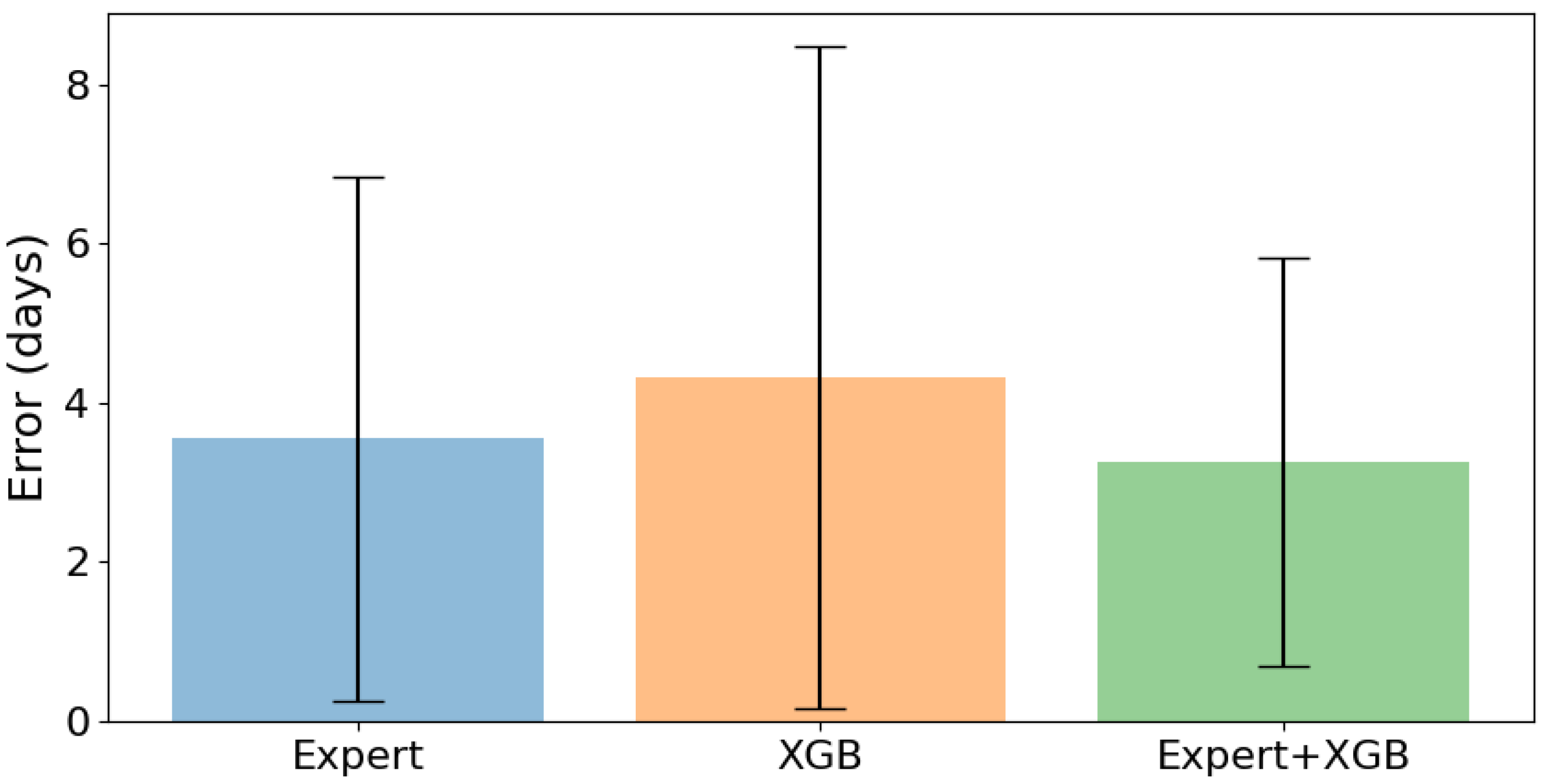
Figure 6 presents a comparison of the mean MSE and its standard deviation for the estimated injury duration between the expert, XGB, and XGB with the expert feature. The figure clearly shows that the combination of XGB and expert feature has the lowest mean MSE and standard deviation compared to a regular XGB and the expert using the LOO test. This indicates that incorporating expert estimations as a feature in the XGB model greatly improves the accuracy and consistency of the injury duration predictions.

To better demonstrate the benefits of adding the expert feature to the XGB model, a more detailed inspection is necessary. Figure 7 shows the estimated recovery duration in days on the x-axis and the true recovery duration in days on the y-axis. It is clear that the XGB model with the expert feature produces more accurate predictions compared to the regular XGB and the expert estimations alone. The XGB model’s predictions are better aligned with the ideal prediction line.

4. Discussion

Injuries can significantly impact the performance of sports teams, causing them to lose games and even suffer financial losses. Head coaches, therefore, need to know how long it takes for a particular injury to heal to make informed decisions. Investing in injury prevention and rehabilitation programs can help reduce the number of days lost due to injury, improve a team’s overall performance, and increase their chances of success. Several studies have demonstrated that lower injury burdens and higher match availability are associated with higher final league rankings, increased points per league match, and success in prestigious tournaments such as the UEFA Champions League or Europa League [7,24,25].

Estimating the duration of recovery after an initial clinical examination is a challenging task, as it depends on various factors such as injury history, age, body type, mental state and more [4]. Additionally, the recovery process may not always follow a predictable pattern, and individual players may recover at different rates [17,26]. This makes accurately predicting RTP time a daunting task, even for experts in the field.

State-of-the-art approaches for estimating the recovery time for a particular injury often involve providing physicians with various recommendations and instructions. However, despite these guidelines, the ultimate decision is usually based on the clinician’s experience with different injury types and their subjective judgment. This decision-making process may be influenced by factors within the soccer club, as well as the clinician’s internal state. Therefore, having a tool that can assist clinicians in their decision-making process could result in more accurate and confident estimates of recovery time.

To date, there has been only one study that attempted to use ML to assess RTP time after hamstring injuries using the MLG-R classification system and the data derived from MR images [14]. The study involved male professional football players from FC Barcelona, and three different ML approaches to assess the importance of each factor of the MLG-R classification system. The results demonstrated that the most important factors to determine the RTP were whether the injury was at the free tendon of the biceps femoris long head or whether it was a grade 3r injury. The study found the MLG-R classification system to be reliable, with excellent results in terms of reliability, prognosis capability and objectivity. However, the performance of the system has not been tested in conjunction with assessments of a medical team. Nonetheless, ML assistance has been already demonstrated in the area of medicine, such as the use of CAD systems to increase radiologists’ diagnosis accuracy [15]. A similar approach can be also applied in the context of clinicians’ estimations regarding RTP in soccer.

This paper presents an approach that enhances the process of recovery estimation by incorporating an expert’s estimations as a feature in the model, in addition to comparing its performance with that of an expert. By integrating human knowledge into the algorithm, we achieve improved performance. This highlights the potential benefits of combining ML methods and human expertise to tackle difficult tasks such as recovery estimation.

One limitation of our study is the relatively small amount of muscle injuries in the dataset. With a longer collection period covering a larger number of soccer clubs and injuries, the algorithm’s performance could increase significantly. The longer period and the amount of data across many seasons might open up an opportunity for expanding the application of the RTP estimator to other injury types, such as bone, joint and tendon. Nonetheless, our dataset reflects a real-world scenario found in many soccer clubs where data are collected over multiple seasons on a single team. Therefore, teams can apply the methods we presented to their own data to improve their injury management processes.

5. Conclusions

In this study, we proposed an ML-based approach for improving the accuracy of predicting the recovery duration of soccer players after an injury. We used three different modeling approaches, namely LR, DT and XGB, to model the recovery duration. We evaluated the performance of these models using several metrics, including MAPE, MSE, RMSE and $R^2$ score and compared it against the expert’s predictions.

The results demonstrated that incorporating the expert’s predictions as a feature greatly improved the performance of all algorithms. XGB achieved the best performance with a mean $R^2$ score of $0.72$, outperforming the expert’s predictions with an $R^2$ score of $0.62$. Our approach demonstrated the potential of combining human knowledge with ML models to improve performance in complex tasks.

These findings have practical implications for soccer practitioners, such as head coaches and medical teams. Accurate recovery duration information for key players could inform tactical decisions and enable coaches to adjust their strategies for upcoming matches. Integrating ML in the RTP decision-making process also adds an additional layer of safety and validity to the medical team’s estimation. Ultimately, this approach can improve the entire RTP process and make it more efficient for planning.

In conclusion, our study demonstrated that ML techniques, in conjunction with human expertise, have the potential to significantly improve the accuracy of predicting recovery duration for injured soccer players. This approach could have important implications for sports medicine, enabling teams to make better decisions regarding the RTP of their players, ultimately improving their performance and reducing the risk of re-injury.

References

- Shrier, I.; Safai, P.; Charland, L. Return to play following injury: Whose decision should it be? Br. J. Sport. Med. 2014, 48, 394–401. [Google Scholar] [CrossRef] [PubMed]
- Matheson, G.O.; Shultz, R.; Bido, J.; Mitten, M.J.; Meeuwisse, W.H.; Shrier, I. Return-to-Play Decisions: Are They the Team Physician’s Responsibility? Clin. J. Sport Med. 2011, 21, 25–30. [Google Scholar] [CrossRef]
- Ekstrand, J.; Krutsch, W.; Spreco, A.; van Zoest, W.; Roberts, C.; Meyer, T.; Bengtsson, H. Time before return to play for the most common injuries in professional football: A 16-year follow-up of the UEFA Elite Club Injury Study. Br. J. Sport. Med. 2019, 54, 421–426. [Google Scholar] [CrossRef] [PubMed]
- Creighton, D.W.; Shrier, I.; Shultz, R.; Meeuwisse, W.H.; Matheson, G.O. Return-to-Play in Sport: A Decision-based Model. Clin. J. Sport Med. 2010, 20, 379–385. [Google Scholar] [CrossRef]
- Snyders, C.; Pyne, D.B.; Sewry, N.; Hull, J.H.; Kaulback, K.; Schwellnus, M. Acute respiratory illness and return to sport: A systematic review and meta-analysis by a subgroup of the IOC consensus on ‘acute respiratory illness in the athlete’. Br. J. Sport. Med. 2021, 56, 223–232. [Google Scholar] [CrossRef] [PubMed]
- Gluckman, T.J.; Bhave, N.M.; Allen, L.A.; Chung, E.H.; Spatz, E.S.; Ammirati, E.; Baggish, A.L.; Bozkurt, B.; Cornwell, W.K.; Harmon, K.G.; et al. 2022 ACC Expert Consensus Decision Pathway on Cardiovascular Sequelae of COVID-19 in Adults: Myocarditis and Other Myocardial Involvement, Post-Acute Sequelae of SARS-CoV-2 Infection, and Return to Play. J. Am. Coll. Cardiol. 2022, 79, 1717–1756. [Google Scholar] [CrossRef]
- Eliakim, E.; Morgulev, E.; Lidor, R.; Meckel, Y. Estimation of injury costs: Financial damage of English Premier League teams’ underachievement due to injuries. BMJ Open Sport Exerc. Med. 2020, 6, e000675. [Google Scholar] [CrossRef]
- Chan, H.P.; Hadjiiski, L.M.; Samala, R.K. Computer-aided diagnosis in the era of deep learning. Med. Phys. 2020, 47. [Google Scholar] [CrossRef]
- Richter, C.; O’Reilly, M.; Delahunt, E. Machine learning in sports science: Challenges and opportunities. Sport. Biomech. 2021, 1–7. [Google Scholar] [CrossRef]
- Castellanos, J.; Phoo, C.P.; Eckner, J.T.; Franco, L.; Broglio, S.P.; McCrea, M.; McAllister, T.; Wiens, J. Predicting Risk of Sport-Related Concussion in Collegiate Athletes and Military Cadets: A Machine Learning Approach Using Baseline Data from the CARE Consortium Study. Sport. Med. 2020, 51, 567–579. [Google Scholar] [CrossRef]
- Eetvelde, H.V.; Mendonça, L.D.; Ley, C.; Seil, R.; Tischer, T. Machine learning methods in sport injury prediction and prevention: A systematic review. J. Exp. Orthop. 2021, 8, 27. [Google Scholar] [CrossRef] [PubMed]
- Majumdar, A.; Bakirov, R.; Hodges, D.; Scott, S.; Rees, T. Machine Learning for Understanding and Predicting Injuries in Football. Sport. Med. Open 2022, 8, 73. [Google Scholar] [CrossRef] [PubMed]
- López-Valenciano, A.; Ayala, F.; Puerta, J.M.; Croix, M.B.A.D.S.; Vera-Garcia, F.J.; Hernández-Sánchez, S.; Ruiz-Pérez, I.; Myer, G.D. A Preventive Model for Muscle Injuries. Med. Sci. Sport. Exerc. 2018, 50, 915–927. [Google Scholar] [CrossRef]
- Valle, X.; Mechó, S.; Alentorn-Geli, E.; Järvinen, T.A.H.; Lempainen, L.; Pruna, R.; Monllau, J.C.; Rodas, G.; Isern-Kebschull, J.; Ghrairi, M.; et al. Return to Play Prediction Accuracy of the MLG-R Classification System for Hamstring Injuries in Football Players: A Machine Learning Approach. Sport. Med. 2022, 52, 2271–2282. [Google Scholar] [CrossRef]
- Winkel, D.J.; Tong, A.; Lou, B.; Kamen, A.; Comaniciu, D.; Disselhorst, J.A.; Rodríguez-Ruiz, A.; Huisman, H.; Szolar, D.; Shabunin, I.; et al. A Novel Deep Learning Based Computer-Aided Diagnosis System Improves the Accuracy and Efficiency of Radiologists in Reading Biparametric Magnetic Resonance Images of the Prostate. Investig. Radiol. 2021, 56, 605–613. [Google Scholar] [CrossRef]
- Grinsztajn, L.; Oyallon, E.; Varoquaux, G. Why do tree-based models still outperform deep learning on typical tabular data? In Proceedings of the 36th Conference on Neural Information Processing Systems (NeurIPS 2022) Track on Datasets and Benchmarks, New Orleans, LA, USA, 28 November–9 December 2022.
- Hallén, A.; Ekstrand, J. Return to play following muscle injuries in professional footballers. J. Sport. Sci. 2014, 32, 1229–1236. [Google Scholar] [CrossRef]
- Pollock, N.; James, S.L.J.; Lee, J.C.; Chakraverty, R. British athletics muscle injury classification: A new grading system. Br. J. Sport. Med. 2014, 48, 1347–1351. [Google Scholar] [CrossRef] [PubMed]
- James, G.; Witten, D.; Hastie, T.; Tibshirani, R. Linear Regression. In Springer Texts in Statistics; Springer: New York, NY, USA, 2021; pp. 59–128. [Google Scholar] [CrossRef]
- Czajkowski, M.; Kretowski, M. The role of decision tree representation in regression problems—An evolutionary perspective. Appl. Soft Comput. 2016, 48, 458–475. [Google Scholar] [CrossRef]
- Chen, T.; Guestrin, C. XGBoost. In Proceedings of the 22nd ACM SIGKDD International Conference on Knowledge Discovery and Data Mining, San Francisco, CA, USA, 13–17 August 2016. [Google Scholar] [CrossRef]
- Giannakas, F.; Troussas, C.; Krouska, A.; Sgouropoulou, C.; Voyiatzis, I. XGBoost and Deep Neural Network Comparison: The Case of Teams’ Performance. In Intelligent Tutoring Systems; Springer International Publishing: Cham, Switzerland, 2021; pp. 343–349. [Google Scholar] [CrossRef]
- Fan, J.; Wang, X.; Wu, L.; Zhou, H.; Zhang, F.; Yu, X.; Lu, X.; Xiang, Y. Comparison of Support Vector Machine and Extreme Gradient Boosting for predicting daily global solar radiation using temperature and precipitation in humid subtropical climates: A case study in China. Energy Convers. Manag. 2018, 164, 102–111. [Google Scholar] [CrossRef]
- Eirale, C.; Tol, J.L.; Farooq, A.; Smiley, F.; Chalabi, H. Low injury rate strongly correlates with team success in Qatari professional football. Br. J. Sport. Med. 2013, 47, 807–808. [Google Scholar] [CrossRef] [PubMed]
- Hägglund, M.; Waldén, M.; Magnusson, H.; Kristenson, K.; Bengtsson, H.; Ekstrand, J. Injuries affect team performance negatively in professional football: An 11-year follow-up of the UEFA Champions League injury study. Br. J. Sport. Med. 2013, 47, 738–742. [Google Scholar] [CrossRef] [PubMed]
- Den Hartigh, R.J.R.; Meerhoff, L.R.A.; Van Yperen, N.W.; Neumann, N.D.; Brauers, J.J.; Frencken, W.G.P.; Emerencia, A.; Hill, Y.; Platvoet, S.; Atzmueller, M.; et al. Resilience in sports: A multidisciplinary, dynamic, and personalized perspective. Int. Rev. Sport Exerc. Psychol. 2022, 1–23. [Google Scholar] [CrossRef]
Figure 1.
Distribution of muscle injuries based on the required recovery time. The vertical dashed line indicates the cut-off threshold of 35 days (5 weeks). Injuries with longer recovery times were excluded from the analysis.
Figure 2.
Distribution of muscle injuries by type, as classified by the BAMIC system. The x-axis denotes different injury types, including classes 1A, 1B, 2B, 3A, and 3B, as well as contusions denoted by C. The y-axis displays the occurrence count for each type of injury.
Figure 3.
A flowchart illustrating the data collection process, feature processing (including data cleaning), hyperparameter tuning and evaluation.
Figure 4.
Estimated versus true recovery duration for LR (blue circles), DT (green asterisks) and XGB (orange triangles) algorithms. The diagonal black dotted line represents ideal estimations, while green and red backgrounds indicate that the recovery was faster or slower than estimated, respectively.
Figure 5.
Comparison of the estimations made by the expert (blue circles) with the predictions of the best performing algorithm, XGB (orange asterisks). The black dotted line shows ideal predictions, while green and red backgrounds indicate cases where the recovery was faster or slower than expected.
Figure 6.
A bar plot showing the mean MSE of expert’s estimations (blue bars), XGB model (orange bars) and XGB model with the inclusion of expert’s predictions as a feature (green bars). The black lines on each bar indicate the corresponding standard deviation of the MSE.
Figure 7.
Visualization of the estimations made by the expert (blue circles), and XGB with the inclusion of the expert’s predictions as a feature (orange asterisks). The black dotted line shows ideal predictions, while green and red backgrounds indicate cases where the recovery was faster or slower than expected.