Retrospective-Based Deep Q-Learning Method for Autonomous Pathfinding in Three-Dimensional Curved Surface Terrain

Abstract

Path planning in complex environments remains a challenging task for unmanned vehicles. In this paper, we propose a decoupled path-planning algorithm with the help of a deep reinforcement learning algorithm that separates the evaluation of paths from the planning algorithm to facilitate unmanned vehicles in real-time consideration of environmental factors. We use a 3D surface map to represent the path cost, where the elevation information represents the integrated cost. The peaks function simulates the path cost, which is processed and used as the algorithm’s input. Furthermore, we improved the double deep Q-learning algorithm (DDQL), called retrospective-double DDQL (R-DDQL), to improve the algorithm’s performance. R-DDQL utilizes global information and incorporates a retrospective mechanism that employs fuzzy logic to evaluate the quality of selected actions and identify better states for inclusion in the memory. Our simulation studies show that the proposed R-DDQL algorithm has better training speed and stability compared to the deep Q-learning algorithm and double deep Q-learning algorithm. We demonstrate the effectiveness of the R-DDQL algorithm under both static and dynamic tasks.

1. Introduction

In recent years, the utilization of unmanned ground vehicles (UGVs) has become increasingly prevalent in a variety of applications, including transportation, investigation, and detection [1,2,3]. However, as the operational environment of UGVs becomes more complex, a number of challenging surface-path problems have emerged [4], such as field rescue and warfare path planning. Achieving accurate and efficient path planning is essential for UGVs to effectively execute their designated tasks. Despite advancements in autonomous UGV technology, path planning remains a challenging task due to the multifaceted and intricate factors influencing path selection in diverse environments, including information accuracy, cost considerations, and risk assessment.

Traditional path-planning studies typically focus on obstacle avoidance while minimizing distance, using two-dimensional maps to identify feasible and impassable areas, while disregarding terrain height information and other costs. In practice, UGVs should consider terrain height information and other costs when deciding on a path. For example, Ma et al. [5] used terrain complexity to calculate the optimal strategy for autonomous underwater vehicles. Cai et al. [6] considered localization uncertainty, collision risk, and travel costs to the target area in their path-selection algorithm. Ji et al. [7] integrated road roughness and path length to select the optimal path. Nevertheless, most current algorithms combine the multidimensional cost with varying weights, necessitating adjustments to the algorithm and weights when the environment changes, which can be difficult to handle.

To address the above problems, we propose a new decoupled model for path planning with path cost, which divides the path-planning model into two parts: the cost map and the main path-planning algorithm. Specifically, the multidimensional path-cost fusion is represented as height information in the 3D map. The path-planning master algorithm can find the best path using input from the previous part. It only adjusts the 3D map without changing the algorithm parameters when the environment changes. The main advantage is that the factors and weights of the path cost can be easily changed even if the UGV is in motion. This approach can be applied to the autonomous navigation of UGVs, where cost factors often fluctuate, such as when the environment cost factors change during robot detection or when the driving path requires a more aggressive or conservative strategy. It has the potential to enhance the efficiency and accuracy of path planning. However, this requires the main algorithm to be adaptable and efficient in processing.

Reinforcement learning (RL) maximizes the cumulative rewards through trial-and-error interactions with the environment, enabling agents to learn the best policy autonomously. Q-learning, as a popular model-free reinforcement learning algorithm, has been widely used in various fields [8]. For example, Liu et al. [9] designed a path-planning model based on Q-learning that ensures obstacle avoidance and energy savings of underwater robots. Babu et al. [10] used Q-learning to propose an automatic path-planning method that uses a camera to detect the location of obstacles and avoid them. However, the limitation of the Q-learning algorithm is that it is difficult to deal with the high-dimensional state required in this study.

The deep Q-learning (DQL) method overcomes this limitation by combining deep learning and Q-learning. Deep learning enhances the feature extraction of the environment and realizes the fitting of an action value and environmental state, while Q-learning completes the mapping from state to action through the reward function and decides according to the output of deep neural network and exploration strategies [11]. As a result, high-dimensional states can be dealt with. Pictures are the input of states of DQL, and the output is the Q value of each action. Agents using the DQL algorithm can achieve human-level performance when playing many Atari games [12]. This approach has been widely used in robotics. For instance, [13] used DQL to solve the combinational optimization problem of a robot patrol path, and the result was better than that of the traditional algorithm. In [14], the DQL algorithm was used to solve the problem of autonomous path planning for UAVs under potential threats. DQL can better meet the demands of UGV path planning [15].

Despite the success of deep Q-learning (DQL) in solving complex decision-making problems, it still faces several limitations such as low sampling efficiency, slow convergence speed, and poor stability. To address these issues, many researchers have proposed various techniques to improve the training speed, accuracy, and stability of DQL. For instance, Wu et al. [16] proposed an effective inert training method to enhance the training efficiency and stability of DQL. Similarly, Van et al. [17], introduced the double deep Q-learning (DDQL) method, which decomposes the action evaluation to prevent overestimation [14].

• In this paper, we aim to improve the stability and convergence speed of the algorithm in a novel way by incorporating a retrospective mechanism to enhance the DQL during training. Specifically, we leverage fuzzy logic methods to guide the DQL in finding the optimal solution when needed, thus improving the training process to some extent. We assume that the global terrain information has been obtained. The primary contributions of our work are as follows: We propose a decoupled path-planning algorithm with multidimensional path costs, which provides greater advantages when the path-cost factors change.
• We propose a three-dimensional map information-processing program that can rapidly convert three-dimensional terrain information into the image data required by DDQL.
• We introduce a novel training method that improves the performance and stability of DDQL. Specifically, we integrate fuzzy logic as a retrospective mechanism into the training process.

The structure of this paper is as follows: In Section 2, we introduce the system framework of our proposed methods. Section 3 provides detailed information about the proposed framework. Section 4 presents the experimental setup and results. Finally, in Section 5, we conclude the paper and discuss possible future research directions.

2. System Framework

2.1. DQL Algorithm and DDQL Algorithm

Double deep Q-learning (DDQL) is an improved version of deep Q-Learning (DQL) that overcomes the overestimation problem. In this paper, we aim to further enhance the stability and convergence speed of the DDQL algorithm. DDQL serves as the foundation for our work, and we introduce a refined version called R-DDQL. While DQL employs the same neural network for both action selection and action evaluation, DDQL separates the two processes, thus avoiding the issue of overestimation effectively. Specifically, DDQL decomposes the action selected from the action evaluation, which results in an improved accuracy of the action-value function. According to reference [17], the target Q values of DQL and DDQL are as follows:

$$y_t^{DQL}=r_{t+1}+\gamma Q(s_{t+1},\underset{a^{\prime }}{\arg \max }Q(s_{t+1},a^{\prime };{\theta }^{-});{\theta }^{-})$$

(1)

$$y_t^{DDQL}=r_{t+1}+\gamma Q(s_{t+1},\underset{a^{\prime }}{\arg \max }Q(s_{t+1},a^{\prime };\theta );{\theta }^{-})$$

(2)

where $y_t^{DQL}$ is the target Q-value of DQL, $y_t^{DDQL}$ is the target Q-value of DDQL, $\theta$ is the parameter of the online network, and ${\theta }^{-}$ is the parameter of the target network. The two networks use the same structure. The target network is a lagging version of the online network.

2.2. DQL Algorithm and DDQL Algorithm

In this section, we will introduce the method framework and the functionality of each component. The entire model is divided into three parts: 3D terrain processing, action selection, and state collection, as illustrated in Figure 1.

The 3D terrain-processing module is responsible for converting the geographic information into image data that can be used by the model. The image data include the location of the agent, the location of the target, and the terrain information. The action-selection module employs heuristic knowledge or a neural network to select the next action. The retrospective mechanism analyzes the quality of the action chosen by the action-selection module and determines if there exists a better alternative. The state-collection module combines the next state obtained from the action-selection module with the state obtained from the retrospective mechanism to obtain a comprehensive state. These states will be utilized to train the neural network until a satisfactory strategy is obtained.

Overall, the 3D terrain-processing module converts geographic information into a suitable format for the model to use, the action-selection module selects the next action using either heuristic knowledge or a neural network, and the retrospective mechanism analyzes the quality of the selected action to potentially identify a better alternative. The state-collection module combines the states from the previous two modules and is used to train the neural network to optimize the strategy.

3. DDQL with Retrospective Mechanism for Path Planning

In this section, we provide a detailed description of our proposed method. Specifically, Section 3.1 outlines the 3D terrain-processing module, which serves as the foundation for roadless path planning in curved terrain. In Section 3.2, we delve into the Markov decision process (MDP) that we employ. Subsequently, Section 3.3 elaborates on the retrospective mechanism, and Section 3.4 illustrates the action-selection policy that we adopt. Finally, in Section 3.5, we present other pertinent details that are relevant to our approach.

3.1. 3D Terrain Processing

The 3D terrain-processing module serves as the foundation for roadless path planning in curved terrain, providing the necessary means to reduce the data scale and model complexity. This module plays an indispensable role in addressing the path-planning problem under 3D terrain conditions.

In this paper, we consider the height of the terrain as the cost incurred by the agent to traverse it. We draw an analogy between the agent and an off-road vehicle in the desert, which must carefully choose the lowest dune to climb over in order to reach its destination. Accordingly, each height value is deemed significant, and we do not treat all points above the ground level as obstacles, which is a common approach adopted in traditional path-planning algorithms.

3.1.1. 3D Terrain Rasterization

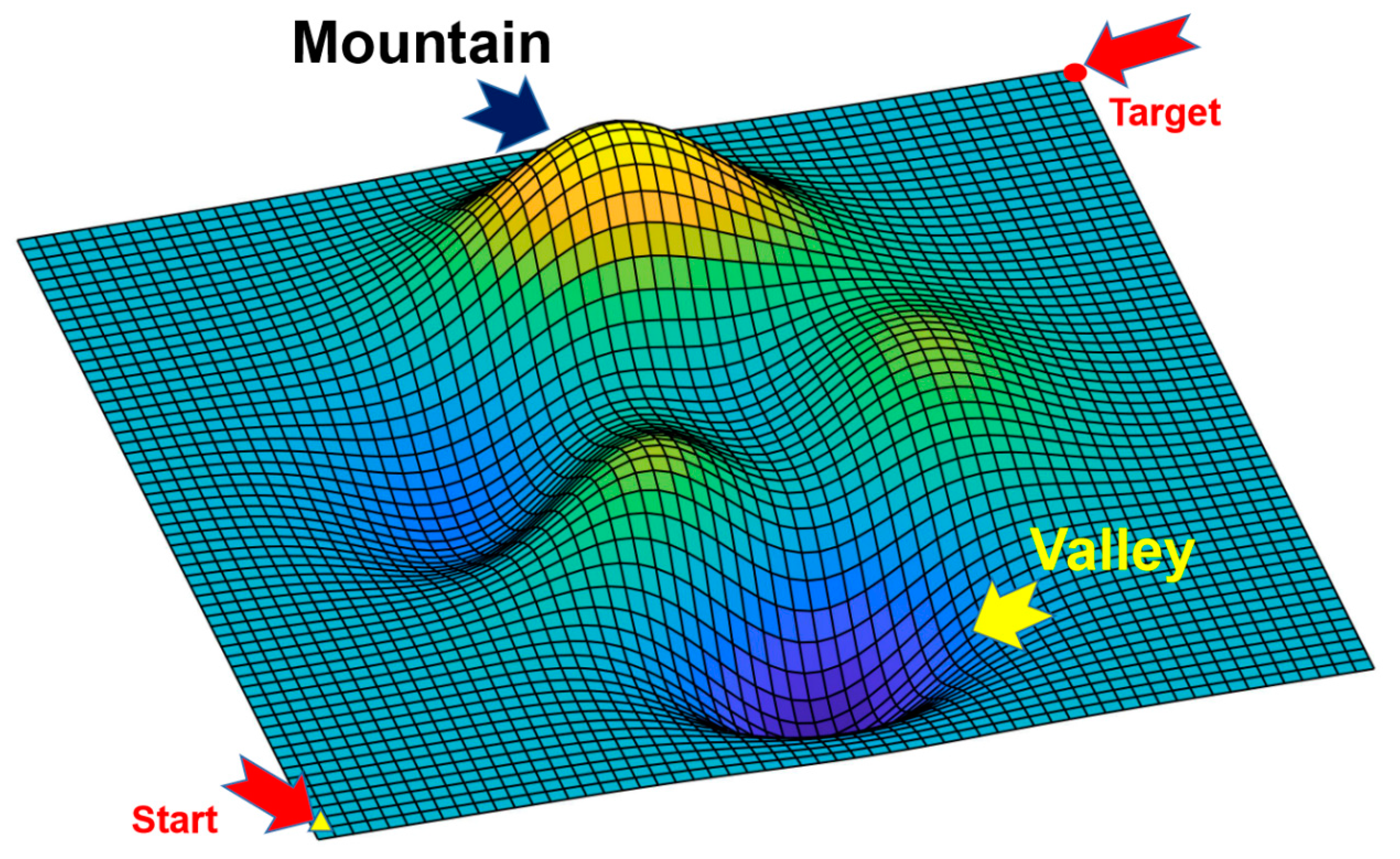
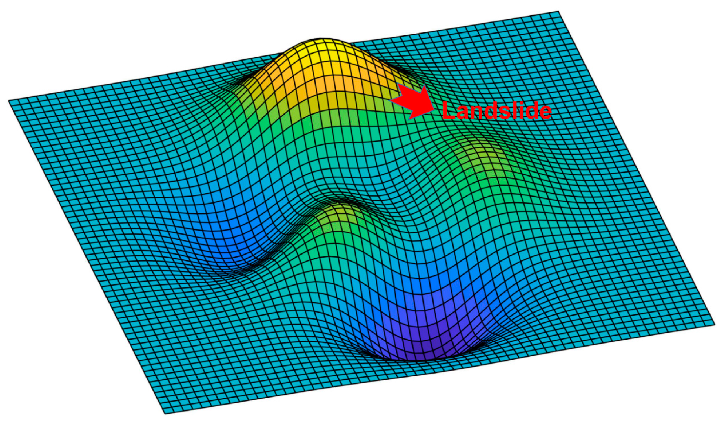
Similar to the surface maps in the literature [4], this paper employs the peaks function to generate a 3D terrain model for path planning, as depicted in Figure 2. The peaks function is defined as follows:

$$\mathrm{H}=3{(1-x)}^2{e}^{-x^2-{(y+1)}^2}-10\left(\frac{x}{5}-x^3-y^5\right)e^{-x^2-y^2}-\frac{1}{3}{e}^{-{\left(x+1\right)}^2-y^2}$$

(3)

where H is the height of the terrain information; $x$ and $y$ are the values of the coordinate axis $x$ and $y$, respectively, which are within the range of −3 to +3.

Since a large amount of 3D surface data can impede the model calculations, it is necessary to rasterize the terrain by discarding some extraneous data to simplify the 3D map model. To this end, this paper converts the terrain information into a 3D raster map through the following steps:

• Step 1: Determine the density of sampling points in the projection plane.
• Step 2: Calculate the height value of each sampling point.
• Step 3: Draw the three-dimensional raster map.

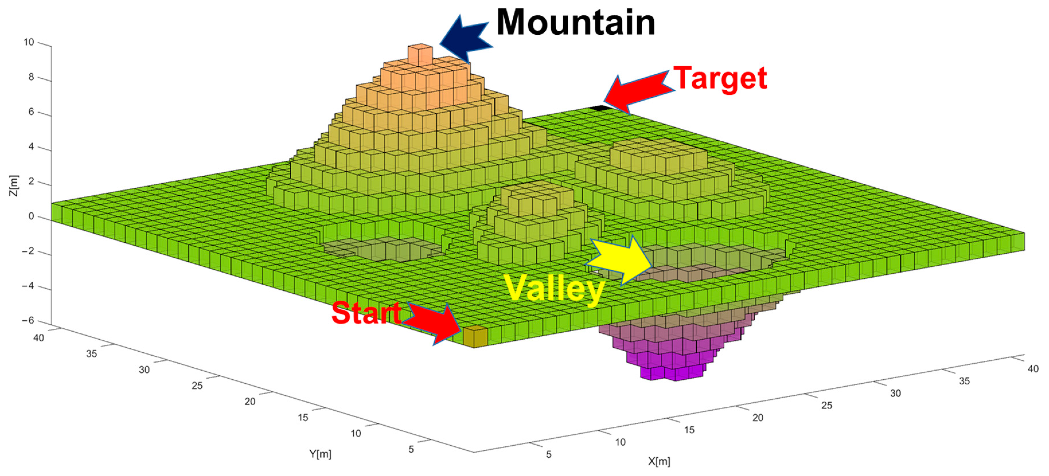
Using this approach, maps with a density of 41 × 41 have been generated (see Figure 3).

In Figure 3, the grid with zero height is considered the horizontal plane, and it is designated in green. The region above the horizontal plane becomes slightly reddish as the height increases, while the part below the horizontal plane gradually deepens in color as the height decreases. The red grid denotes the starting point, while the black grid represents the destination.

3.1.2. Converting 3D Raster Map to 2D Map

Two-dimensional maps are more suitable for inputting reinforcement learning models than three-dimensional maps. Hence, this paper converts the three-dimensional raster map to a two-dimensional map while preserving the height information. Drawing on the method used in [14], each height value H is converted to a pixel value of the color channel using the formula:

$$V=V_{\min }+\frac{H-H_{\min }}{H_{\max }-H_{\min }}(V_{\max }-V_{\min })$$

(4)

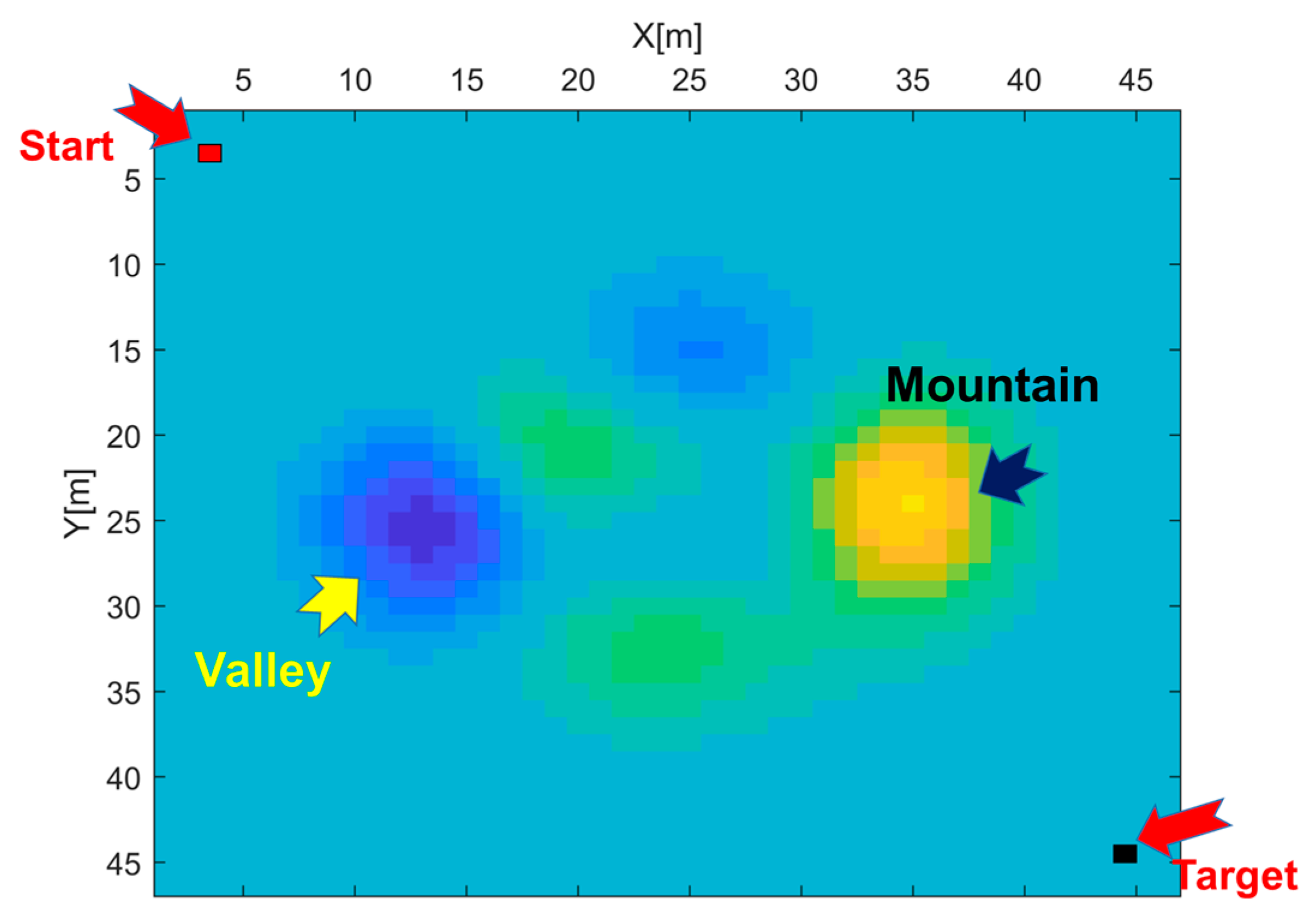
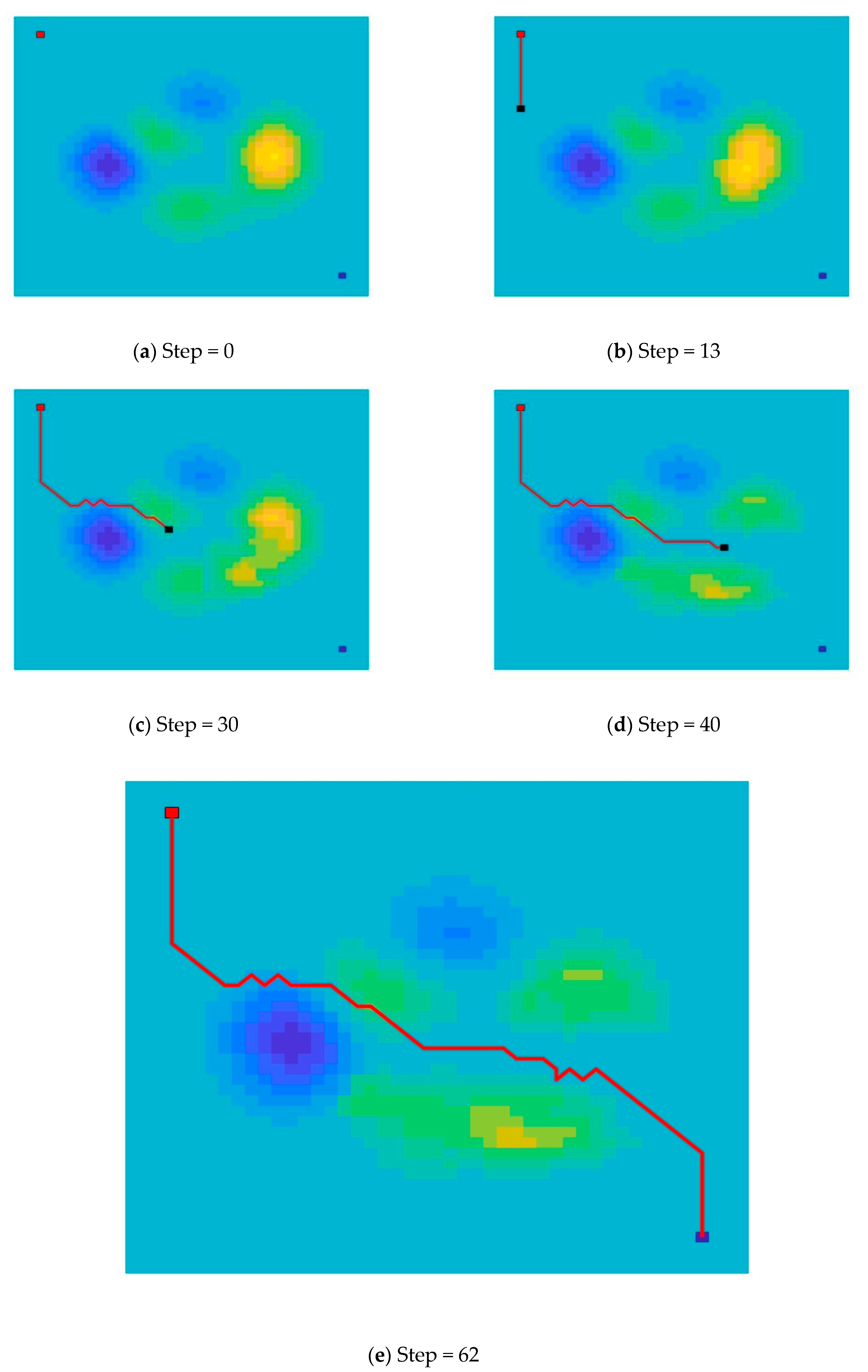
Here, $V_{\max }$ and $V_{\min }$ are the maximum and minimum pixel values for a color channel, respectively; $H_{\max }$ and $H_{\min }$ are the maximum and minimum height values, respectively. The resulting 2D map is shown in Figure 4.

In Figure 4, the red rectangle denotes the starting position, and the black rectangle represents the target area. The mission is deemed successful if the agent reaches the target. The yellow area and dark area represent hillsides and pools, respectively. To input the picture into the model when the agent crosses the map boundary, we fill an area with a width of 3 around the two-dimensional map. Thus, the size of the two-dimensional map becomes 47 × 47, which is used as the input to the model.

3.2. MDP Model

3.2.1. State

In this study, the state of the agent is composed of three key pieces of information, namely, the agent’s position, the target position, and the terrain information. These pieces of information are synthesized into an image, which serves as the input to the deep Q-network (DQN) algorithm, as depicted in Figure 4.

3.2.2. Action

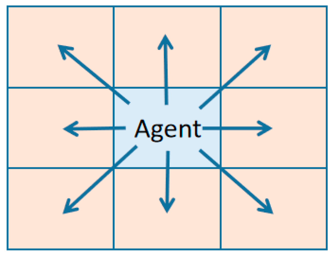
The agent is allowed to move freely within the eight surrounding grids, as illustrated in Figure 5.

3.2.3. Reward

The reward function will be used to judge whether the action chosen by the agent in the current state is good or bad in reinforcement learning. Based on these reward values, the agent tends to the best strategy in its interaction with the environment.

The reward function is used to evaluate the agent’s performance in the current state and, accordingly, guide its behavior towards the optimal strategy. During the training process, the reward function is defined as shown in

Table 1. Reward function.

State	Reward Value
Reach the target location	+200
Outside the map boundary data	−50
Climbing over obstacles	$-\left|H(s^{\prime })\right|$
Otherwise	−0.5

. If the agent reaches the target location, it obtains a high positive reward (+200). Conversely, if it moves outside the map boundary, it receives a penalty in the form of a negative reward (−50). In addition, a negative reward ($-\left|H(s^{\prime })\right|$) is assigned for climbing over obstacles to encourage the agent to choose a flatter path. Finally, a small negative reward (−0.5) is given for each step taken by the agent to motivate it to reach the target as quickly as possible. In summary, the reward function is designed to encourage the agent to navigate towards the target while avoiding obstacles and staying within the map boundary.

3.3. Retrospective Mechanism

In human learning, retrospective evaluation and summarization play crucial roles in significantly enhancing learning efficiency. In this paper, we innovatively propose that a retrospective mechanism can be employed to simulate this behavior and improve the performance of reinforcement learning.

Fuzzy logic methods are a widely-used tool in the field of robotics [18,19,20]. In this study, a fuzzy logic design has been employed for the retrospective mechanism to improve the performance of DDQL. The primary objective of the backtracking mechanism is to evaluate the action score and select actions based on the state. To this end, we have utilized the Mamdani fuzzy logic approach, which has been well-documented in the literature [21].

The application of fuzzy logic methods in robotics is beneficial because it enables the creation of more sophisticated algorithms that can better model and handle the uncertainties that are inherent in robotic systems. The use of fuzzy logic in the retrospective mechanism allows for the evaluation of action scores in a more nuanced and context-dependent manner, which can lead to more effective action selection.

The Mamdani fuzzy logic approach, in particular, is well-suited for this task because it can accommodate a wide range of input variables and output values and can handle non-linear relationships between them [22]. This approach allows for the development of complex inference rules that can capture the intricacies of the task at hand. By using this approach, we can evaluate the actions based on a range of factors and select the best action based on an overall score that takes into account these different factors.

3.3.1. Fuzzy Logic Structure

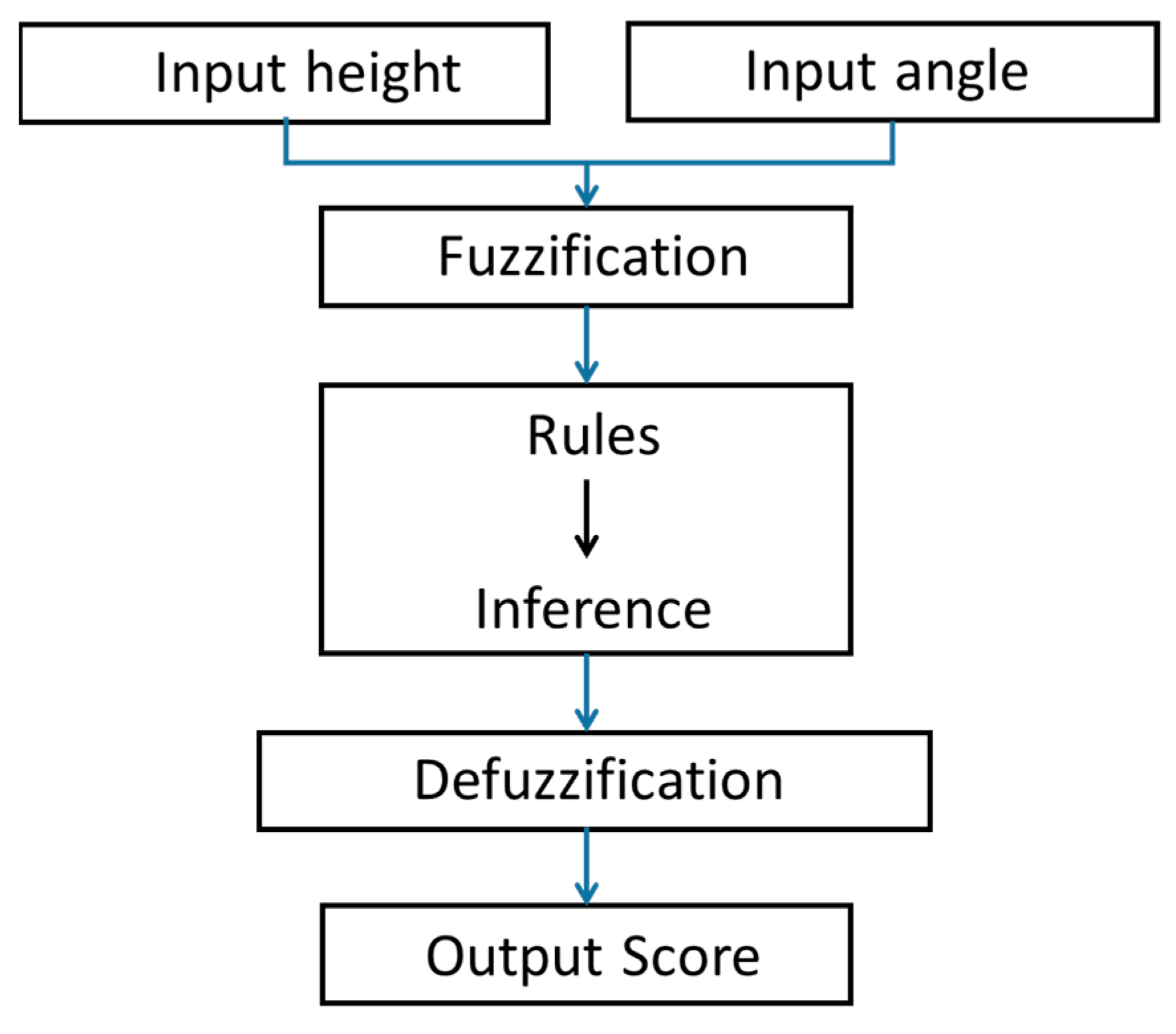
The fuzzy logic structure consists of two input variables: first, the angle ($\theta$) between the selected action and the target point; second, the maximum height value ($H$) within a certain range (3 steps) in the selected direction. The output is the score of the selected action. The process is illustrated in Figure 6.

3.3.2. Fuzzification

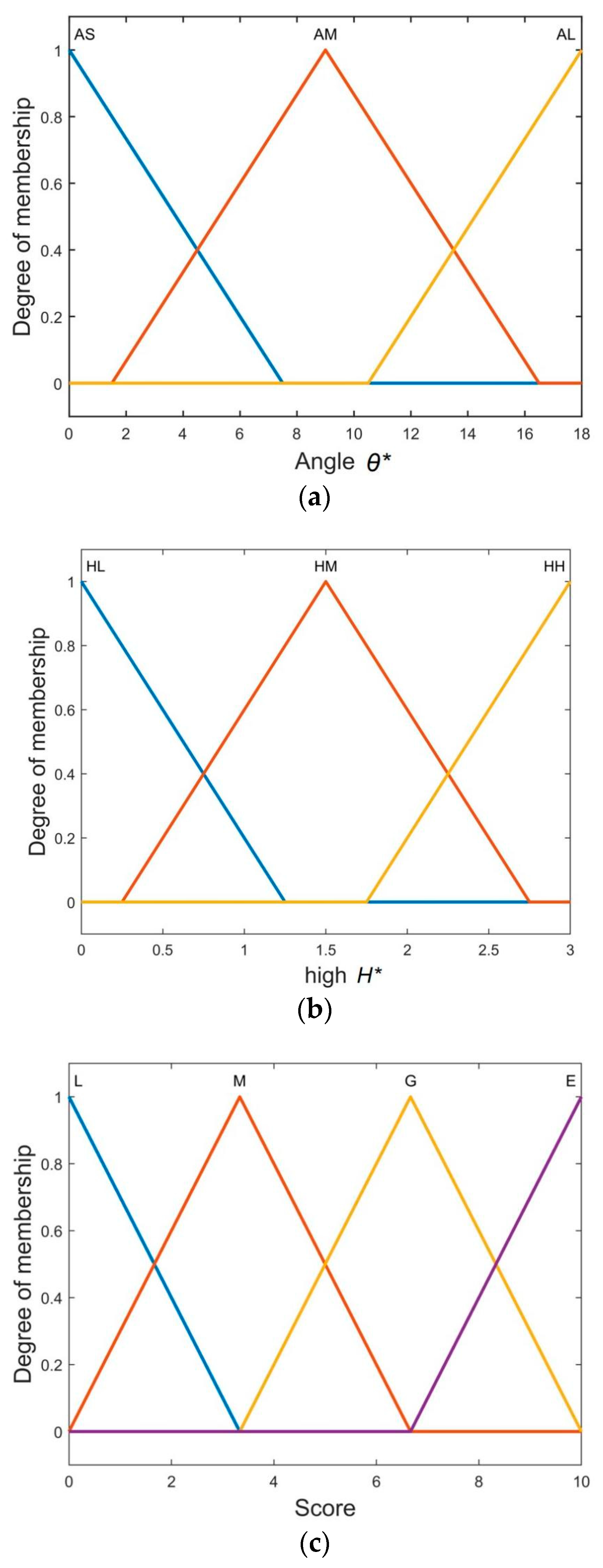
Using the linearization processing method, the fuzzy subset of the angle variable is partitioned into {small, medium, large}, which are expressed as {AS, AM, AL}. The actual angle range is from 0 to 180 degrees, and the model input range is from 0 to 18. The linear transformation is depicted in Formula (5), and the membership function of ${\theta }^{*}$ is shown in Figure 7a.

$${\theta }^{*}=k_1\theta$$

(5)

where $\theta$ is the actual angle and $k_1=0.1$ is the scale factor.

The fuzzy subset of the height variable is divided into {low, medium, high}, expressed as {HL, HM, HH}. The range of actual height $H$ is from−5 to +8, and the formula $H^{*}=\min (\left|H\right|,3)$ is used for processing. Therefore, the range of input $H^{*}$ is from 0 to 3. Its membership function is shown in Figure 7b.

The output variable is the score, denoted by S. The fuzzy subset of S is divided into {low, medium, good, excellent}, simplified to {L, M, G, E}, The higher the score, the better the selected action. The membership function of the score is shown in Figure 7c.

3.3.3. Other Details for Fuzzy Logic

Fuzzy control rules consist of a set of multiple conditional statements that allow for effective control of the agent’s behavior. When the agent has a large angle to the target point or climbs over obstacles, the score for these actions is low. Two qualitative input variables $IN1$ and $IN2$ and a qualitative output variable $O$ are specified, and fuzzy rules are defined accordingly, for example:

• Rule 1: If ($IN1$ is AS) and ($IN2$ is HL), then ($O$ is E)
• Rule 9: If ($IN1$ is AL) and ($IN2$ is HH), then ($O$ is L)

These rules are listed and stored in a database for future reference (see

Table 2. Fuzzy rules.

	IN1	AS	AM	AL
IN2
HL		R1: E	R4: G	R7: M
HM		R2: G	R5: G	R8: L
HH		R3: M	R6: L	R9: L

). The symbols in the table represent the output variable resulting from the two input variables of each corresponding rule. For instance, R4: G in Table 2 can be interpreted as rule 4: If ($IN1$ is AM) and ($IN2$ is HL), then ($O$ is G).

This study employs the Mamdani inference system for fuzzy inference, which comprises fuzzy operator application, method of implication, and aggregation [21].

• Fuzzy operator application: Generally, a fuzzy logical operator is of two types: one is OR and the other is AND. This study uses the AND operator.
• Method of implication: Generally, Mamdani systems use the AND implication method. Hence, AND implication method is used in this paper.
• Aggregation: The input of the aggregation is the list of output functions returned by the previous implication process for each rule. The output of the aggregation process is a single fuzzy set for each output variable.

The center of gravity method is adopted to defuzzify and generate the final output of fuzzy inference, as depicted in Formula (6).

$$u=\frac{{\displaystyle \int u_N(x)xdx}}{{\displaystyle \int u_N(x)dx}}$$

(6)

where $u_N(x)$ represents the function value corresponding to the aggregation part, $x$ is the abscissa value corresponding to $u_N(x)$, and $u$ is the center of the area on the abscissa.

3.3.4. Output of Fuzzy Logic System

When the agent is in a certain position (such as the black grid in Figure 8) in the map, the retrospective mechanism will output the scores of the surrounding positions, as shown in Figure 8.

The retrospective mechanism assigns a higher score to a grid that is closer to the target and free of obstacles. The state with the highest score is denoted as $s^{″}$, and the action required to reach the grid with the next-highest score is designated as $a^{\prime }$.

3.4. Action-Selection Policy

Building upon [23], we introduce heuristic search rules into the action-selection policy to enhance the training efficiency and minimize blind explorations. Specifically, when the agent randomly selects an action with a probability of $\epsilon$, it is bound by certain rules to ensure that it prioritizes actions that approach the target and chooses actions with low obstacles. In cases where multiple choices exist in the same situation, the agent will make a random selection. These heuristic rules are expected to enhance the agent’s ability to navigate through complex environments. The pseudo-code for the action selection policy is shown in Algorithm 1.

Algorithm 1: Action-selection policy

Generating d randomly, d ∈ (0,1) If d > ε   $a=argmax\left(Q\left(s,a_i\right)\right)$ else   $\mathrm{Pr}e\text{\_}a=Closer\text{-}target\left(eightaction\right)$   $\mathrm{Pr}e\text{\_}b=Smoother\left(\mathrm{Pr}e\text{\_}a\right)$   $a=random\left(\mathrm{Pr}e\text{\_}b\right)$ End if

3.5. Other Details

3.5.1. R-DDQL Network Structure

DQL, utilizing a convolutional neural network (CNN), has demonstrated exceptional performance in game-playing and image-recognition applications [24,25,26]. In order to further improve its performance, this paper proposes to replace the BP neural network in the general deep Q-network with a CNN. Specifically, a CNN is employed as the neural network for DDQL, referred to as DDQN. For comparison, R-DDQL also uses the same CNN architecture, which is denoted as R-DDQN. Figure 9 illustrates the structure of the CNN, where the input is the image in Figure 4 and the output is the Q-value of the eight actions. The CNN processes the image in the following manner: First, the image is convolved by a filter and a feature map is generated through a nonlinear activation function $relu(x)$, defined as $max\left(0,x\right)$. Subsequently, maximum pooling is executed, followed by a series of similar operations to obtain a fully connected layer with a size of 1 × 8.

Table 3. Layer parameters of the convolutional neural network.

Name	Value
Input layer	47 × 47 × 3
Convolution layer	3 × 3 × 40
Feature map after convolution	24 × 24 × 40
Feature map after pooling	12 × 12 × 40
Convolution layer	3 × 3 × 50
Feature map after the second convolution	10 × 10 × 40
Full connection layer	1 × 40
Output layer	1 × 8

summarizes the parameters of each layer.

3.5.2. Overall Training Framework

In this article, we adopt a retrospective mechanism to improve the stability and performance of the DDQL model. Algorithm 2 is the overall training framework of the proposed model.

Algorithm 2: Overall training framework

1. Initialize memory D to capacity N

2. The random weight θ is used to initialize the evaluation network

3. Let ${\theta }^{-}=\theta$ initialize the target network which is used to calculate target Q-value

4. For iteration = 1, Max episodes do

Initialize step and the first state s0

While state ~ == target state && step < = M

Choose action a by Algorithm 1

In the simulator, action a is executed; reward $R$ and state $s^{\prime }$ are observed.

Store the data (s, a, s′) in memory D

Obtain a’, s’’ using retrospective mechanism as shown in Section 3.3

Store the data (s, a’, s″) in memory D

Set $s=s^{\prime }$, step++

Target network weight is updated every 3C step, that is, ${\theta }^{-}=\theta$

Every C step, do

A mini-batch-size data is randomly sampled from memory D and expressed as $\left(s_j,a_j,R,{s_j}^{\prime }\right)$

Perform gradient-descent algorithm once then update the network parameter by $\theta =\theta +\Delta \theta$

End while

End for

4. Experiments and Analysis

In this section, we apply the R-DDQL algorithm proposed in Section 3 to solve the problem of 3D path planning and compare its performance with that of the DDQL and DQL algorithms. For the purpose of comparison, all three algorithms are assigned the same parameters, except that R-DDQL incorporates the retrospective mechanism proposed in Section 3.4. The comparison is divided into two parts: the training phase and the training results.

4.1. Parameter Setting

All models adopt the same parameters, which are presented in

Table 4. The parameters of the neural network.

Parameter	Value
Network learning rate	0.0001
Discount factor	0.9
Memory capacity D	20,000
Greed factor $\epsilon$	$0.001\ast IT$
Max steps M	200
$Pre\text{\_}episodes$	10
Max episodes	2000
Mini-batch size	400

. The maximum number of steps, denoted by M, is set to 200, indicating that if the agent fails to reach the target within 200 steps, the episode will terminate, and the next episode will begin. Moreover, the value of the greedy factor, denoted by ε, is initially set to $0.001\ast IT$ (where $IT$ is the number of episodes at that moment). This means that after 1000 episodes, the heuristic rules are disabled, and the agent continues to explore according to the greedy algorithm for another 1000 episodes. In the pre-training phase, the model is executed ten times to fill the memory, and thus the initial value of $Pre\text{\_}episodes$ is set to 10. Therefore, all three algorithms are trained for 2010 episodes. However, since the model is not trained during the pre-training phase, it is not included in the total training count in this study.

4.2. Training-Phase Comparison

The figure depicting the cumulative rewards obtained during the training of the three algorithms is presented in Figure 10.

The cumulative reward curves of the three algorithms during training are presented in Figure 10. As can be observed, after 1000 episodes (line 1), the heuristic search rules are disabled, and all three algorithms experience a sharp decrease in the cumulative rewards. However, R-DDQL achieves higher rewards at a faster rate. Specifically, R-DDQL tends to converge after line 2 (at 1406 episodes) and remains stable after line 3 (at 1602 episodes), whereas the remaining two algorithms start to converge after line 4 and do not stabilize before the end of the training. Therefore, R-DDQL exhibits higher stability compared to DDQL and DQL, indicating that the proposed retrospective mechanism can mitigate the overestimation issue and enhance the training stability.

4.3. Training Results Comparison

The paths of the three algorithms are presented in Figure 11, where the details of the image are consistent with those introduced in Section 3.1. Specifically, the red grid in the upper-left corner of the image denotes the starting point of path planning, while the blue grid in the lower-right corner represents the target area. Moreover, the black line indicates the DQL, the blue line indicates the path of DDQL, whereas the red line illustrates the path of R-DDQL. Notably, all three algorithms select the option to traverse over the lowest slope to reach the end, instead of circumventing around the side. However, the DQL and DDQL algorithms manifest hesitation before opting to enter the mountainous area (as indicated by the black arrow). In contrast, the R-DDQN algorithm is notably smoother than DQL and DDQL. The comparative analysis results are provided in

Table 5. DDQL and R-DDQL path comparison.

	DQL	DDQL	R-DDQL
Steps	59	56	47
Turns	29	25	15
Cumulative reward	156.5	162	170.5

.

Table 5 provides a comprehensive quantitative comparison of the path-planning performance of the three algorithms. As shown in the table, the path generated by DQL requires 59 steps to reach the target and involves 29 turns, resulting in a cumulative reward of 156.5. In contrast, the path generated by DDQL requires only 56 steps to reach the target and involves 25 turns, accumulating a reward of 162. However, the R-DDQL algorithm stands out with a superior performance, reaching the target in only 47 steps and involving only 15 turns, while accumulating a higher reward of 170.5. Notably, DDQL significantly outperforms DQL, while R-DDQL outperforms DDQL in terms of the number of steps taken, the number of turns involved, and the cumulative reward, with improvements of 16%, 40%, and 5.2%, respectively. These results demonstrate that while all three methods can plan paths, R-DDQL is optimal. In order to further assess the efficacy of the R-DDQL algorithm in typical scenarios, we conducted simulation experiments on five additional maps. The corresponding data-comparison plots are presented in Figure 12. Our results clearly demonstrate that the R-DDQL algorithm outperforms both the DDQL and DQL algorithms. Specifically, across all five experiments, R-DDQL exhibited a superior step performance by 32.5%, steering performance by 45%, and cumulative rewards by 69.4% compared to DQL. Similarly, when compared to DDQL, R-DDQL achieved a 21.3% improvement in step performance, a 48% improvement in steering performance, and a 58% improvement in cumulative rewards.

4.4. Performance of R-DDQN in a Dynamic Environment

In order to demonstrate the effectiveness of our proposed method in dynamic scenarios, we conducted a dynamic path-planning experiment where the mountain collapses while the agent is navigating through the path. As shown in Figure 13, the highest mountain collapses and obstructs the canyon that the agent had previously passed through. We trained the R-DDQL model, which was previously trained under static conditions, for an additional 2000 episodes under this dynamic scenario. The training parameters remained consistent with the previous training.

Figure 14 displays the performance of R-DDQL in this dynamic scenario. Remarkably, the agent successfully selects a flat road from the collapsed terrain instead of following the previous path. This demonstrates that our proposed method can still perform well in dynamic environments.

5. Discussion

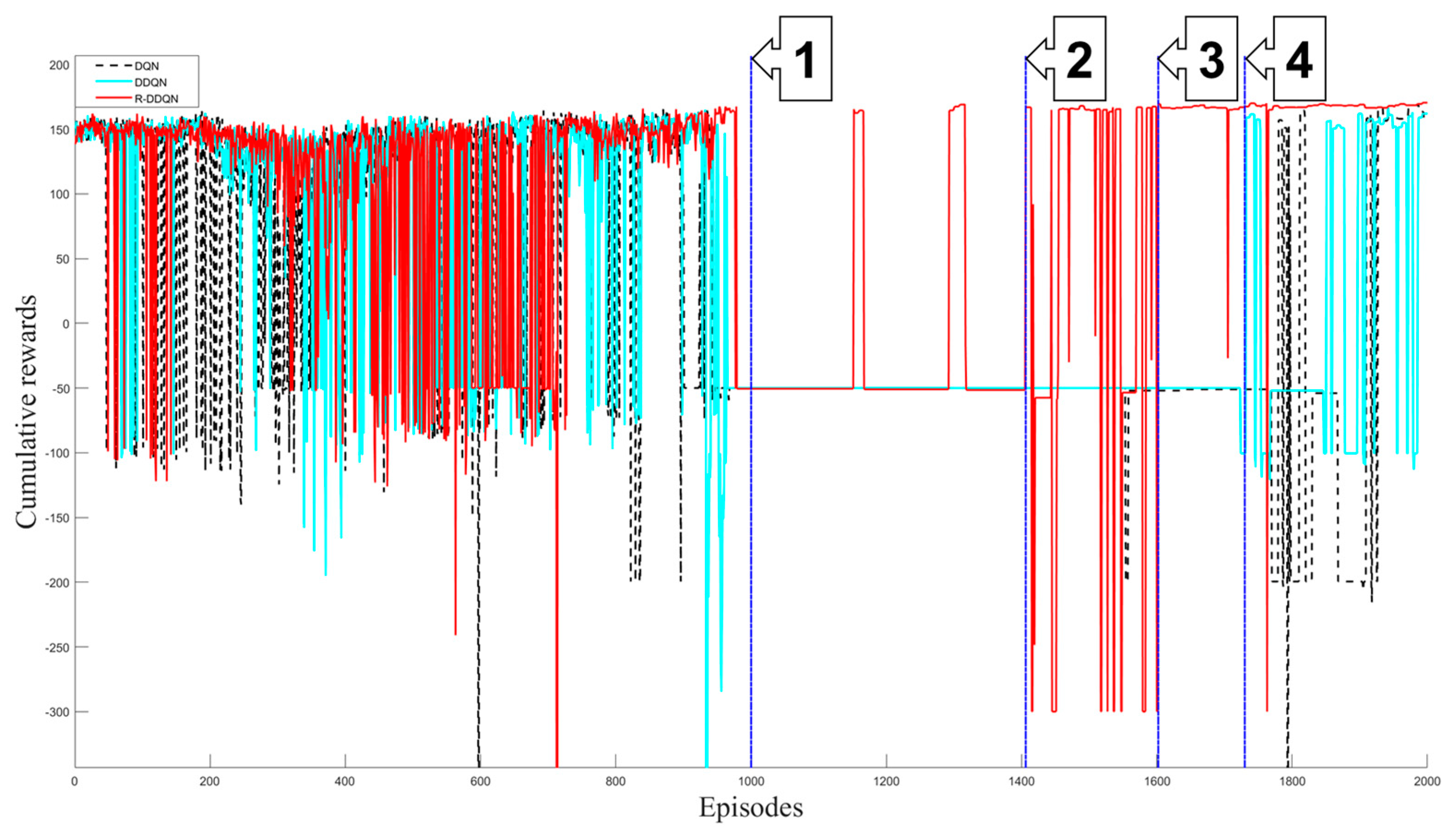
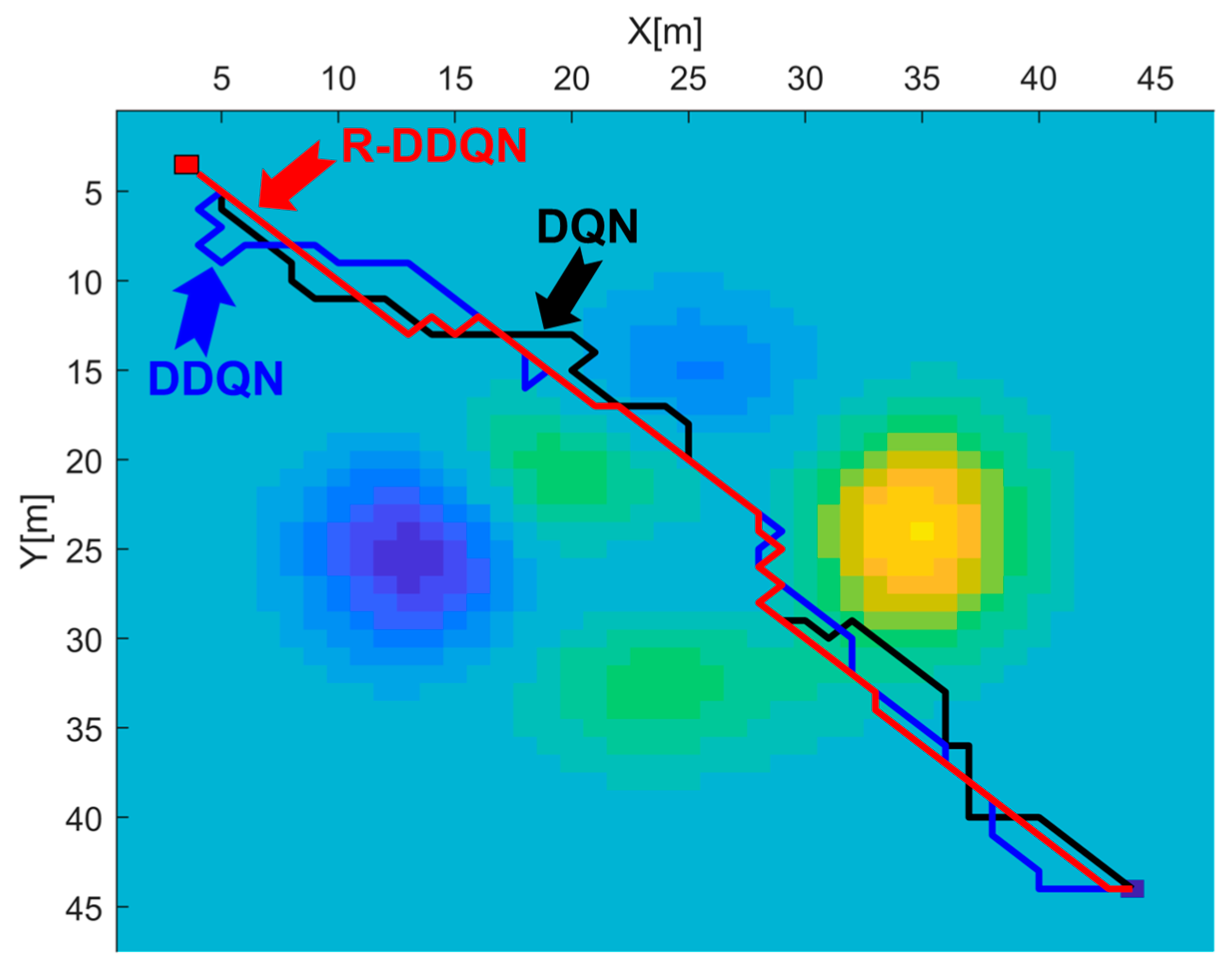
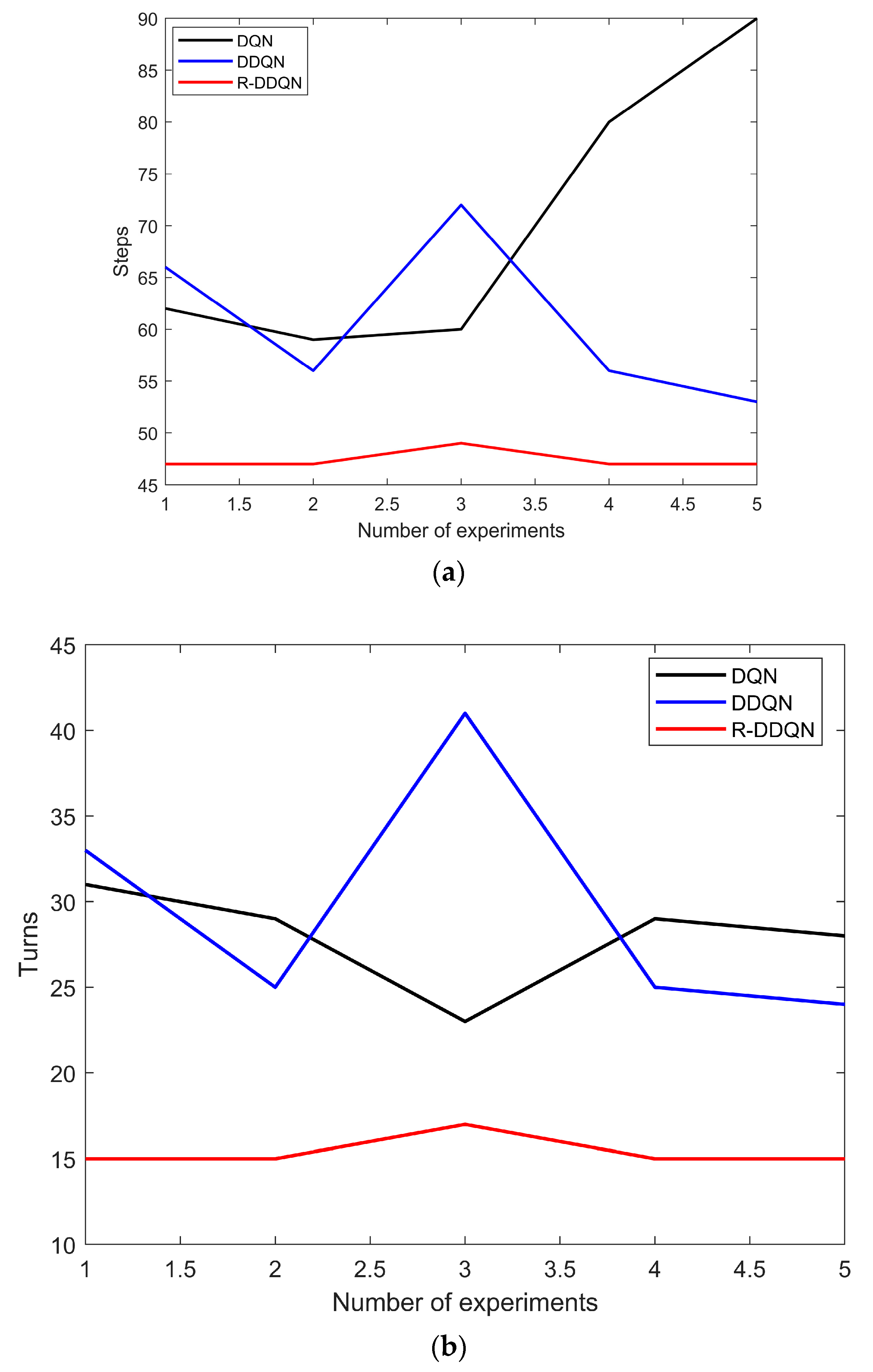
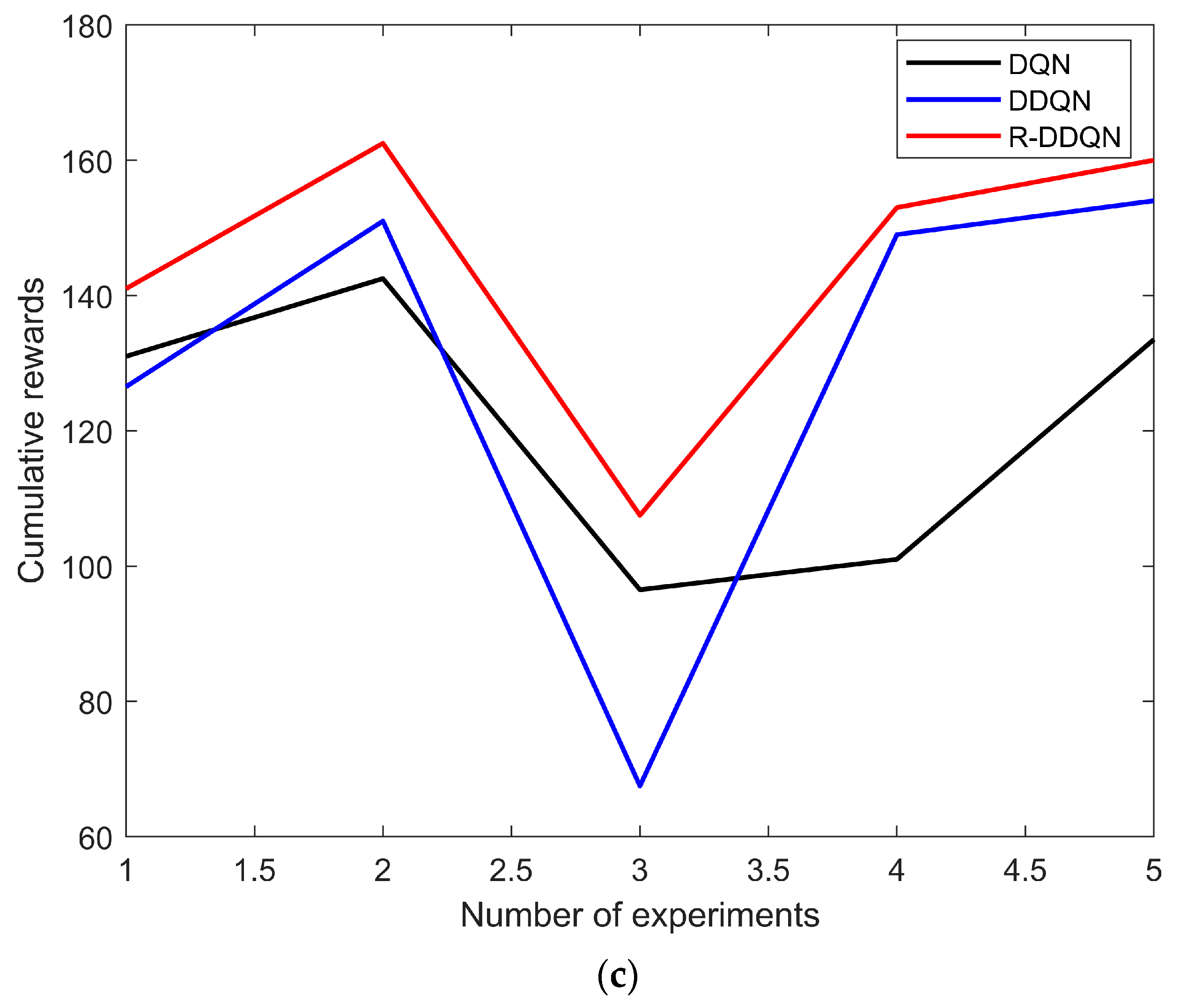
This study aims to propose a novel method for decoupling the path-evaluation and -planning algorithms through deep reinforcement learning algorithms. Our proposed method includes a 3D terrain-processing technique and an enhanced deep Q-learning method. Furthermore, we compared our approach with two other deep reinforcement learning methods. The experimental results indicate that the R-DDQL method exhibits superior performance compared to the other two methods. Specifically, the R-DDQL algorithm converges faster and achieves higher rewards in a shorter period. Moreover, the paths generated by R-DDQL are shorter and flatter than those produced by the other two methods. Finally, the generalization ability and real-time performance of the proposed method were evaluated in both static and dynamic planning tasks.

The improved performance of R-DDQL can be attributed to its retrospective mechanism, which enables it to identify and avoid the previously encountered overestimation problems during the learning process. The retrospective mechanism reduces overestimation errors during Q-value estimation, which is a common challenge faced by Q-learning-based algorithms. As a result, R-DDQL can more accurately assess the best action to be taken, resulting in a more efficient and effective path-planning strategy.

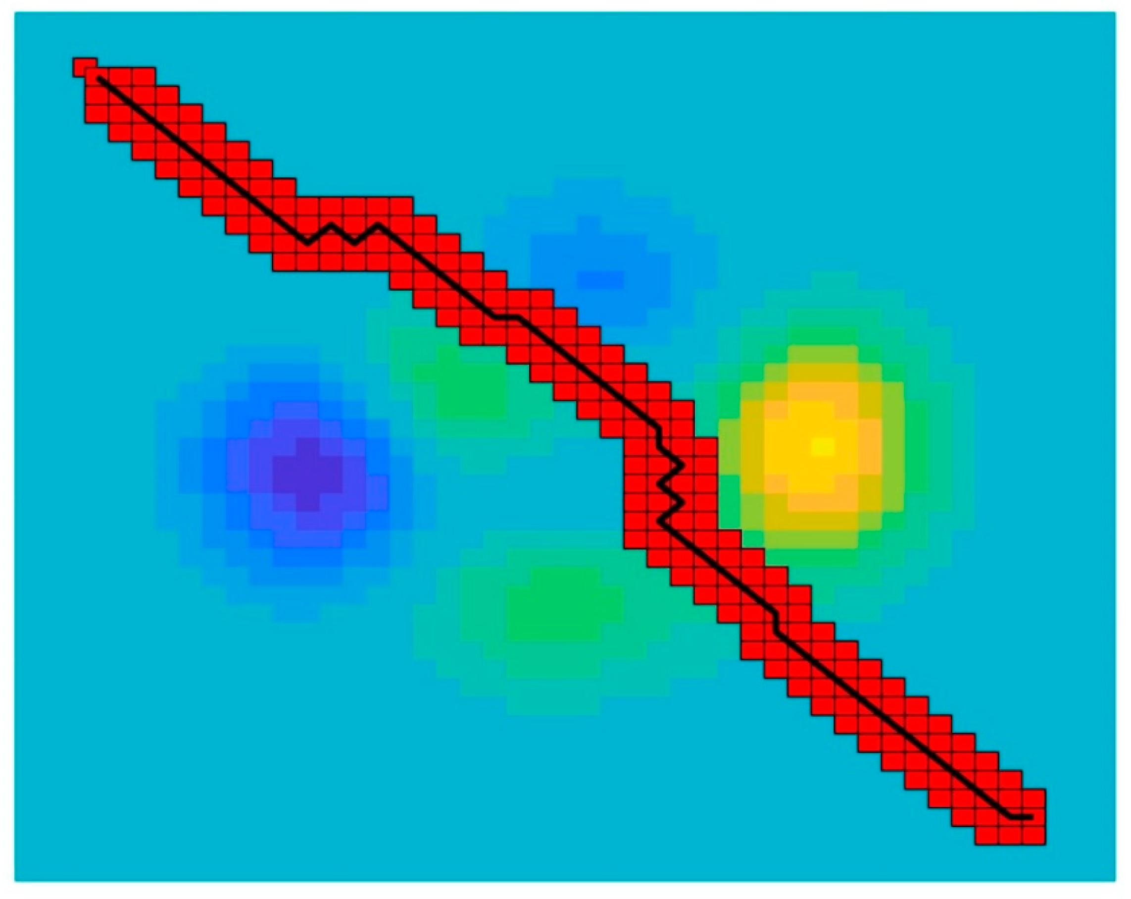
Specifically, the improvement of R-DDQL can be attributed to two factors. First, R-DDQL optimizes the samples in the memory to increase the validity of samples and reduce the proportion of invalid samples. This ensures that the training process is based on high-quality samples, which improves the overall learning performance of the algorithm. Second, while DDQL employs a depth-first approach with the help of heuristic rules, R-DDQL incorporates a retrospective mechanism based on the combination of depth-first and extended breadth strategies. The retrospective mechanism filters the high-quality solutions that are most useful for expanding the training breadth, which improves the overall efficiency of the algorithm. Figure 15 illustrates the retrospective mechanism, with the red grid indicating the raster filtered by the retrospective mechanism. These high-quality solutions are sent to the memory D, which enables the algorithm to expand the training breadth and improve its performance.

Although the retrospective mechanism guides R-DDQL, the path generated by R-DDQL is entirely different from the guidance mechanism. This implies that the retrospective mechanism can effectively guide DQL and improve its convergence speed and stability. The limitation of this method is that an algorithm needs to be developed to help DDQL improve its performance in the training phase, which will take more effort in the training phase. In future research, better retrospective mechanisms (not limited to the methods in this article) can be developed to enhance the performance of DQL.

6. Conclusions

In this study, a novel approach was proposed to improving the performance of self-learning algorithms by incorporating timely retrospection. The proposed retrospective mechanism is introduced to the DDQL algorithm to enhance its learning efficiency. This mechanism enables the algorithm to filter high-quality solutions, thereby improving the overall performance of the algorithm, resulting in a more efficient and effective path-planning strategy.

In order to be able to integrate the path costs into the map and to be able to input the R-DDQL algorithm as a whole for path planning in 3D surface terrain, we propose a 3D terrain-processing technique that uses a digital elevation model to represent the integrated costs of paths and uses functions to simulate this 3D terrain for planning. This approach is able to separate the path cost from the planning algorithm and facilitate the robot to plan according to different path-evaluation methods.

The experimental results show that R-DDQL exhibits a superior performance compared to two other deep reinforcement learning methods. Specifically, R-DDQL achieves higher rewards in a shorter period and generates shorter and flatter paths. The proposed method’s generalization ability and real-time performance were evaluated in both static and dynamic planning tasks, demonstrating its effectiveness in a wide range of scenarios.

The proposed method has been demonstrated for pathfinding in 3D terrain, but future work should focus on bridging the reality gap. The reality gap poses a challenge in obtaining a reliable training set in real-world scenarios with many uncertain factors. For DQL, a large number of episodes is necessary to obtain stable policies, which increases the risk of collision and equipment damage. Hence, further studies are required to determine how to make UGVs distinguish and avoid pedestrians in real-time and how to develop a reliable terrain-information-acquisition module that can communicate with UGV.