The Effect of Blue Noise on the Optimization Ability of Hopfield Neural Network

Abstract

Noise is ubiquitous in the real-world environment. At present, most scholars only include the stage of Gaussian white noise when applying noise in neural networks and regard white noise as a tool to optimize the network model, which is far from enough, because noise not only affects the optimization ability of the Hopfield neural network but can also better fit the needs of the actual use of the scene. Therefore, according to the problems in the existing research, a method is proposed to combine the neural network with colored noise according to the signal-to-noise ratio. Taking blue noise as an example, the anti-interference ability of the Hopfield neural network regarding colored noise is studied. The results show that for the Hopfield neural network driven by blue noise, by adjusting the neural network step size, excitation function and signal-to-noise ratio, it not only provides ideas for adding colored noise to the neural network but also enables the neural network model to have better optimization-seeking ability. The research results have some reference significance for improving the practical application of neural networks in noisy environments.

1. Introduction

In today’s ubiquitous artificial intelligence, various types of neural networks are being used more and more widely in various industries. If the interference of noise on a neural network is not considered, it is possible that no matter how perfect the performance of the network model is in training, when it is put into use, the model will always be disturbed by different levels of noise due to the difference in the usage environment and will thus face the “failure” situation caused by excessive noise influence in certain situations [1,2].

Hopfield is a feedback neural network model (HNN, Hopfield neural network), which is mainly used to solve various optimization problems [3,4] and also has a wide range of uses in real-world applications, such as image processing [5,6,7], predictive classification [8,9,10], and communication [11,12], and Hopfield neural networks are prone to generating random noise due to their physical properties. Based on this common phenomenon in real-world applications, the paper introduces blue noise into Hopfield neural networks to simulate the noise in real-world applications. Simulation experiments show that it is feasible to incorporate colored noise into a neural network, and by controlling the signal-to-noise ratio and noise spectrum, the researcher can use any real-world usage environment as a background to optimize the neural network and allow the neural network model to achieve more desirable results. Additionally, the construction of the colored noise generator tests how much interference immunity Hopfield neural networks can have in specific real-world applications without distortion, providing a theoretical basis for practical applications.

Chaotic neural networks are regarded as intelligent information processing systems which are able to realize real-world computation because of their highly nonlinear dynamic systems and close relationship with chaos. Therefore, this paper takes chaotic neural networks as the entry point. On the one hand, the feasibility of noise fusion can be verified; on the other hand, disturbance can be generated by noise to enhance the chaos of the chaotic neural network and improve the optimization rate.

The contributions of this study include demonstrating the technical feasibility of using noise fusion in conjunction with neural networks, as well as highlighting the potential applications of this approach in training neural networks and other models. This study also examines several specific neural network models that are subject to specific noise disturbances and used in optimization problems. The findings of this study may lead to the development of more effective and personalized neural network training plans, ultimately improving both the training set and algorithm accuracy.

2. Related Works

Noise exists widely in every part of nature, and in practical data processing, Gaussian white noise is generally used to approximate the stochastic rise and fall of a system, while white noise is only an ideal situation, as judged by the definition and statistical properties of white noise. Since the assumptions are based solely on Gaussian white noise, the effect of actual colored noise is not considered. As a consequence, there is a risk that data processing theories and methods may not be sufficient to guarantee the reliability of the estimation results [13]; therefore, many researchers are committed to eliminating the influence of noise [14,15]. However, it is difficult to eliminate the influence of colored noise due to the complex and changeable condition of noise. Therefore, in practical models, people use colored noise to accurately describe the behavioral system of objects [16,17,18]. For example, Nelson et al. [19] investigated adaptive grayscale compressive spectral imaging using optimal blue noise coding patterns. The importance of noise color in simulations of evolutionary systems was demonstrated by Matt et al. [20]. Zhang [21] discussed wavelet analysis of red noise and its application in climate diagnosis. Hatayama et al. [22] analyzed the effect of pink noise on EEG and memory performance in memory tasks. Liao et al. [23] studied the phase-locking of ultra-low power consumption stochastic magnetic bits induced by colored noise. Although much work has been carried out by researchers on colored noise, there is a slight lack of research regarding adding colored noise to neural networks in order to achieve a close fit to real-world usage cases.

Caglar et al. [24] introduced a novel approach that involves adding noise to the activation function of neural networks. It has been found that replacing this saturated activation function with noisy variants helps optimization in many cases, producing the most advanced or competitive results in different datasets and tasks, especially when training seems to be the most difficult. Shao et al. [25] investigated an intelligent fault diagnosis method based on a multi-scale deep convolutional neural network (MSD-CNN) model and strong noise data enhancement. Through the data enhancement method for strong noise, the number and diversity of training samples of the MSD-CNN model are improved, so that the model is able to learn deeper features in the training stage. Yang et al. [26] proposed an automated vision-based method for the surface condition recognition of concrete structures. An improved Dempster–Shafer (DS) algorithm was designed for decision-level image fusion. The robustness of the proposed method was verified by using images contaminated by various types and intensifies of noise.

After years of development, the solution rate of the neural network has reached a satisfactory effect on the optimization of the problem [27,28,29]. However, for the complex and changeable noise situation in the real environment, if the noise interference situation in the specific environment is not considered, the solution rate may be biased when the model is applied to the actual situation, so adding noise to neural network training is indeed necessary.

3. Materials and Methods

In this section, the generation process of colored noise and the model of noise fusion with the neural network will be explained. Firstly, various typical colored noises and their generation methods are introduced. Then, the fusion method of the noise and neural network is described in detail. Finally, an improved method of the network model is proposed.

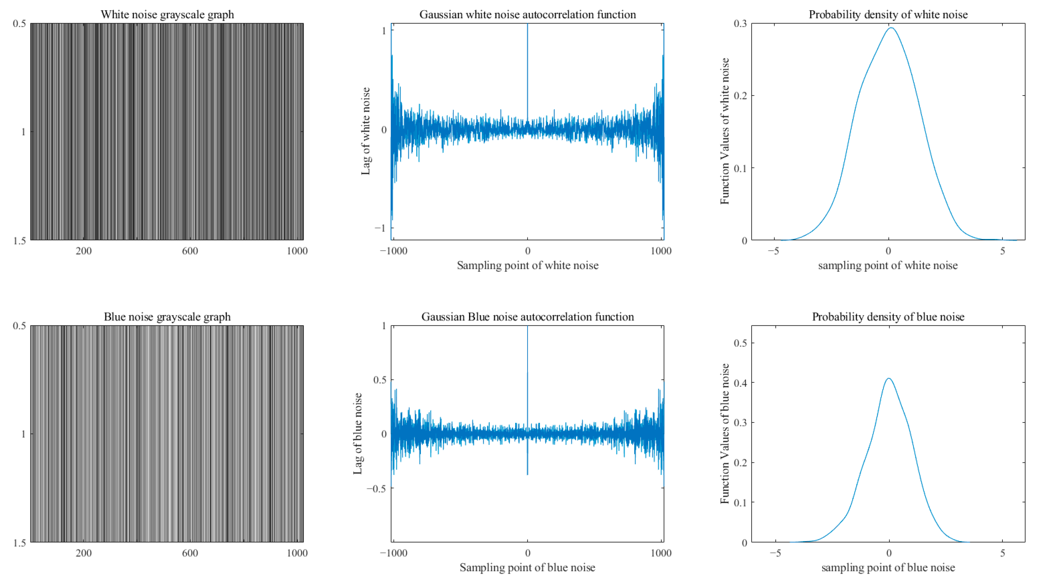
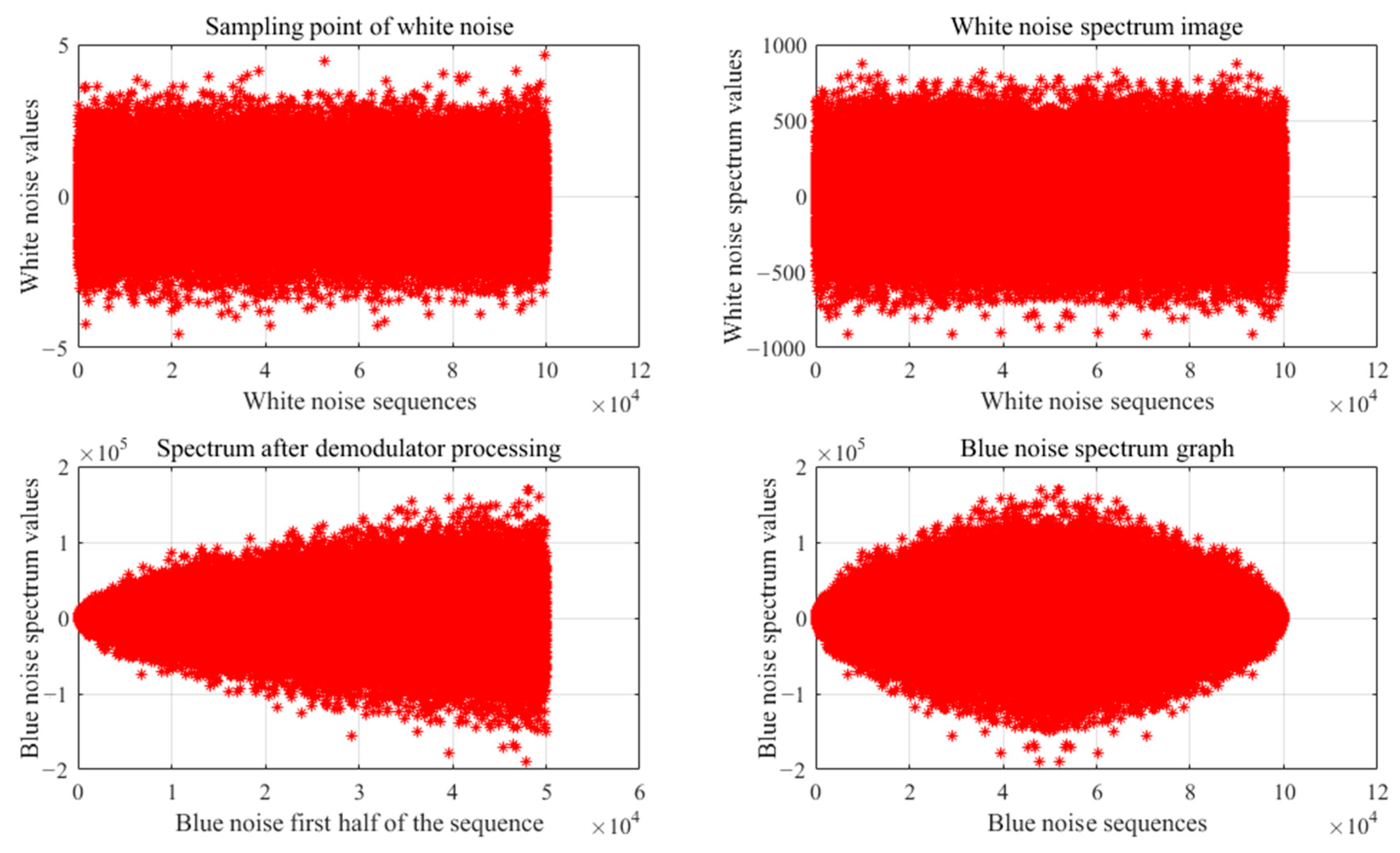
3.1. Constructing Colored Noise Generators

Noise signals are signals generated by random processes and can be generally classified as white noise and colored noise. White noise is a noise signal whose power spectral density (PSD, power spectral density) is constant in the whole frequency domain and has been widely used in the noise correlation test of various models; however, white noise as a purely theoretical construct will inevitably have deviations when simulating realistic application scenarios [30], so taking various types of spectral situations of colored noise becomes relevant. Some of the typical colored noise signals are shown in

Table 1. Example of typical colored noise.

Noise Type	PSD	Examples of Applications
Red noise	$\propto \frac{1}{f^2}$	Identifying steady-state transitions in the integrated analysis of climate records
Pink noise	$\propto \frac{1}{f}$	Promotes neural oscillatory activity
Blue noise	$\propto f$	Multi-class blue noise sampling
Violet noise	$\propto f^2$	Acoustic thermal noise signal of water

.

There are many colored noise generation methods, but in the face of the complex N-dimensional vector situation of neural networks, most of them cannot be directly applied to neural networks, so the article improves the typical $PSD\propto f^{\alpha }$ (α∈R) colored noise sequence generator [31] based on these typical colored noise types, the original noise generator can only generate colored noise sequences satisfying the one-dimensional case. After the improvement, colored noise networks matching the ranks of neural networks will be generated when the size of the ranks of neural networks is obtained and will meet the requirements of Gaussian noise distribution, based on the fusion scheme proposed in the paper, and the colored noise network will directly perturb the neural network and generate the output. Since the improved noise generator can freely choose the colored noise network dimension according to the rank value size of the neural network, the noise generator also supports the output of N-dimensional noise sequences with a single point, which is convenient for the subsequent fusion work with the neural network. Based on the original generator [32], the dimension reconstruction function is added to this generator, which is composed of fast Fourier transform (FFT), inverse fast Fourier transform (IFFT), divisor, and multipliers. The digital input signal is input continuously point by point, and the FFT transform is made first, and according to the desired colored noise, the frequency characteristic H(n) is divided in the frequency domain; then, the IFFT transform is made, and the output is reconstructed according to the desired dimension, the output of the colored noise generator is obtained cumulatively, and the colored noise after reconstruction still obeys the Gaussian distribution, so it does not cause the probability density to change, and its difference is mainly reflected in the sequence power spectral density. The difference is mainly reflected in the sequence power spectral density and its own numerical distribution. Taking blue noise as an example, the constructed noise sequence of its own characteristics and white noise is shown in Figure 1, the generated blue noise still meets the requirements of Gaussian noise distribution. However, it can be obviously seen in the gray figure that the gray value of the blue noise after spectrum transformation is higher than that of the original white noise, while the autocorrelation function and power spectral density are a Fourier transform pair, and it can be seen that the noise amplitude after re-construction is significantly reduced.

The specific construction process is as follows:

Let the Fourier transform of the white noise energy signal s(t) be S(f), then the power spectral density is as follows:

$$P(f)=\underset{T\to \infty }{\lim }\frac{1}{T}|S(f{)|}^2,$$

(1)

Taking blue noise as an example, the spectral density after the divider is as follows:

$$P(f)=\underset{T\to \infty }{\lim }\frac{1}{T}|\frac{S(f)}{\raisebox{1ex}{$1$}\!\left/ \!\raisebox{-1ex}{$\sqrt{n}$}\right.}{|}^2(n=1,2,3\dots \dots ),$$

(2)

where n ∈ N+:

$$P(f)=\underset{T\to \infty }{\lim }\frac{n}{T}|S(f){|}^2(n=1,2,3\dots \dots ),$$

(3)

where n is the frequency index, and instead of the true frequency f, S(f) is constant in the whole frequency domain; thus, it is easy to see that the blue noise power spectral density P(f) is proportional to f. Since the spectral density is generally symmetric, the complete spectrum amplitude of blue noise is obtained via conjugate flip copy after the half spectrum is processed by the divisor. Other types of noise can be constructed by referring to the spectrum information presented in Table 1 and Formula (2). The spectrum change process is shown in Figure 2. The two pictures in the upper half are the noise and spectrum distribution under white noise, while the two pictures in the lower half are the spectrum distribution after the divisor processing and the complete blue noise spectrum distribution after the conjugate flip copy.

After obtaining the N-dimensional colored noise sequence, the colored noise and the original neural network sequence can be fused. Since the noise sequence has been processed, it has now become a pattern of N-dimensional vectors, which is mathematically described as follows: if the input data sequence is {A}, the observation sequence L1, L2,…, Lt has the observation equation at moment t:

$$Lt=AtXt+et,$$

(4)

$$et=k\times Gt,$$

(5)

where Xt is the parameter vector at moment t; At is the column full rank design matrix; et is the true error vector; Gt is the Gaussian colored noise sequence; and k is the required noise ratio for the actual environment. Where k determines the value according to the required Signal Noise Ratio (SNR), and according to the SNR calculation formula [33], the derivation process is as follows:

$$SNR=10\lg (\frac{P_{At}}{P_{et}}),$$

(6)

It is clear that:

$$p_{et}={10}^{(\lg P_{At}-\frac{SNR}{10})},$$

(7)

or written as:

$$P_{et}=\frac{p_{At}}{{10}^{\frac{SNR}{10}}},$$

(8)

where SNR is the signal-to-noise ratio of the sequence At to et at moment t, P_At is the power of the sequence At and P_et is the power of the sequence et. The power density of the noise signal P_et can be measured according to the power density formula:

$$p_{et}=\frac{{\displaystyle \sum _{i=0}^m{\displaystyle \sum _{j=0}^n{(k\times x_{ij})}^2}}}{N}=k^2\times \frac{{\displaystyle \sum _{i=0}^m{\displaystyle \sum _{j=0}^n{(x_{ij})}^2}}}{N}=k^2\times p_{Gt},$$

(9)

where: m and n represent the number of rows and columns of the matrix, N represents the number of matrix elements, P_Gt is the Gaussian colored noise power density, as the mean value of the constructed colored noise is 0 and the variance is 1, so it is easy to know that the P_Gt power density is 1 through the variance Formula (10).

$$S^2=\frac{{\displaystyle \sum _{i=1}^n{(x_i-\overline{x})}^2}}{N}(where \overline{x}\mathrm{is}\mathrm{the}\mathrm{matrix}\mathrm{mean}),$$

(10)

From Equations (9) and (10) it is easy to see that:

$$p_{et}=k^2\times p_{Gt}=k^2,$$

(11)

The conjunction of Equations (8) and (11) yields:

$$p_{et}=k^2=\frac{p_{At}}{{10}^{\frac{SNR}{10}}},$$

(12)

It is clear that:

$$k=\sqrt{\frac{p_{At}}{{10}^{\frac{SNR}{10}}}},$$

(13)

In this paper, the reason why SNR is used as the basis for the fusion of neural network and colored noise in this paper is that this method is undoubtedly the most friendly and helpful to understand for researchers who want to study noise. Blue noise is chosen as the sample of article fusion because blue noise, as a typical noise, is undoubtedly representative. Subsequent researchers can simulate the real noise environment by means of probability sampling [34] and attribute noise monitoring [35].

3.2. Blue Noise Hopfield Neural Network Model

Construct the Hopfield neural network model with blue noise as:

$$U_c=Cn(U),$$

(14)

$$V=\frac{1}{2}(1+\tanh (\frac{U_c}{{\epsilon }_0})),$$

(15)

$$V_c=Cn(V),$$

(16)

$$Cn(\xi )=ABGN(\xi ,SNR,m,n),$$

(17)

U and V in this network model are the input and output of the Hopfield network [36], U_c and V_c are the input and output perturbed by colored noise, ${\epsilon }_0$ is the steepness parameter of the excitation function, and ABGN is the blue noise combined with the original signal function, where m and n are the row and column values of the input and output matrix. The output V of the Hopfield network is generated using a nonlinear function. In this network model, the input and output of the neural network are contaminated by colored noise, the purpose of which is to study the anti-interference ability of colored noise in the Hopfield neural network.

3.3. Improvement of Neural Network Model Based on Colored Noise

Through the above experiments, this paper proves that colored noise can improve the optimization of the neural network. To verify that the colored noise neural network model can meet the needs of more scenarios, the original Hopfield neural network model is improved, and the excitation function of the original neural network model is transformed from Sigmoid function to a combination of continuous wavelet and Sigmoid excitation function. The chaos generation mechanism of the improved neural network is also introduced through the exponential decreasing of the self-feedback terms. Since the excitation function of the wavelet chaotic neural network does not monotonically increase but generally increases, the addition of wavelet function can not only cause the excitation function non-monotonically to increase but also to allow the excitation function to have wavelet function advantages. The improved model is applied to the traveling salesman problem in 30 cities through the segmented simulated annealing mechanism and the disturbance of blue noise. Comparing the data from previous experiments, it can be intuitively felt that the network model, adding the wavelet function and the segmented simulated annealing mechanism, has significantly improved the solving rate. Even in the face of more complex combinatorial optimization problems, colored noise perturbation can still improve the solution of chaotic neural networks.

The improved Hopfield neural network model is as follows:

$$U_c=Cn(U),$$

(18)

$$V=S(U_c,{\epsilon }_0)+coef\cdot M(U_c,{\epsilon }_1),$$

(19)

$$V_c=Cn(V),$$

(20)

$$Cn(\xi )=ABGN(\xi ,SNR,m,n),$$

(21)

$$S(U_c,{\epsilon }_0)=\frac{1}{1+e^{-U_c/{\epsilon }_0}},$$

(22)

$$M(U_c,{\epsilon }_1)=\frac{2}{\sqrt{3\sqrt{\pi }}}(1-{(\frac{U_c}{{\epsilon }_1})}^2)\exp (-\frac{{(U_c/{\epsilon }_1)}^2}{2}),$$

(23)

Equation (19) is the excitation function of wavelet chaotic neural network, which is composed of Sigmoid function and Mexican_Hat function. Where S represents Sigmoid function and M represents Mexican_Hat function; ${\epsilon }_0$ and ${\epsilon }_1$ are steepness parameters of Sigmoid function and Mexican_Hat wavelet function; coef is a coefficient (coef $\ge$ 0); and other parameters have the same meaning as the parameters of Hopfield neural network model chaos with blue noise.

4. Results and Discussion

4.1. Blue Noise Hopfield Neural Networks in Optimization Problems

Optimization problems are divided into two kinds of function optimization and combinatorial optimization. Many practical problems can be categorized into one of these for solving [37,38]. To verify the immunity of Hopfield neural network to colored noise, blue noise was selected to perturb the input and output, respectively, and the effect of noise on Hopfield function optimization and combinatorial optimization problems was explored.

The essence of solving optimization problems with Hopfield is in the process of solving the extremum of the energy function E of that neural network, so the constraints of the problem need to be expressed in the form of a function of that energy.

The algorithm flow is as follows:

(1)

The problem to be solved is described in computer language, where the output of the neural network corresponds to the solution of the problem.

(2)

Construct the energy function of the neural network so that its minimum value corresponds to the optimal solution of the problem.

(3)

The initial states of the neurons are generated, and the weights W and bias inputs I between the neurons are corrected via the output values of each iteration after noise perturbation.

(4)

In the case that the energy function has converged, and the output accuracy is satisfied, the steady state of its operation is the optimal solution under certain conditions.

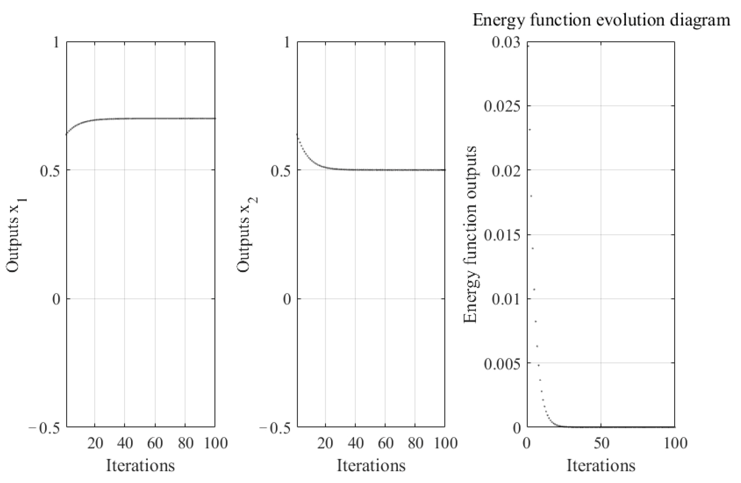
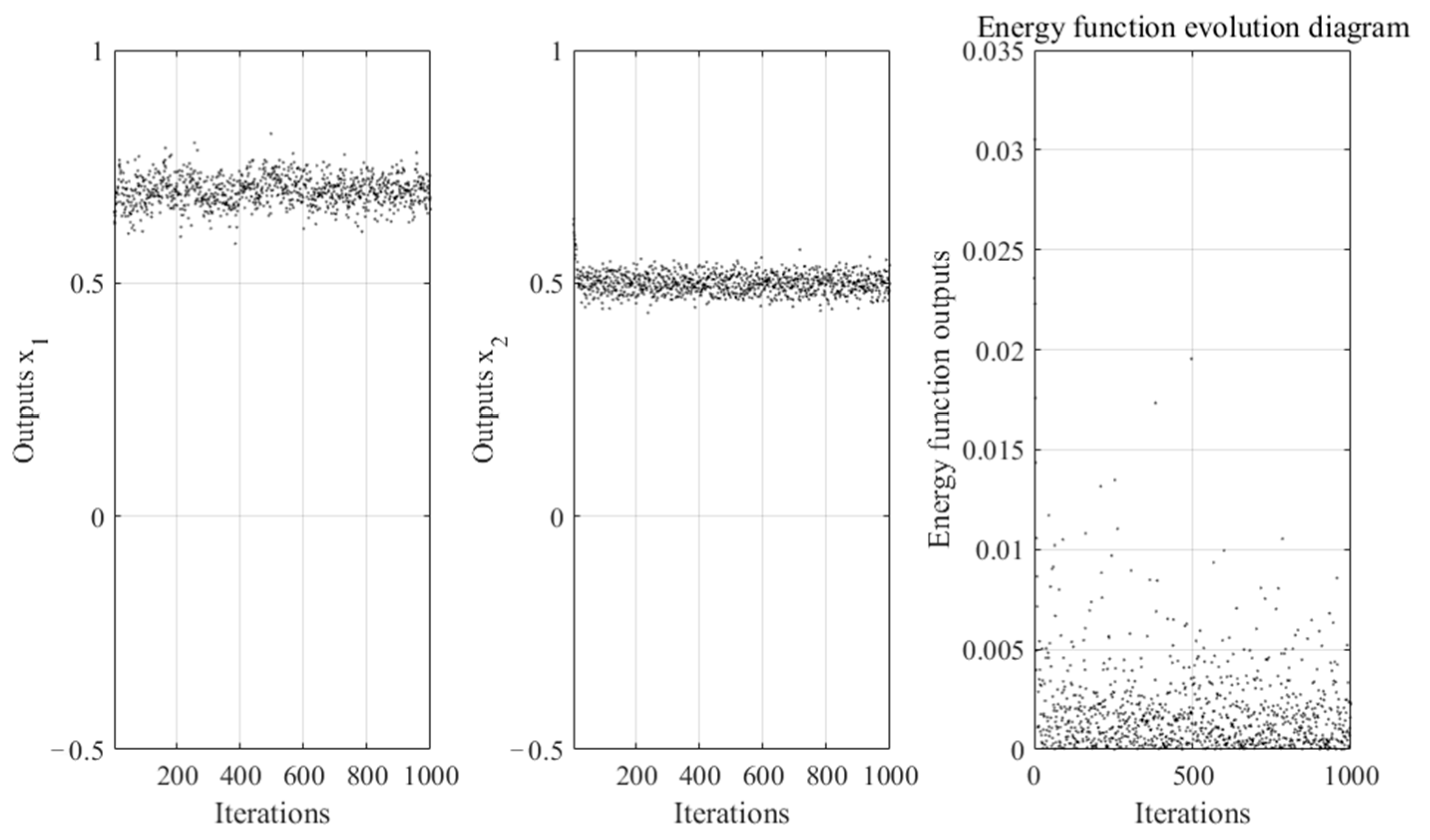
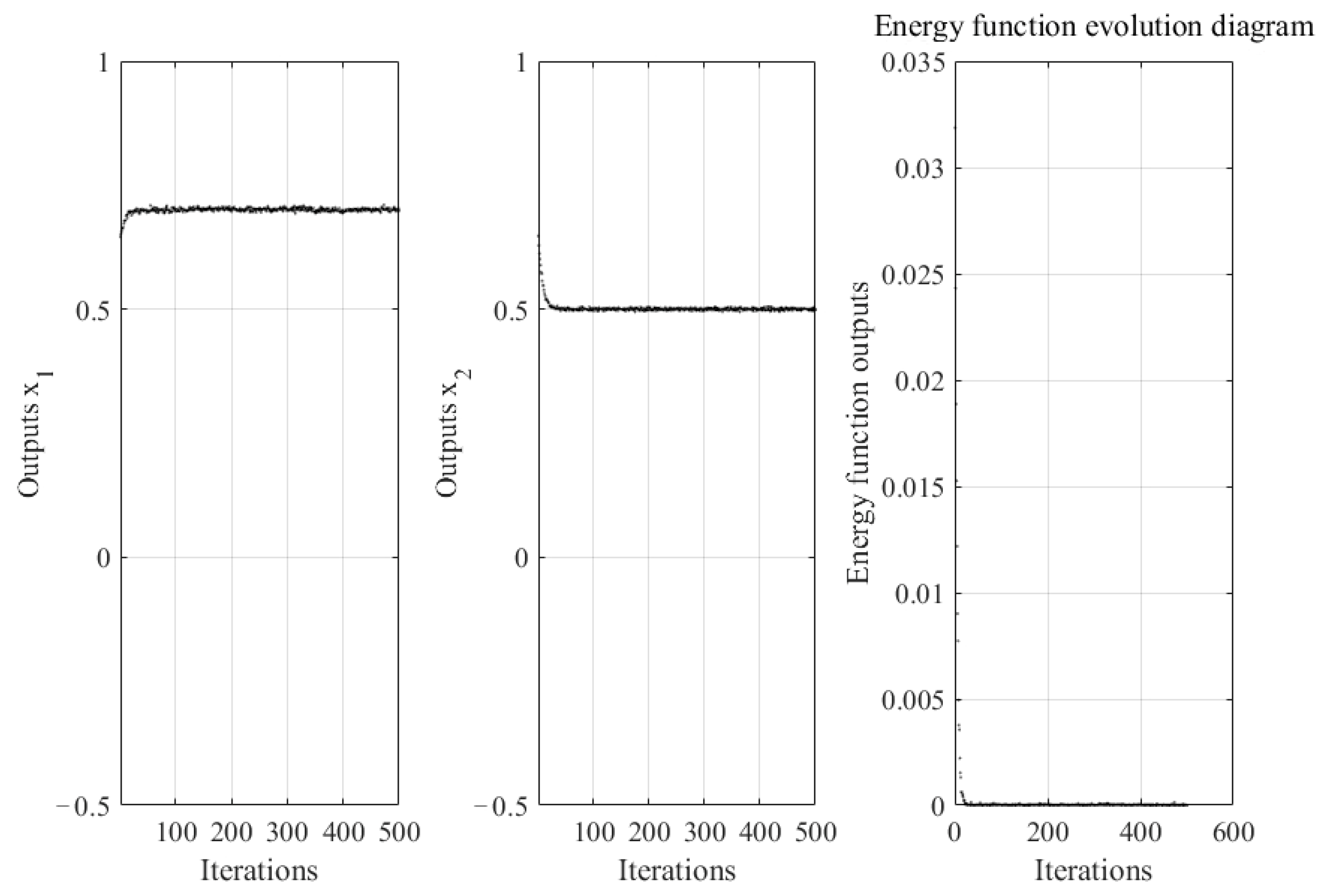
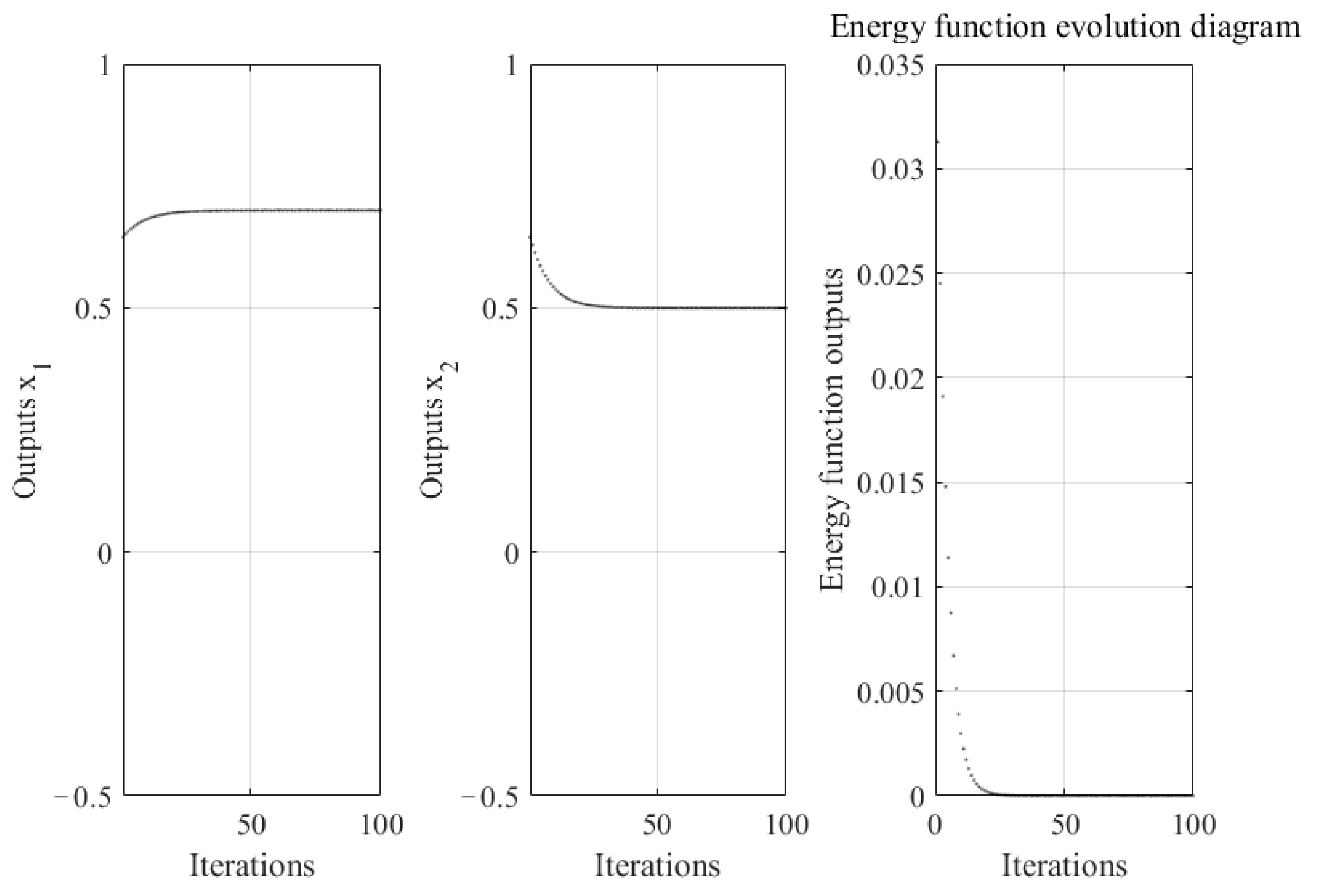
4.1.1. The Effect of Blue Noise on the Ability of Neural Networks to Optimize Continuous Functions

The statistical analysis of the Hopfield neural network’s ability to optimize Equation (24) [39,40] under blue noise perturbations with different signal-to-noise ratios.

$$f(x_1,x_2)={(x_1-0.7)}^2[{(x_2+0.6)}^2+0.1]+{(x_2-0.5)}^2[{(x_1+0.4)}^2+0.15],$$

(24)

It is easy to see that the function has a minimum value of 0, corresponding to the coordinates (0.7, 0.5), and is the global minimum of the objective function. There are three of these local minima, namely (0.6, 0.4), (0.6, 0.5), and (0.7, 0.4).

The function is solved using the network model in this paper with the set parameters: step t = 0.1 and excitation function coefficient = 0.5. The evolution of the energy function of the Hopfield neural network solution function with x₁, x₂ under a different signal-to-noise ratio of blue noise perturbation is shown in Figure 3, Figure 4, Figure 5 and Figure 6.

Figure 3 shows the noise-free scenario, and the solution process of the neural network is as follows: the network reaches an unstable state after the search, at which time the network starts gradient descent and soon reaches a stable state, searching for the global minimum point (0.7, 0.5) with a minimum value of 0.

It can be seen from Figure 4 that when the SNR is 30, it has a great impact on the neural network and never reaches a stable state, and after 1000 iterations, the global minimum point (0.6917, 0.5043) is searched for at this time, with a minimum value of 1.1537 × 10⁻⁴ and a minimum value of 1.12 × 10⁻² in the literature [41].

Figure 5 shows the solution of the neural network when the SNR is 50. Although after 500 iterations, a stable state is still not reached, the floating range is very close to the correct solution, and at this point, the global minimum point (0.7014, 0.5002) is searched for, with a minimum value of 2.5668 × 10⁻⁶ and the minimum value of 5.3560 × 10⁻⁶ in the literature [41].

It can be seen from Figure 6 that when the SNR is 90, the interference of noise for the neural network is basically negligible and achieves the same effect as when there is no noise, when the global minimum point (0.7000, 0.5000) is searched for with a minimum value of 6.0226 × 10⁻¹⁰ and a minimum value of 6.2693 × 10⁻¹⁰ in the literature [41].

From the above experiments, it can be seen that the presence of noise has an impact on the optimization ability of Hopfield neural network; in particular, when the signal-to-noise ratio is less than 50, the convergence speed of the energy function is greatly affected, and the impact on the solution ability is also great, but when the signal-to-noise ratio is greater than 90, the noise has little effect on the network model, and the optimization performance of this network model reaches the same degree as the ideal noise-free environment. The comparison with the optimization results conducted in the literature [41] also shows the superiority of this model, and the range of the anti-interference ability of the Hopfield neural network under the influence of blue noise is sought.

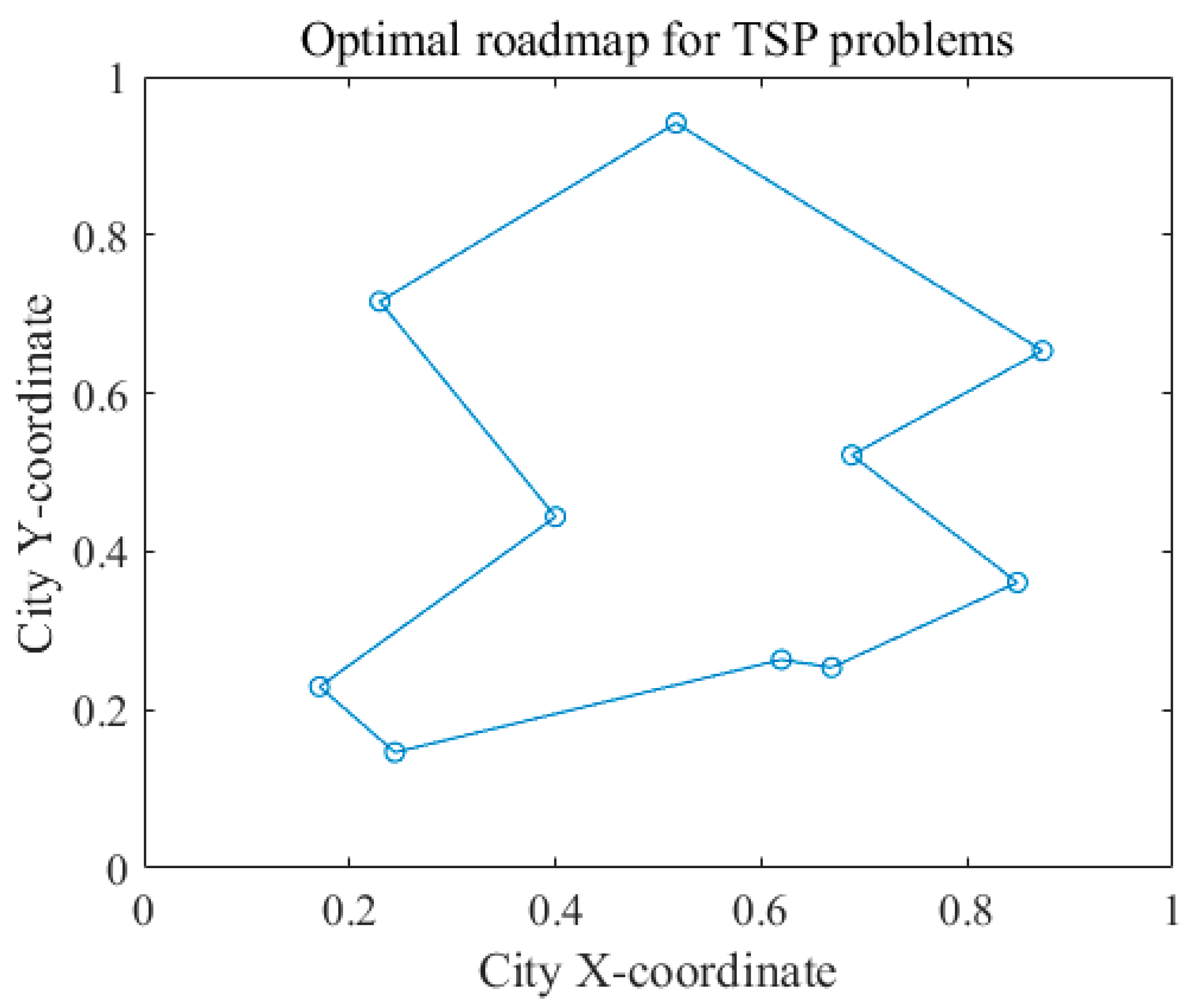
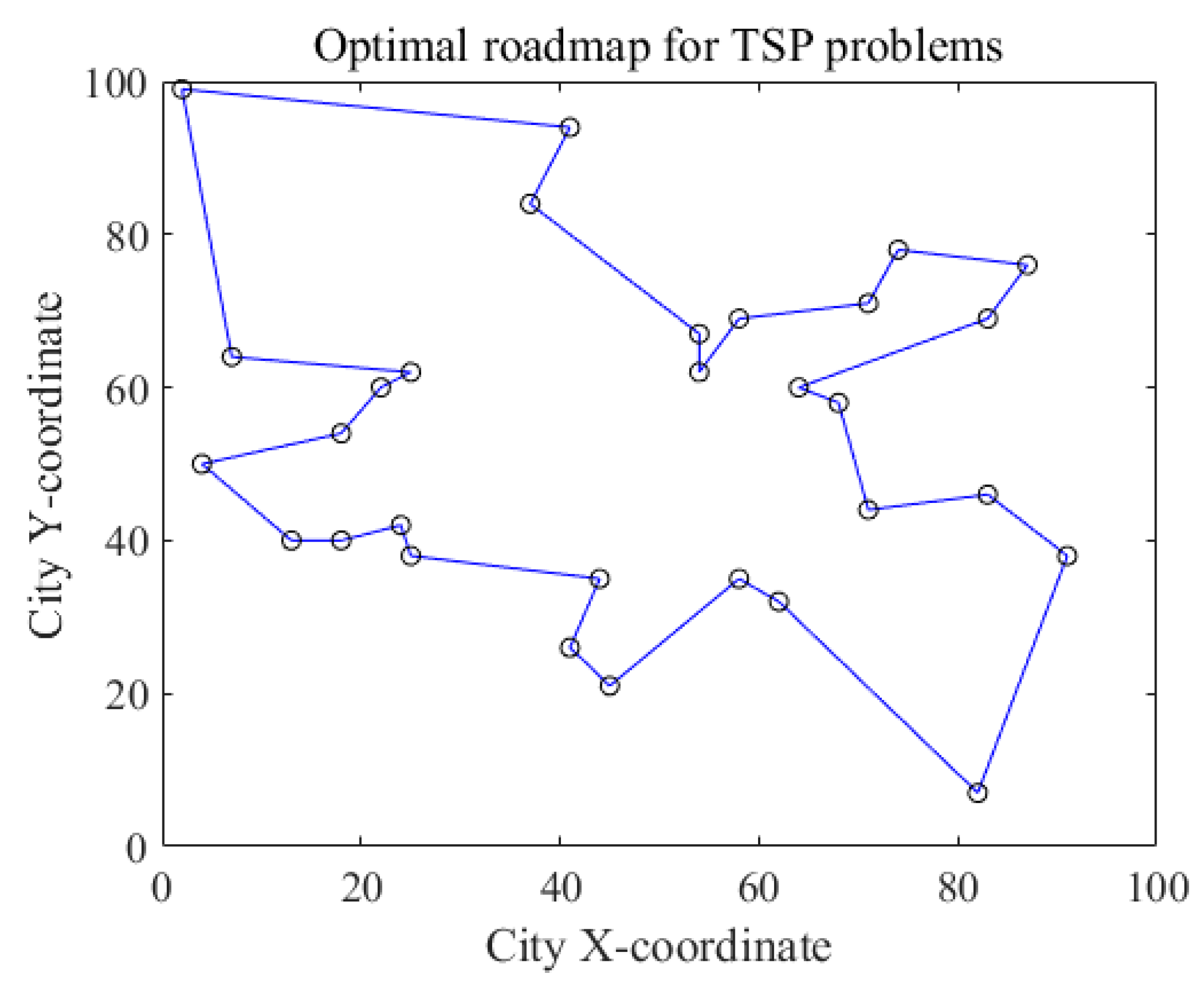
4.1.2. The Effect of Blue Noise on the Optimization Power of Neural Networks for Combinatorial Problems

In this paper, the colored noise Hopfield neural network is applied to the 10-city traveling salesman problem (TSP) [42,43,44]. The traveling salesman problem is described as the shortest loop required to visit each city once and return to the starting city, given the distance between two cities.

The energy function to take the shortest path and satisfy all constraints [45,46] is shown in Equation (25). Where V_xi denotes that the xth city is visited on the ith order and d_xy is the distance between cities x and y. Therefore, the global minimum E value reached after several iterations represents the shortest effective path.

$$E=\frac{A}{2}{\displaystyle \sum _{x=1}^n({\displaystyle \sum _{i=1}^n{V}_{xi}-1{)}^2+\frac{B}{2}}}{\displaystyle \sum _{i=1}^n({\displaystyle \sum _{x=1}^n{V}_{xi}-1{)}^2+\frac{D}{2}}}{\displaystyle \sum _{x=1}^n{\displaystyle \sum _{y=1}^n{\displaystyle \sum _{i=1}^n{d}_{xy}{V}_{xi}{V}_{y,i+1}}}}$$

(25)

In this paper, we use 10 cities after classical normalization, with the following coordinates: (0.4, 0.4439); (0.2439, 0.1463); (0.1707, 0.2293); (0.2293, 0.716); (0.5171, 0.9414); (0.8732, 0.6536); (0.6878, 0.5219); (0.8488, 0.3609); (0.6683, 0.2536); and (0.6195, 0.2634). The shortest path for these 10 cities is 2.6776, as shown in Figure 7.

When solving the TSP problem with the Hopfield neural network model with blue noise perturbation, the parameters were initialized as [47]: A = B = 1, D = 1, ${\epsilon }_0$ = 0.02, and randomly generated U. The solution was performed in simulation experiments using different signal-to-noise ratios, and the experimental results were compared and analyzed.

Table 2. Experimental simulation results for different values of the parameter SNR.

	SNR	Legal Path	Optimal Path	Legal Ratio	Optimal Ratio
	Noiseless	163	118	81.5%	59.0%
This paper	40	40	7	20.0%	3.5%
Reference [41]		84	13	42.0%	6.5%
This paper	50	118	54	59.0%	27.0%
Reference [41]		126	64	63.0%	32.0%
This paper	60	156	111	78.0%	55.5%
Reference [41]		144	92	72.5%	47.0%
This paper	70	162	116	81.0%	58.0%
Reference [41]		145	94	80.0%	56.0%
This paper	80	163	117	81.5%	58.5%
Reference [41]		160	112	75.5%	53.0%
This paper	90	169	128	84.5%	64.0%
Reference [41]		151	106	74.5%	51.5%
This paper	120	161	109	80.5%	54.5%
Reference [41]		149	103	74.5%	51.5%
This paper	150	164	113	82.0%	55.5%
Reference [41]		149	104	74.5%	52.0%
This paper	180	166	114	83.0%	57.0%
Reference [41]		152	103	76.0%	51.5%

shows the simulation test data for 200 randomly assigned initial values when the colored noise parameter is taken to different values and compared with the simulation results from the literature [41].

As shown in Table 2, it is completely feasible to introduce noise into the neural network using the method of this paper. Moreover, the moderate introduction of noise signals does not have much impact on the solving ability of Hopfield neural network, and it can be seen through extensive testing that when the SNR is less than 50, the ability of this network model to solve the TSP problem is decreasing significantly, while when the SNR is greater than 90, the noise on the neural network’s ability to influence is basically negligible or even beneficial. When compared with the literature [41], it is found that by introducing blue noise and properly correcting the parameters, Hopfield obtains better optimization ability when the SNR is greater than 60, but due to the intrinsic characteristics of blue noise, which allow the network model to obtain better solution effects in white noise when the SNR is less than 60, it also provides a reference interval for subsequent researchers to ensure the SNR of the input signal sequence and the range in which the parameters are best controlled when using the Hopfield neural network.

4.2. Chaotic Neural Network Model Based on Blue Noise

Energy function selection is the same as before, ${\epsilon }_0=0.6$, ${\epsilon }_1=125$ remains unchanged, and coef is equal to 0 and 1/250, respectively. Let the simulation program take the 30 cities after classical normalization. Let the emulator take the classic 30 cities [48], and the coordinates are as follows: (41,94); (37,84); (54,67); (25,62); (7,64); (2,99); (68,58); (71,44); (54,62); (83,69); (64,60); (18,54); (22,60); (83,46); (91,38); (25,38); (24,42); (58,69); (71,71); (74,78); (87,76); (18,40); (13,40); (82,7); (62,32); (58,35); (45,21); (41,26); (44,35); and (4,50). The shortest path of the 30-city TSP problem is 423.7406, and its shortest path is shown in Figure 8.

When using the Hopfield neural network model with blue noise perturbation to solve the TSP problem, a self-feedback term $z_i\left(t\right)$ with a piece-wise simulated annealing mechanism is introduced, where the formula is as follows:

$$z_i(t+1)=\{\begin{array}{cc}(1-{\beta }_1)z_i(t),& z_i(t)>0.4\\ (1-{\beta }_2)z_i(t),& otherwise\end{array},$$

(26)

Let ${\beta }_1=0.01$, ${\beta }_2=0.02$, and $z_i\left(1\right)=0.1$. This enables the neural network not only to give full play to the chaotic search ability but also to maintain a reasonable convergence rate. In the simulation experiment, different SNR and excitation function coefficients coef are used, and the experimental results are compared and analyzed.

Table 3. Simulation results of the solved 30-city travel salesman problem.

coef	SNR	Legal Path	Optimal Path	Legal Ratio	Optimal Ratio
coef = 0	0	91	21	91.0%	21.0%
	30	87	12	87.0%	12.0%
	60	99	26	99.0%	26.0%
	90	93	22	93.0%	22.0%
coef = 1/250	0	100	27	100%	27.0%
	30	100	21	100%	21.0%
	60	100	31	100%	31.0%
	90	100	27	100%	27.0%

shows the simulation test data of 100 times randomly assigned initial values when different values of colored noise parameters are taken. The program simulation results are shown in the table below:

As can be seen from the above table, the improved neural network model performs perfectly when solving the legal path, which is significantly improved compared with the previous neural network model. As noise will affect network optimization within a certain range, it can be seen that when SNR = 30, the noise interference is too strong and the performance of the neural network on the optimal path is not as good as that without noise interference. However, when SNR = 60, the noise disturbance enhances the chaos of the neural network, revealing better solving performance. By transforming the original neural network model’s excitation function into a combination of the Mexican_Hat function e and Sigmoid excitation function, the solving performance of the neural network model can also be improved. When coef = 1/250, the solving ability of the excitation function is the best.

The performance index J in is used to compare various algorithms, including chaotic simulated annealing algorithms (CSA) [49] and hysteretic chaotic neural network algorithms, in the literature (HCNN) [50]. The index J can be described as:

$$J=\frac{Avg-Opt}{Opt},$$

(27)

where Avg represents the average solution and Opt represents the optimal solution. The smaller the value of index J, the better the network optimization performance. The experiment was repeated 100 times. The simulation results are shown in

Table 4. Comparison of TSP algorithms in 30 cities.

Algorithm	Optimal Solution	Index J
SCA	14	5.37%
HCNN	20	3.45%
CNNBN	31	2.53%

.

With the increase in the scale of the problem city, the performance of various algorithms decreases. Compared with other algorithms, the chaotic neural network based on blue noise has a great advantage in solving the 30-city traveling salesman problem. Because the improved neural network uses the piece-wise simulated annealing strategy, it not only fully guarantees that the neural network can carry out sufficient chaotic search but also does not excessively reduce the convergence rate. Moreover, the new excitation function is used to enhance the ergodic degree of the network chaotic rough search and enrich the dynamic characteristics of chaotic rough search. However, although the introduction of self-feedback connection causes the Hopfield neural network to display chaotic phenomena, it is often not stable, and stability is an important index for measuring the performance of a network. Although the chaotic simulated annealing strategy improves this defect and gives the network good stability, its chaotic search area is usually a local area or fragment area, and it is easy for it to fall into the local minimum point. Although the random simulated annealing strategy can be searched for in the whole state region, it is too slow. Therefore, random blue noise is introduced into the improved network model, which combines the advantages of chaotic simulated annealing strategy and random simulated annealing strategy well, and further improves the solving ability of the neural network.

4.3. Discussion

This method can effectively address the issue of fusing neural networks and colored noise. Moreover, the chaotic neural network, due to its intrinsic characteristics, exhibits better solving ability when subject to noise disturbance. The proposed method in this paper eliminates the need for extensive human and material resources to sample specific scenes. Instead, it only requires a dataset that includes the noise detected in a particular environment, thus achieving the simulation goal without incurring additional costs. However, the proposed method is currently limited to the simulation stage and can only demonstrate the effectiveness of the noise fusion method. To validate its performance in real-world scenarios, further research is needed to train and test the error rate in such environments.

Although this paper only tests the simulation on continuous function optimization and TSP problems, the proposed method can also yield excellent results for other optimization problems. Although it remains to be seen whether the data with added noise can truly replace the samples in a specific environment, it has been verified that the chaos of chaotic neural networks can be enhanced by adding noise, leading to improved solution rates.

5. Conclusions

In this paper, the color noise generation scheme with custom spectral slope is improved so that the improved generator can meet the needs of neural networks. A novel method combining colored noise and an original signal sequence according to signal-to-noise ratio is proposed, and the effect of noise on the Hopfield neural network is systematically analyzed by introducing blue noise into a simulation experiment. Moreover, the paper improves the original neural network by changing the excitation function and introducing the piece-wise simulated annealing mechanism to improve the performance of the neural network in the face of more complex combinatorial optimization problems. In the simulation results, applying the Hopfield neural network based on colored noise in function optimization and combinatorial optimization, it can be seen that the Hopfield neural network has very good robustness in noise resistance ability, and the appropriate addition of noise can also help the neural network improve optimization ability. In conclusion, this study presents a new approach to training neural networks that can actively simulate real-world noise environments. This allows models to be trained in laboratory settings to account for noise disturbances in specific scenarios, which can prevent models from performing well in the laboratory but failing in real-world applications, ultimately improving the overall accuracy of the neural network. However, to establish the reliability and effectiveness of this method, further research is needed to evaluate its performance in real-world environments and to expand its training range and application.

The research results indicate that it is possible to consider the noise conditions in specific environments during training for fusion in order to avoid a significant amount of repetitive sampling work. A training dataset can be created for models in various scenarios, provided that different noise characteristics are incorporated. Furthermore, adding noise perturbations can also be beneficial for improving the accuracy of neural networks. While the study evaluated the accuracy of the model under noise perturbations, further research is required to explore how to construct a more realistic spectral noise scenario and how to combine this approach with other neural network techniques, such as cyclic and graph neural networks. Our next research focus will be the examination of the corresponding noise perturbation of neural networks in different application fields by considering the noise characteristics specific to each scenario.

References

1. Ran, X.; Zhou, X.; Lei, M.; Tepsan, W.; Deng, W. A Novel K-Means Clustering Algorithm with a Noise Algorithm for Capturing Urban Hotspots. Appl. Sci. 2021, 11, 11202. [Google Scholar] [CrossRef]
2. Gupta, S.; Gupta, A. Dealing with noise problem in machine learning data-sets: A systematic review. Procedia Comput. Sci. 2019, 161, 466–474. [Google Scholar] [CrossRef]
3. Fung, C.H.; Wong, M.S.; Chan, P.W. Spatio-Temporal Data Fusion for Satellite Images Using Hopfield Neural Network. Remote Sens. 2019, 11, 2077. [Google Scholar] [CrossRef]
4. Rezapour, S.; Kumar, P.; Erturk, V.S.; Etemad, S. A Study on the 3D Hopfield Neural Network Model via Nonlocal Atangana–Baleanu Operators. Complexity 2022, 2022, 6784886. [Google Scholar] [CrossRef]
5. Xu, X.; Chen, S. Single Neuronal Dynamical System in Self-Feedbacked Hopfield Networks and Its Application in Image Encryption. Entropy 2021, 23, 456. [Google Scholar] [CrossRef] [PubMed]
6. Citko, W.; Sienko, W. Inpainted Image Reconstruction Using an Extended Hopfield Neural Network Based Machine Learning System. Sensors 2022, 22, 813. [Google Scholar] [CrossRef]
7. Xu, Y.Q.; Zhen, X.X.; Tang, M. Dynamical System in Chaotic Neurons with Time Delay Self-Feedback and Its Application in Color Image Encryption. Complexity 2022, 2022, 2832104. [Google Scholar] [CrossRef]
8. Xiao, Y.; Zhang, Y.; Dai, X.; Yan, D. Clustering Based on Continuous Hopfield Network. Mathematics 2022, 10, 944. [Google Scholar] [CrossRef]
9. Hillar, C.; Chan, T.; Taubman, R.; Rolnick, D. Hidden Hypergraphs, Error-Correcting Codes, and Critical Learning in Hopfield Networks. Entropy 2021, 23, 1494. [Google Scholar] [CrossRef]
10. Mohd Jamaludin, S.Z.; Mohd Kasihmuddin, M.S.; Md Ismail, A.I.; Mansor, M.A.; Md Basir, M.F. Energy Based Logic Mining Analysis with Hopfield Neural Network for Recruitment Evaluation. Entropy 2021, 23, 40. [Google Scholar] [CrossRef]
11. Yang, H.; Liu, Z. An optimization routing protocol for FANETs. EURASIP J. Wirel. Commun. Netw. 2019, 2019, 120. [Google Scholar] [CrossRef]
12. Kandali, K.; Bennis, L.; Bennis, H. A new hybrid routing protocol using a modified K-means clustering algorithm and continuous hopfield network for VANET. IEEE Access 2021, 9, 47169–47183. [Google Scholar] [CrossRef]
13. Yang, Y.X.; Cui, X.Q. Dynamic positioning colored noise influence function—A first order ar model as an example. J. Surv. Mapp. 2003, 2003, 6–10. [Google Scholar]
14. Aviles-Espinosa, R.; Dore, H.; Rendon-Morales, E. An Experimental Method for Bio-Signal Denoising Using Unconventional Sensors. Sensors 2023, 23, 3527. [Google Scholar] [CrossRef]
15. Peng, J.; Xu, Y.; Luo, L.; Liu, H.; Lu, K.; Liu, J. Regularized Denoising Masked Visual Pretraining for Robust Embodied PointGoal Navigation. Sensors 2023, 23, 3553. [Google Scholar] [CrossRef]
16. Jiang, X.; Yan, H.; Huang, T. Optimal tracking control of networked systems subject to model uncertainty and additive colored Gaussian noise. IEEE Trans. Circuits Syst. II Express Briefs 2022, 69, 3209–3213. [Google Scholar] [CrossRef]
17. Li, X.Y.; Wang, Y.H.; Wang, N.F.; Zhao, D. Stochastic properties of thermoacoustic oscillations in an annular gas turbine combustion chamber driven by colored noise. J. Sound Vib. 2020, 480, 115423. [Google Scholar] [CrossRef]
18. Maggi, C.; Gnan, N.; Paoluzzi, M.; Zaccarelli, E.; Crisanti, A. Critical active dynamics is captured by a colored-noise driven field theory. Commun. Phys. 2022, 5, 55. [Google Scholar] [CrossRef]
19. Diaz, N.; Hinojosa, C.; Arguello, H. Adaptive grayscale compressive spectral imaging using optimal blue noise coding patterns. Opt. Laser Technol. 2019, 117, 147–157. [Google Scholar] [CrossRef]
20. Matt, G.; Lucy, T.; Ben, J.; Fiona, P.; James, M. The importance of noise colour in simulations of evolutionary systems. Artif. Life 2021, 27, 164–182. [Google Scholar]
21. Zhang, Z. Wavelet Analysis of Red Noise and Its Application in Climate Diagnosis. Math. Probl. Eng. 2021, 2021, 5462965. [Google Scholar] [CrossRef]
22. Hatayama, A.; Matsubara, A.; Nakashima, S.; Nishifuji, S. Effect of Pink Noise on EEG and Memory Performance in Memory Task. In Proceedings of the 2021 IEEE 10th Global Conference on Consumer Electronics (GCCE), Kyoto, Japan, 12–15 October 2021; pp. 238–241. [Google Scholar]
23. Liao, Z.; Ma, K.; Tang, S.; Sarker, M.S.; Yamahara, H.; Tabata, H. Phase locking of ultra-low power consumption stochastic magnetic bits induced by colored noise. Chaos Solitons Fractals 2021, 151, 111262. [Google Scholar] [CrossRef]
24. Gulcehre, C.; Moczulski, M.; Denil, M. Noisy Activation Functions. Proc. Mach. Learn. Res. 2016, 48, 3059–3068. [Google Scholar]
25. Shao, Z.; Li, W.; Xiang, H. Fault Diagnosis Method and Application Based on Multi-scale Neural Network and Data Enhancement for Strong Noise. J. Vib. Eng. Technol. 2023, 2023, 2523–3939. [Google Scholar] [CrossRef]
26. Yang, Y.; Bijan, S.; Maria, R.; Masoud, M. Vision-based concrete crack detection using a hybrid framework considering noise effect. J. Build. Eng. 2022, 61, 2352–7102. [Google Scholar]
27. Nagamani, G.; Soundararajan, G.; Subramaniam, R.; Azeem, M. Robust extended dissipativity analysis for Markovian jump discrete-time delayed stochastic singular neural networks. Neural Comput. Appl. 2020, 32, 9699–9712. [Google Scholar] [CrossRef]
28. Ramasamy, S.; Nagamani, G.; Radhika, T. Further Results on Dissipativity Criterion for Markovian Jump Discrete-Time Neural Networks with Two Delay Components Via Discrete Wirtinger Inequality Approach. Neural Process. Lett. 2017, 45, 939–965. [Google Scholar] [CrossRef]
29. Ramasamy, S.; Nagamani, G.; Gopalakrishnan, P. State estimation for discrete-time neural networks with two additive time-varying delay components based on passivity theory. Int. J. Pure Appl. Math. 2016, 106, 131–141. [Google Scholar]
30. Shi, X.; Wang, Z. Stability analysis of fraction-order Hopfield neuron network and noise-induced coherence resonance. Math. Probl. Eng. 2020, 2020, 3520972. [Google Scholar] [CrossRef]
31. Zhivomirov, H. A Method for Colored Noise Generation. Rom. J. Acoust. Vib. 2018, 15, 14–19. [Google Scholar]
32. Huang, X.H.; Wang, Z.H.; Wu, G.Q. Full-phase filtered white noise generates colored noise and its power spectrum estimation. J. Circuits Syst. 2005, 2005, 31–34. [Google Scholar]
33. Luo, Y.H.; Liu, Y.Y.; Chen, K. A review of detection signal-to-noise ratio calculation methods and principles. Electroacoust. Technol. 2016, 40, 37–43+57. [Google Scholar]
34. Yuan, W.; Guan, D.; Ma, T.; Khattak, A.M. Classification with class noises through probabilistic sampling. Inf. Fusion 2018, 41, 57–67. [Google Scholar] [CrossRef]
35. Khoshgoftaar, T.M.; Van Hulse, J. Empirical case studies in attribute noise detection. IEEE Trans. Syst. Man Cybern. Part C (Appl. Rev.) 2009, 39, 379–388. [Google Scholar] [CrossRef]
36. Liu, J.; Fan, H.X.; Jiao, Y.H.; Xu, Y.Q.; Qin, F. Wavelet chaotic neural network with white noise and its application. J. Harbin Univ. Commer. (Nat. Sci. Ed.) 2011, 27, 177–181. [Google Scholar]
37. Boykov, I.; Roudnev, V.; Boykova, A. Approximate Methods for Solving Problems of Mathematical Physics on Neural Hopfield Networks. Mathematics 2022, 10, 2207. [Google Scholar] [CrossRef]
38. Rubio-Manzano, C.; Segura-Navarrete, A.; Martinez-Araneda, C.; Vidal-Castro, C. Explainable Hopfield Neural Networks Using an Automatic Video-Generation System. Appl. Sci. 2021, 11, 5771. [Google Scholar] [CrossRef]
39. Xu, N.; Ning, C.X.; Xu, Y.Q. A segmental annealing strategy for radial basis chaotic neural networks and applications. Comput. Appl. Softw. 2014, 31, 158–161. [Google Scholar]
40. Xu, Y.Q.; He, S.P.; Zhang, L. Research on chaotic neural networks with perturbation. Comput. Eng. Appl. 2008, 44, 66–69. [Google Scholar]
41. Xu, Y.; Li, Y. The White Noise Impact on the Optimal Performance of the Hopfield Neural Network. In Advanced Intelligent Computing Theories and Applications ICIC 2010; Huang, D.S., Zhao, Z., Bevilacqua, V., Figueroa, J.C., Eds.; Lecture Notes in Computer Science; Springer: Berlin/Heidelberg, Germany, 2010; Volume 6215. [Google Scholar]
42. Dhouib, S. A new column-row method for traveling salesman problem: The dhouib-matrix-TSP1. Int. J. Recent Eng. Sci. 2021, 8, 6–10. [Google Scholar] [CrossRef]
43. Huerta, I.I.; Neira, D.A.; Ortega, D.A.; Varas, V.; Godoy, J.; Asín-Achá, R. Improving the state-of-the-art in the traveling salesman problem: An anytime automatic algorithm selection. Expert Syst. Appl. 2022, 187, 0957–4174. [Google Scholar] [CrossRef]
44. Wang, L.; Cai, R.; Lin, M. Enhanced List-Based Simulated Annealing Algorithm for Large-Scale Traveling Salesman Problem. IEEE Access 2019, 7, 144366–144380. [Google Scholar] [CrossRef]
45. Xu, Y.; Liu, X.; He, R.; Zhu, Y.; Zuo, Y.; He, L. Active Debris Removal Mission Planning Method Based on Machine Learning. Mathematics 2023, 11, 1419. [Google Scholar] [CrossRef]
46. Xu, Y.Q.; Sun, Y.; Hao, Y.L. A chaotic Hopfield network and its application in optimization computing. Comput. Eng. Appl. 2002, 38, 41–42. [Google Scholar]
47. Xu, N.; Liu, G.Y.; Xu, Y.Q. Chaotic neural networks with Gaussian perturbations and applications. J. Intell. Syst. 2014, 9, 444–448. [Google Scholar]
48. Fogel, D.B. Applying evolutionay programming to selected traveling salesman problems. Cybern. Syst. 1993, 24, 27–36. [Google Scholar] [CrossRef]
49. Chen, L.; Aihara, K. Chaotic simulated annealing by a neural network model with transient chaos. Neural Netw. 1995, 8, 915–930. [Google Scholar] [CrossRef]
50. Liu, X.; Xiu, C. A novel hysteretic chaotic neural network and its applications. Neurocomputing 2007, 70, 2561–2565. [Google Scholar] [CrossRef]
Figure 1. Blue noise and white noise characteristics comparison chart.
Applsci 13 06028 g001
Figure 2. The process of spectral change during the construction of blue noise.
Applsci 13 06028 g002
Figure 3. Changes of ×1 and ×2 and energy evolution in a noiseless environment.
Applsci 13 06028 g003
Figure 4. Changes of ×1 and ×2 and energy evolution in a noisy environment (SNR = 30).
Applsci 13 06028 g004
Figure 5. Changes of ×1 and ×2 and energy evolution in a noisy environment (SNR = 50).
Applsci 13 06028 g005
Figure 6. Changes of ×1 and ×2 and energy evolution in a noisy environment (SNR = 90).
Applsci 13 06028 g006
Figure 7. The optimal 10-city path.
Applsci 13 06028 g007
Figure 8. The optimal 30-city path.
Applsci 13 06028 g008