Abstract
The globe and more particularly the economically developed regions of the world are currently in the era of the Fourth Industrial Revolution (4IR). Conversely, the economically developing regions in the world (and more particularly the African continent) have not yet even fully passed through the Third Industrial Revolution (3IR) wave, and Africa’s economy is still heavily dependent on the agricultural field. On the other hand, the state of global food insecurity is worsening on an annual basis thanks to the exponential growth in the global human population, which continuously heightens the food demand in both quantity and quality. This justifies the significance of the focus on digitizing agricultural practices to improve the farm yield to meet the steep food demand and stabilize the economies of the African continent and countries such as India that are dependent on the agricultural sector to some extent. Technological advances in precision agriculture are already improving farm yields, although several opportunities for further improvement still exist. This study evaluated plant disease detection models (in particular, those over the past two decades) while aiming to gauge the status of the research in this area and identify the opportunities for further research. This study realized that little literature has discussed the real-time monitoring of the onset signs of diseases before they spread throughout the whole plant. There was also substantially less focus on real-time mitigation measures such as actuation operations, spraying pesticides, spraying fertilizers, etc., once a disease was identified. Very little research has focused on the combination of monitoring and phenotyping functions into one model capable of multiple tasks. Hence, this study highlighted a few opportunities for further focus.
1. Introduction
Over the last two decades, we have seen a significant increase in the discussion of the Fourth Industrial Revolution (4IR) among academics and policymakers in both developing and industrialized countries [1]. The 4IR critique is marked by the merging of the real and virtual worlds and the collapse of almost all industries [1,2]. For others, the assembling of cyber-physical systems, cloud technology, the Internet of Things, and the Internet of Services and their integration while interacting with humans in real time to maximize the generation of value is known as the Fourth Industrial Revolution [3]. Some thinkers assert that some old jobs will vanish because of the alleged revolutionary power of 4IR, opening the door for a new array of jobs and markets that will necessitate the creation of new areas of expertise [1,2,3]. The word “fourth” typically implies that there have been three revolutions before the Industrial Revolution 4.0 [3]. Through mechanization and steam engines, the First Industrial Revolution greatly increased the productivity of manufacturing methods. Because there was more electrical power available during the second, assembly lines and mass production became a reality [4,5]. The Third Industrial Revolution saw the widespread adoption of computing and digitalization [6]. The 4IR is currently where we are, and this era is dominated using cyber-physical systems to improve life-sustaining processes such as production works (refer to Figure 1). Growth in automation marked each shift from one revolution to the next [3]. Productivity rose by approximately 50-fold with each revolution, even if many jobs from the previous industrial age were rendered obsolete [7]. All revolutions by their very nature are disruptive, and the preceding three revolutions brought about significant modifications to the economic and social landscape [6,7].
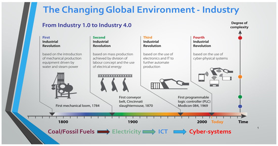
Figure 1.
The evolution of industrial revolutions over time (DUT Inaugural Lecture).
In the 1970s, it was believed that automating repetitive tasks would liberate people, resulting in more free time and less working time [1]. Despite advancements in technology, this promise remained mostly unmet [1,2]. Now, the Fourth Industrial Revolution, which builds on digitalization and information and communication technologies (ICT), is thought to be revolutionizing everything [6]. It is projected that new technologies including artificial intelligence (AI), biotechnology, the Internet of Things (IoT), quantum computing, and nanotechnology will alter how we interact with one another, perform our jobs, run our economies, and even “the mere meaning of being a human being” [7]. It should be noted that the definition of the Fourth Industrial Revolution employed in this paper brightens a technology-centric understanding of 4IR; however, one should bear in mind the other important factors including the implications for society, politics, law, and ethics. Even though 4IR has been the topic of discussion on many international forums, there have not been many systematic attempts to analyze the state of the art of this new industrial revolution wave [6]. This situation may be more apparent in Africa, where the Third Industrial Revolution has mostly not even fully begun [1,2,3]. Therefore, African academics have expressed skepticism and caution regarding the alleged advantages of information and communications technology (ICT) in African environments. Swaminathan [8] stated the following:
“Such a dream of transforming an agro-based economy into an information society must either be a flight of fancy or thinking hardly informed by the industrial economic background of developed economies that are in transition to informational economies. For an economy with about half of its adult population engaged in the food production sector, and about 70% of its development budget sourced from donor support, any talk of transition into an information society sounds like a far-fetched dream [8]”.
Monzurul [9] argued that one cannot leap into the information age. Although African leaders and officials have spoken out in support of 4IR’s goals, most of the continent’s nations continue to be heavily dependent on an agrarian economy [10]. Pachade [5] stated that critics frequently advocate that some community ICT projects have been unsuccessful partly because of the technology/reality divide. Africa has previously been described as a technological and digital wilderness [3,10,11]. It is evident that Africa still lags the rest of the international community regarding the Fourth Industrial Revolution. This is due to several factors such as poor infrastructure and over-reliance on the primary sector—agriculture [6].
Agriculture remains the backbone of the African continent; it is a crucial part of the global economy and plays an important role in providing food for the rapidly growing population and hence its heightened food demand [8,10]. According to the United Nations, the world’s population is anticipated to reach over 10 billion people by 2050, virtually doubling global food consumption [3]. Therefore, global agricultural productivity will need to rise by 1.75% each year to meet the resulting food demand [3,11]. The Global Harvest Initiative (GHI) estimated that productivity is currently increasing at a rate of 1.63% annually since the farmers are already being assisted by precision agriculture and advanced technologies such as automation, machine learning, computer vision, and artificial intelligence in keeping up with the food demand [5]. Global navigation satellite systems (GNSSs) are playing a particularly significant role as enablers in the transformation of the agricultural sector through precision agriculture.
Prashar [12] defined precision agriculture as a smart form of farm governance using digital systems, sensors, microcontrollers, actuators, robotics, and communication systems to achieve the goals of sustainability, revenue, and environmental conservation. Swaminathan [8] defined it as the integration of different computer tools into conventional agricultural methods to maximize the farm harvest and achieve self-sufficiency in farming operations. Precision agriculture (also known as digital farming or intelligent agriculture) includes (but is not limited to) the following: pest detection, weed detection, plant disease detection, morphology, irrigation monitoring and control, soil monitoring, air monitoring, humidity monitoring, and harvesting [4,6,7,8,12]. This paper aimed to study in detail the recent research trends in precision agriculture—particularly in the disease/pest/weed detection area—to comprehend the artificial intelligence (AI) tools and scientific background required to implement these machine learning (ML)-based precision agriculture systems.
The disease/pest/weed detection system was chosen because it possesses a multipurpose architecture that can be applied in several diverse applications on a farm with only amendments to the software and limited changes to the hardware; for example, a disease, weed, pest, nutrient deficiency, or morphological feature. Detection systems all have similar working principles in which a high-quality picture is acquired from a farm specimen, and an ML algorithm is then fed that picture after processing to classify what it detected in the given picture. Therefore, these systems can have similar prototypic architectures, and a farmer can have one universal robotic system that has a few changeable parts (such as cameras and sensors) and different software that are specific to different activities. This paper aimed to present and summarize the recent research trends in precision agriculture—particularly in the disease/pest/weed detection area—to identify the opportunities for further research. Its general architecture can be seen in Figure 2. The following research questions were addressed in this study:
- What are the recent precision agriculture research developments, particularly for disease/pest/weed detection systems?
- What are the found limitations and gaps in the literature review?
- What are the arising opportunities for further research?
- Lastly, what topological amendments can be made to the traditional precision agricultural systems to make them more economical to employ in rural farms and make them more accessible?

Figure 2.
The general structure of this review paper.
2. Literature Review: Precision Agriculture Research Developments
Monitoring and early identification of diseases, pests, and weeds are imperative in an effective farming operation [1]. In conventional agricultural practices, farmers rely upon visual observations of specimens to identify diseased leaves, fruits, roots, and other parts of crops [4,6]. However, this method is faced with several challenges that include the need for continuous checking and observation of specimens, which is tedious and expensive for large farms but most importantly, much less accurate [1,2,11]. Badage [1] asserted that agriculturalists often consult experts for the identification of infections of their crops, which incurs even more costs and results in longer turnaround times. The earlier-stated limitations of classical farming methods coupled with the pressure to keep up with an exponentially growing demand for food both in quantity and quality have served as the push factors for researchers to devise new strategies and tools to digitize the agricultural field with the prime objective of increasing the farm yields and produce [13]. The following subsection discusses the general plant disease detection system; one should note that the same general topology can be used to monitor pests, weeds, morphological features, and similar factors.
2.1. Plant Disease/Pest/Weed Detection System Basic Principles
Detection of diseases, pests, or weeds is achieved by utilizing machine learning (ML) [3,5,6,11,12]. Shruthi [3] defined ML as an intelligent technique in which a machine is capacitated to recognize a pattern, recall historical information, and train itself without being commanded to do so. Both supervised and unsupervised training strategies can be utilized for machine training [8]. While there are distinct training and assessment datasets for supervised training, there is no such distinction for unsupervised training datasets [12]. Prashar [12] further stated that since ML is an evolving procedure, the machine’s performance becomes better with time. As soon as the machine has finished learning or training, it may classify the data, make predictions, and even generate fresh test data from which its re-trains itself, and the process goes on and on [8]. Adekar [4] defined ML as a decision-making tool capable of visualizing the potentially complicated inter-relationships between important parameters on a farm and making educated predictions and/or decisions.
The author further provided an illustration of an ML application in precision agriculture as seen in Figure 3. In the three-level precision agricultural layout shown, the first level, which is the physical layer, represents all the field equipment such as sensors, trackers, actuators, and probes that are in physical contact with the farm environment and are collecting data for further processing [4]. In the second level, the edge layer is where the processing of the data collected in Level 1 is taking place to convert the raw data into useful information that is used to inform the decision making. The decision making takes place at this level through computational tools such as computers, microcontrollers, microprocessors, and similar ones [4]. In the third level (the cloud layer), the storage of data for iterative training of the machine takes place [4]. Therefore, the plant disease detection system is made up of two main subsystems, viz. the image-processing system and the classification system. The image processing is further subdivided into four steps. The four most cited different classification protocols are summarized in Table 1.
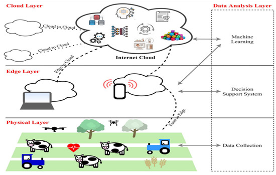
Figure 3.
Format of precision agriculture system [4].

Table 1.
Summary of image-processing steps and different classification techniques in plant disease detection.
The latest studies of phenomics and high-throughput picture-data gathering are available; however, most of the research on image interpretation and processing can be found in textbooks that dive into extensive detail into the methodologies [14]. Figure 4 summarizes the techniques for image acquisition and processing generally utilized for plant disease detection systems.
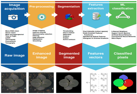
Figure 4.
Steps of image processing [5].
2.1.1. Image Processing
Image Acquisition
Image collection is the first step in a system for detecting plant diseases [6,8,12]. Image sensors, scanners, and unmanned aerial vehicles (UAVs) can all be used to capture photos of plants [3]. The commonly utilized image-acquisition tools are a charge-coupled device (CCD) and a complementary metal–oxide–semiconductor (CMOS) [15]. Both of these camera technologies convert light signals and protons to digital data, which is then further transformed into a picture [15,16]. However, their methods of turning the light signals into image data vary [16]. In a CCD camera, the light signals are transferred through a series of adjacent pixels before being amplified and converted into image data at the end of these pixel strings [17,18]. This enables CCD cameras to possess minimal degradation during the image-acquisition process [19]. CCD cameras generate sharp pictures with reduced distortion [18]. Contrarily, in CMOS cameras the light signals are collected, amplified, and converted at each pixel of the image sensor [15]. This enables the CMOS devices to generate images faster than CCD devices since each pixel can convert light signals into an image locally [17]. CMOS devices are normally preferred in projects with a low budget since they are cheap compared to CCD devices, have a lower power consumption, and can acquire high-quality images faster than their CCD counterparts [17,18,19]. Figure 5 shows the serial versus localized pixel image conversion of CCD and CMOS image sensors, respectively.
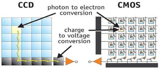
Figure 5.
CCD vs. CMOS image conversion [15].
An imaging acquisition tactic known as time delay and integration (TDI) can be combined with either CCD or CMOS technology to drastically improve their image-acquisition capabilities [20]. Applications involving fast-moving objects and requiring high precision and the capacity to function in extremely dim lighting environments use TDI [20,21]. Refer to Figure 6 for an example of a high-speed application of TDI technology in which a high-velocity train was captured with a normal and a TDI-featured camera in the left and right pictures, respectively. When the camera was operated in normal mode, the image of the train was a blur due to its high velocity and dim lighting conditions; however, the incorporation of a TDI mode countered these challenges and produced a clear detailed picture of the train.
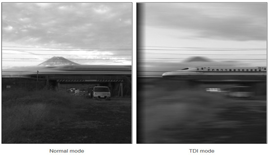
Figure 6.
Impact of TDI incorporation in CMOS and CCD sensors [5].
After an image has been captured with a CCD or CMOS device with or without TDI technology incorporated, the captured image should proceed to the following step of the image processing, which is normally image segmentation [3,5,11,12,16]. The segmentation of an image is a process in which the features of interest are extracted from the rest of the image and irrelevant features are masked [10]. The features of interest are referred to as the foreground, while the irrelevant ones are referred to as the background [16]. The creation of the foreground versus background is dependent on picture properties such as color, spectrum brightness, edge detection, and neighbor resemblance [17]. However, image pre-processing may occasionally be necessary before an effective image segmentation can take place [3,8,11,22].
Image Pre-Processing
This is a crucial step in an ML-based disease detection system [14]. Pre-processing of an image deals with the correct setting of image contrast and filtration of interference signals resulting in noise and hence blurry images [18,19]. This procedure can greatly enhance the precision of feature extraction and the correct disease detection in general [15]. Pre-processing typically involves straightforward treatments such as image cutting, clipping, cropping, filtering, trimming, and deblurring [3]. Wang [23] explained that a typical image pre-processing procedure that is generally employed in image-based detection systems comprises image acquisition, gray scaling, filtering, binarization, and edge filtering.
The first step in the procedure illustrated in Figure 7 involves the transformation of a colored image into a gray image [23]. This conversion stage into a gray image may be omitted in applications in which color features are of relevance; otherwise, this step is crucial because it is much simpler and faster to process an image in a gray color format [17]. The second stage involves the denoising of a specimen image because in most cases, images are not without interference with the noise signal, which affects the visibility of the features in the specimen images [23]. The third step then includes image segmentation, which will be explained more broadly in the coming Section. The last step involves the forming of an outline image, which can be achieved by masking the leafstalk as well as holes while keeping the outer connected region [15,23]. Wakhare [24] proposed a similar procedure to that illustrated in Figure 7 for plant-leaf feature identification applications under real-life varying lighting conditions. This procedure involves the conversion of a specimen image into grayscale, noise suppression as well as smoothing, and formation of the image outline through edge filtering. In a comparative study conducted by Ekka [25], a histogram equalization method was proven to be the most effective form of image enhancement of the gray images that were originally color images. Conversely, Kolhalkar [26] found that red–green–blue (RGB) camera images offer more valuable image enhancement compared to those converted to grayscale in the context of identifying diseases on the plant leaves.
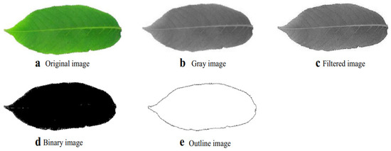
Figure 7.
General pre-processing procedure for plant-based feature-detection systems [23].
Therefore, we could not conclude which image pre-processing technique is better than the other, rather the application in which the image is used, and thing kind of image involved in that application shall be considered in the selection of an appropriate pre-processing technique.
Image Segmentation
Image segmentation is a pivotal part of image-based plant feature identification and phenotyping systems [23]. Segmentation of an image involves the separation between the foreground and the background [15]; that is, the isolation of the feature of interest and masking of the irrelevant part of the image [24,25,26]. The features of interest are normally identified by comparing adjacent pixels for similarity by looking at the three main parameters, viz. the texture, color, and shape [15,17]. Table 2 shows a list of free data libraries available to the public for use in the image segmentation process.
Table 2.
Table showing a list of image segmentation ML libraries.
A very popular example of an image segmentation technique is thresholding [55]. Threshold segmentation is a process of converting a color or grayscale image into a binary image (as shown in Figure 8) with the sole purpose of making feature classification easier [55,56]. The output binary images consist of black and white colored pixels that correspond to the background and foreground, respectively, or vice versa [26,55,56].
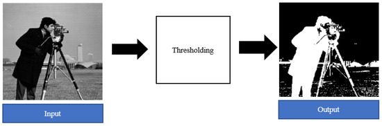
Figure 8.
Example of thresholding image segmentation [26].
Threshold segmentation is mathematically defined as follows, where T refers to a certain threshold intensity, g is the black or white pixel of a binary image, and f is the gray level of the input picture [56]:
Threshold segmentation is subdivided into global, local, and adaptive thresholding [15,57]. Global thresholding is applied in scenarios where there is enough distribution between the intensity distribution of the foreground compared to the background [15]. Hence, a single threshold value is selected and used to distinguish between the features of significance and the background [15,55]. Local thresholding is applied in cases where there is no distinct difference in intensity distribution between the background and the foreground and hence it is not conducive to selecting a single threshold value [55]. In such a case, an image is partitioned into smaller images, and different threshold values for each partitioned picture are selected [15]. Adaptive thresholding is also appropriate for images with uneven intensity distribution because a threshold value is calculated for each pixel [57]. The Otsu thresholding method is another thresholding technique used for image segmentation [15]. In this technique, a measure of spread for the pixel intensity levels on either side of the threshold is listed by looping through all the reasonable threshold values [58]. The intent is to decide the threshold value for which the summation of foreground and background escalates is at its minimum [15,58]. The fundamental characteristic of the Otsu thresholding method is the fact that it implements the threshold values automatically instead of it being preselected by the user [58]; (2) below shows the mathematical definition for the thresholding in the Otsu method.
Another segmentation method applied in image processing is watershed transformation [59]. A grayscale image undergoes a transition called a watershed [59,60]. In a metaphorical sense, the name alludes to a geologic catchment or drainage split that divides parallel catchments [59]. The watershed conversion locates the lines that follow the tops of ridges by treating the image it operates upon as a topographic map; the luminosity of each pixel denotes its elevation [60]. Figure 9 is an example of a watershed-segmented image in which the black pixels denote the background, the gray pixels denote the features to be extracted, and the white pixels correspond to watershed lines [61].
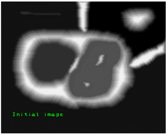
Figure 9.
Watershed image segmentation example [61].
On the other hand, Grabcut is a very popular and innovative segmentation technique that takes into consideration the textural and boundary conditions of an image [62]. This segmentation method is based on the iterative graph-cut method in which a mathematical function is derived to implement the background as well as the foreground [63]. Each pixel in an image is then assessed to decide whether it falls in the background or the foreground [62,63]. The Grabcut segmentation method is preferred in most applications because of minimal user interference in the operation of this technique; however, it is not without its drawbacks [62]. The Grabcut sequence cycles take a long time to implement because of the complexity of the thresholding equation [63]. The segmentation is also poor in scenarios where the background is complex and there is minimal distinction between the features of interest and the background [64]. Several distinct segmentation methods and algorithms exist in the literature. The suitability of a particular method is based on a particular application, and hence this study was not able to rule out certain segmentation methods or determine which ones outperform the others.
Feature Extraction
One of the foundational elements of computer-vision-based image recognition is the extraction of features [65]. A feature is data that are utilized to solve a particular computer vision problem and is a constituting part of a raw image [64]. The feature vectors include the features that have been retrieved from an image [66]. An extensive range of techniques is used to identify the items in an image while creating feature vectors [62]. Edges, image pixel intensity, geometry, texture, and image modifications such as Fourier, Wavelet, or permutations of pixels from various color images are the primary features [46,66]. Use as a set of classifiers and machine learning algorithms is feature extraction’s ultimately purpose [66]. The feature extraction in plant leaf disease-monitoring systems is subdivided into three spheres that include texture, color, and shape [20,21,46,65].
- Shape Features
The shape is a basic characteristic of a leaf used in feature extraction of leaf images during image processing [66]. The primary shape parameters include the length (L), which is the displacement between the two points in the longest axis; the width (W), which denotes the displacement between the shortest axis; the diameter (D), which denotes the maximum distance between the points; the area (A), which denotes the surface area of all the pixels found within the margin of a leaf picture; and the perimeter (P), which denotes the accumulative length of the pixels around the margin of a leaf picture [55,58,62,64]. From the 5 defined primary characteristics of shape features, 11 distinct secondary features are formed by mathematical definitions involving 2 or more primary variables [59]. These 11 features are called the morphological features of a plant. The morphological features are as follows:
- Circularity (C)—a feature defining the degree to which a leaf conforms to a perfect circle. It is defined as [60]:
- Rectangularity (R)—a feature defining the degree to which a leaf conforms to a rectangle. It is defined as [55]:
- Aspect ratio (AS)—ratio of width to length of a leaf. It is defined as [55]:
- Smooth factor (SF)—ratio of leaf picture area when 5 × 5 and 2 × 2 regular smoothing filters have been used [58].
- Perimeter-to-diameter ratio (PDr)—ratio of the perimeter to the diameter of a leaf. It is defined as [64]:
- Perimeter to length plus width ratio (PLWr)—ratio of the perimeter to length plus width of a leaf. It is defined as [64]:
- Narrow factor (NFr)—ratio of diameter to length of a leaf [60]:
- Area convexity (ACr)—area ratio between the area of a leaf and the area of its convex hull [59].
- Perimeter convexity (ACr)—the ratio between the perimeter of a leaf to that of its convex hull [60].
- Eccentricity (Ar)—the degree to which a leaf shape is a centroid [64].
- Irregularity (Ir)—ratio of the diameters of an inscribed to the circumscribed circles on the image of a leaf [59].
- Color Features
Other researchers and scholars chose to implement the color features as the pivotal features during the extraction process [67]. The color features normally cited in the literature on leaf feature extraction include the following:
- Color standard deviation (σ)—a measure of how much the different colors found in an image match one another or are rather different from one another [60]. If an image is differentiated into an array of its basic building blocks (the pixels), then i is a pointer moving across the rows of pixels in an array from the origin to the very last row M, while j is a pointer moving across the columns of pixels in an array from the origin to the very last column N. At any point, a pixel color intensity is defined by p(i, j), where i and j denote the coordinate position of a pixel in an image array. Therefore, the color standard deviation is mathematically defined as follows:
- Color mean (μ)—a measure to identify a dominant color in a leaf image. This feature is normally used to identify the leaf type [63]. It is mathematically defined as follows:
- Color skewness (φ)—a measure to identify a color symmetry in a leaf image [21,46]:
- Color kurtosis (φ)—a measure to identify a color shape dispersion in a leaf image [65]:
- Texture Features
There are also several textural features referenced by authors such as Singh [68], Martsepp [69], and Ponce [70]. Using the same assumption of an image partitioned into pixels in the above Section, the following are the textural features used for feature extraction in plant leaves:
- Entropy (Entr)—this is a measure of the complexity and uniformity of a texture of a leaf image [68]:
- Contrast (Con)—this is a measure of how clear the features are in a leaf image; it is also referred to as the moment of inertia [69,70]:
- Energy (En)—this is a measure of the degree of uniformity of a gray image. It is also called the second moment [69]:
- Correlation (Cor)—this is a measure of whether there is a similar element in a sample picture that corresponds to the re-occurrence of a similar matrix within a large array of pixels [68].
- Difference moment inverse (DMI)—this is a measure of the degree of homogeneity in an image [69]:
Other textural features include the maximum probability, which is the highest response to correlation; the standard deviation and/or variance, which is the aggregate texture observed in a leaf picture; and the average illuminance, which is the average light distribution across the leaf when an image was captured [66,68,69,70]. The selection of a particular color, shape, or textural feature strictly depends on the application of the system being designed.
2.1.2. Feature Classification
The classification techniques are machine learning algorithms that are used to categorize input sample data into different classes or groups of belonging or membership [3,5,11,56]. These classifiers may employ supervised learning, unsupervised learning, and reinforcement learning methods during their training [39]. Supervised learning occurs when a person is a trainer of the model and may use pre-formed datasets to conduct the training [39,53]. Unsupervised learning occurs when there is no training data available and the algorithm must train itself and improve its classification efficiency by iteratively adjusting itself [5,39,53]. Reinforcement learning occurs when the algorithm makes classification rulings based on the feedback applied by the environment to it [12,39]. In the case of vision-based plant disease-monitoring systems, the most cited classification algorithms include support vector machines (SVM), artificial neural networks, k-nearest neighbors’ machines, and fuzzy machines. The following subsections discuss these classification techniques.
SVM Classifier
The support vector machine, sometimes known as SVM, is a predictive model used to solve both regression and classification tasks [3]. It is a supervised learning model that works well for numerous practical problems and can solve both linear and non-linear tasks [3,71]. The SVM concept is relatively simple; a vector or a hyperplane that splits the data into groups is generated by this technique [72].
In Figure 10, the optimal hyperplane is used to separate the two classes of data (the blue squares and green circles). The two planes (dashed lines) parallel to the optimal hyperplane are called the positive and negative imaginary planes, which are the planes passing through the closest data points to either side of an optimal hyperplane [72]. These closest points to the optimal hyperplane are called the support vectors and are used to determine the exact position of an optimal hyperplane [73]. There might be several possible hyperplanes, but the optimal hyperplane is the one with the maximum marginal distance, which is the distance between the two marginal planes [72,73]. The maximized margin results in a more generalized solution compared to smaller margins; should the training data change, the algorithm with a smaller margin will have accuracy challenges [73]. In some cases, data classes are not always easily separable with a straight line or place as in the case of Figure 10. Therefore, when data classes show a property of non-linearity, transforming a space in which these data classes occur from a low-dimension (often two-dimensional) into a high-dimension space (often three-dimensional) space using the kernel method. The kernel method is a computation of a dot product of the dimensions in the new high-dimension space [72,73,74]; (17) below gives the general solution of a hyperplane, where is any data point or support vector, is the weight vector that applies the bias of the support vectors, and is the constant [74].
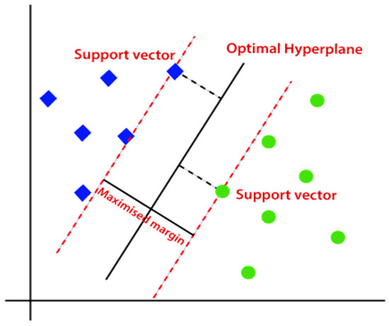
Figure 10.
SVM classification algorithm [72].
ANN Classifier
An ANN is a supervised learning model that is a collection of interlinked input and output nodes in which each link has an associated bias value called a weight [75]. A single input layer, one or perhaps more intermediate layers that are normally called hidden layers, and one or more output layers make up the structure of an ANN [75,76]. The weight of each connection is modulated as the network operates to facilitate neural network learning [76]. The performance of the network is enhanced by adjusting the weight continuously [75]. ANN can be divided into two groups based on connection types: feed-forward networks and recurrent networks [33]. In contrast to recurrent neural networks, feed-forward neural networks do not have cycle-forming connections between units [76]. The architecture, transfer function, and learning rule all have an impact on how a neural network behaves [49,76]. The weighted total of input triggers the activation of neural network neurons [75]. Figure 11 shows a generalized model of an ANN model with the input layer, the hidden intermediate layer (purple layer), and the output layer.
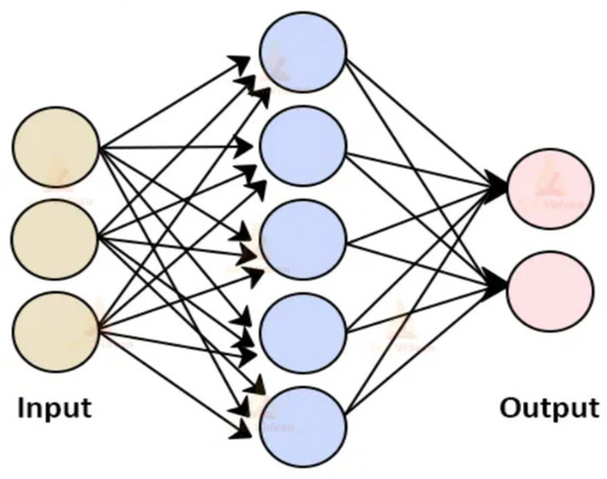
Figure 11.
ANN model architecture [77].
k-NN Classifier
The k-nearest neighbors algorithm, sometimes known as k-NN, is the most straightforward machine learning technique [78]. It is a non-parametric technique used for problems involving regression and classification [74,78]. Non-parametric implies that no dataset for initial training is necessary [78]. Therefore, k-NN does not require the use of any presumptions [79]. The k-closest training examples in the feature space provide the input for classification and regression tasks, respectively [78]. Whether k-NN is applied for classification or regression determines the results [79]. The outcome of the k-NN classifier is a class of belonging [74,78,79]. Based on the predominant kind of its neighborhood, the given data point is classed [79]. The input point is awarded to the category that has the highest frequency among its k-closest neighbors [78]. In most cases, k is a small positive integer such as 1. The result of a k-NN regression is just a value of the property for the attribute. The aggregate of the variables of the k-closest neighbors constitutes this number [79].
Figure 12 shows a space with numerous data points or vectors that can be classified into two classes: the red class and the green class. Now, assume there exists a data point at any location in the space shown in Figure 12 that is unknown whether it belongs to either the red or green class. The k-NN will then proceed through the following computational steps to assign that point a class of belonging:
- Take the uncategorized data point as input to a model.
- Measure the spatial distance between this unclassified point to all the other already classified points. The distance can be computed via Euclidean, Minkowski, or Manhattan formulae [80].
- Check the points with the shortest displacement from the unknown data point to be classified for a certain K value (K is defined by the supervisor of the algorithm) and separate these points by the class of belonging [80].
- Select the correct class of membership as the one with the most frequent vectors as the neighbors of the unknown data point [80].

Figure 12.
Classification principle of a k-NN model [80].
The most cited method of computing the spatial distance between the data point p to be classified and its neighbors qn is the Euclidean Formulae (18) [74,80]:
Fuzzy Classifier
The fuzzy classifier system is a supervised learning model that enables computational variables, outputs, and inputs to assume a spectrum of values over predetermined bands [81]. By developing fuzzy rules that connect the values of the input variables to internal or output variables, the fuzzy classifier system is trained [82]. It has mechanisms for credit assignment and conflict resolution that combine elements of typical fuzzy classifier systems [81]. A genetic algorithm is used by the fuzzy classifier system to develop suitable fuzzy rules [83].
As shown in Figure 13, fuzzy sets display a continuous membership, and a data point membership classification can be ruled as the extent (μ) to which it belongs to a certain fuzzy set. For example, 690 mm in Figure 13 has a degree of membership μ(960) on the close fuzzy set that is 0.7. It can also be seen in Figure 9 that a data point can belong to multiple fuzzy sets, and the degrees of membership to each set may or may not (in the intersection points) differ since some fuzzy sets overlap with each other. Table 3 summarizes the advantages and disadvantages of all the classification techniques discussed in this section.
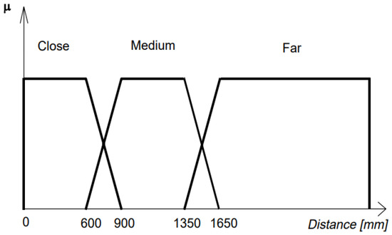
Figure 13.
Example of fuzzy sets for classification [83].
Table 3.
Table showing pros and cons of different classification methods.
2.2. Literature Survey: Plant Disease/Nutrient Deficiency Monitoring Systems
Many authors in the literature have proposed plant disease/pest/weed detection systems that employ the above-described general format. Literature shows that this technology of plant disease detection models has been developing at a faster rate in the last two decades and achieving high success in terms of classification accuracy and efficiency.
2.2.1. Tabulated Summary of Plant Disease/Nutrient Deficiency Monitoring Systems publications
Table 4 summarizes a literature survey on these systems. Several publications have been consulted for this research study. A few aspects have been noted for each publication such as the type of crop investigated, the number of crop disease covered in the study and the classification results achieved.
Table 4.
Summary of a literature survey on plant disease/pest/weed detection systems.
2.2.2. Research Opportunities Identified
- During the literature survey presented in earlier sections, the following opportunities that the authors of this paper believe have seen little interest from researchers are as follows:
- Little discussion of the real-time monitoring of the onset signs of diseases before they spread throughout the whole plant.
- Few papers discussed real-time monitoring and real-time mitigation measures such as actuation operations, spraying pesticides, and spraying fertilizers, to name a few examples.
- Very little research discussed the combination of these monitoring and phenotyping tasks into one system to reduce costs and improve technology availability to farmers and add convenience.
- Little research discussed the post-harvest benefits of disease/nutrient deficiency detection or similar systems.
- Most research papers on plant disease detection models processed two-dimensional images captured from plant samples. In cases where samples were in the form of fruits, single-input cameras or a two-dimensional view may pose a challenge because of the spherical or cylindrical nature of most fruits. The authors noticed that the fruit disease symptoms or any types of defects are not always evenly distributed across the surface area of a sample fruit; Figure 14 shows an example. Therefore, in high-throughput and high-speed applications, a sample fruit might be oriented such that the diseased part is masked or hidden from the camera’s line of sight, so an incorrect classification is highly probable.

Figure 14.
A sample fruit with uneven distribution of the disease-infected surface area.
- Few studies discussed the importance of optimum optical or lighting conditions in the successful operation of an image-based plant disease detection model and their relationship to classification accuracy and efficiency.
Hence, this study took advantage of the second-to-last opportunity outlined above and proposes two conceptual ideas as a mitigation measure. The purpose of these two propositions is to give a classification model a virtual three-dimensional view of a sample fruit so that a classification model “sees” the total surface of a sample fruit so as not to miss any important details before making a final classification. The two proposed ideas are:
- A multicamera-input fruit disease detection model
- A dynamic-input fruit disease detection model
A multicamera-input fruit disease detection model has an improved input system that features multiple-input camera sensors specially arranged in a circular setup and equidistant from each other with a sample fruit at the central point. These cameras capture the surface of a sample fruit at different angles such that all the fruit surface is captured (refer to Figure 15).
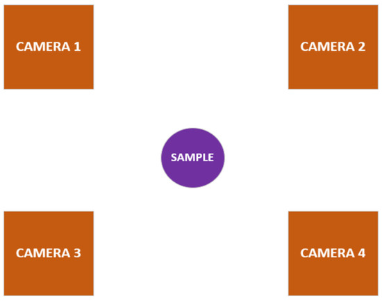
Figure 15.
Multicamera-input setup.
The classification model should classify each input image from each camera independently and consolidate all the results to make a final classification. The final classification should be decided as follows:
- If at least one input image is classified as a diseased sample, set the final classification to a “diseased sample”.
- Otherwise, set the final classification to a “healthy sample”.
A dynamic input fruit disease detection model, on the other hand, maintains a single-input camera but instead features a revolving sample stand that rotates in steps of a predetermined angle ϴ while an input image is captured per rotation until the full circumference of a sample fruit has been captured (refer to Figure 16).
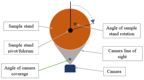
Figure 16.
A dynamic input design for the fruit disease detection system.
All the capture samples are processed similarly as in the multicamera input disease detection mode. The authors foresee that these two may have different pros and cons such as the classification cycle time per each sample; however, this still needs to be examined in more detail.
3. Conclusions
This paper has presented the background on the research developments in plant disease detection models for agricultural applications. Substantial progress has been achieved in this research area, several crops have been considered, and several disease or nutrient detection models have been proposed that are capable of classifying each with no less than 75% accuracy as presented in the literature survey section of this paper. This study has found image processing and machine learning to be the widely used tools amongst a large proportion of researchers to implement plant disease or nutrient detection models.
This study also presented a few opportunities that the authors believe are worth further research (presented in Section 2.2.2) and has proposed two separate improvements that can be made to the classical disease classification models to improve the classification accuracy and efficiency. Much more can still be done to further improve the accuracy levels of some monitoring systems presented in Table 4 such as improving the training data. This study is already serving as a foundation for a Doctor of Philosophy Research Project that seeks to explore some of the research opportunities presented in this paper.
Author Contributions
Conceptualization, M.S.P.N.; methodology, M.S.P.N.; software, M.S.P.N.; validation, M.S.P.N., M.K. and K.M.; formal analysis, M.S.P.N.; investigation, M.S.P.N.; resources, M.K. and K.M.; data curation, M.S.P.N.; writing—original draft preparation, M.S.P.N.; writing—review and editing, M.K. and K.M.; visualization, M.K. and K.M.; supervision, M.K. and K.M.; project administration, M.S.P.N.; funding acquisition, M.K. All authors have read and agreed to the published version of the manuscript.
Funding
This research was self-funded, and the APC was funded by Musasa Kabeya.
Data Availability Statement
This research study is a review paper and hence no data was created but a few research ideas were conceptualized. Any data regarding any contents of this paper will be made available upon request.
Conflicts of Interest
The authors declare no conflict of interest.
References
- Badage, A. Crop disease detection using machine learning: Indian agriculture. Int. Res. J. Eng. Technol. 2018, 5, 866–869. [Google Scholar]
- Ukaegbu, U.; Tartibu, L.; Laseinde, T.; Okwu, M.; Olayode, I. A deep learning algorithm for detection of potassium deficiency in a red grapevine and spraying actuation using a raspberry pi3. In Proceedings of the 2020 International Conference on Artificial Intelligence, Big Data, Computing and Data Communication Systems (icabcd), Durban, South Africa, 6–7 August 2020; IEEE: New York, NY, USA, 2020; pp. 1–6. [Google Scholar]
- Shruthi, U.; Nagaveni, V.; Raghavendra, B. A review on machine learning classification techniques for plant disease detection. In Proceedings of the 2019 5th International Conference on Advanced Computing & Communication Systems (ICACCS), Coimbatore, India, 15–16 March 2019; IEEE: New York, NY, USA, 2020; pp. 281–284. [Google Scholar]
- Park, H.; Eun, J.; Se-Han, K. Crops disease diagnosing using image-based deep learning mechanism. In Proceedings of the 2018 International Conference on Computing and Network Communications (CoCoNet), Astana, Kazakhstan, 15–17 August 2018; pp. 23–26. [Google Scholar]
- Dharmasiri, S.B.D.H.; Jayalal, S. Passion fruit disease detection using image processing. In Proceedings of the 2019 International Research Conference on Smart Computing and Systems Engineering (SCSE), Colombo, Sri Lanka, 28 March 2019; IEEE: New York, NY, USA, 2019. [Google Scholar]
- du Preez, M.-L. 4IR and Water Smart Agriculture in Southern Africa: A Watch List of Key Technological Advances; JSTOR: Ann Arbor, MI, USA, 2020. [Google Scholar]
- Hoosain, M.S.; Paul, B.S.; Ramakrishna, S. The impact of 4IR digital technologies and circular thinking on the United Nations sustainable development goals. Sustainability 2020, 12, 10143. [Google Scholar] [CrossRef]
- Swaminathan, B.; Barrett, T.J.; Hunter, S.B.; Tauxe, R.V.; Force, C.P.T. PulseNet: The molecular subtyping network for foodborne bacterial disease surveillance, United States. Emerg. Infect. Dis. 2001, 7, 382. [Google Scholar] [CrossRef]
- Islam, M.; Wahid, K.A.; Dinh, A.V.; Bhowmik, P. Model of dehydration and assessment of moisture content on onion using EIS. J. Food Sci. Technol. 2019, 56, 2814–2824. [Google Scholar] [CrossRef]
- Anju, S.; Chaitra, B.; Roopashree, C.; Lathashree, K.; Gowtham, S. Various Approaches for Plant Disease Detection; Acharya: Bengaluru, India, 2021. [Google Scholar]
- Swain, S.; Nayak, S.K.; Barik, S.S. A review on plant leaf diseases detection and classification based on machine learning models. Mukt Shabd 2020, 9, 5195–5205. [Google Scholar]
- Prashar, N. A Review on Plant Disease Detection Techniques. In Proceedings of the 2021 2nd International Conference on Secure Cyber Computing and Communications (ICSCCC), Jalandhar, India, 21–23 May 2021; IEEE: New York, NY, USA, 2020; pp. 501–506. [Google Scholar]
- Agrawal, N.; Singhai, J.; Agarwal, D.K. Grape leaf disease detection and classification using multi-class support vector machine. In Proceedings of the 2017 International Conference on Recent Innovations in Signal processing and Embedded Systems (RISE), Bhopal, India, 27–29 October 2017; IEEE: New York, NY, USA, 2020; pp. 238–244. [Google Scholar]
- Dar, Z.A.; Dar, S.A.; Khan, J.A.; Lone, A.A.; Langyan, S.; Lone, B.; Kanth, R.; Iqbal, A.; Rane, J.; Wani, S.H. Identification for surrogate drought tolerance in maize inbred lines utilizing high-throughput phenomics approach. PLoS ONE 2021, 16, e0254318. [Google Scholar] [CrossRef] [PubMed]
- Perez-Sanz, F.; Navarro, P.J.; Egea-Cortines, M. Plant phenomics: An overview of image acquisition technologies and image data analysis algorithms. GigaScience 2017, 6, gix092. [Google Scholar] [CrossRef] [PubMed]
- Padmavathi, K.; Thangadurai, K. Implementation of RGB and grayscale images in plant leaves disease detection—Comparative study. Indian J. Sci. Technol. 2016, 9, 1–6. [Google Scholar] [CrossRef]
- Kern, T.A. Application of Positioning Sensors. In Engineering Haptic Devices: A Beginner’s Guide for Engineers; Springer: Berlin/Heidelberg, Germany, 2019; pp. 357–372. [Google Scholar]
- Magazov, S.S. Image recovery on defective pixels of a CMOS and CCD arrays. Inf. Tekhnologii I Vychslitel’nye Sist. 2019, 3, 25–40. [Google Scholar]
- Defrianto, D.; Shiddiq, M.; Malik, U.; Asyana, V.; Soerbakti, Y. Fluorescence spectrum analysis on leaf and fruit using the ImageJ software application. Sci. Technol. Commun. J. 2022, 3, 1–6. [Google Scholar]
- Netto, A.F.A.; Martins, R.N.; De Souza, G.S.A.; Dos Santos, F.F.L.; Rosas, J.T.F. Evaluation of a low-cost camera for agricultural applications. J. Exp. Agric. Int. 2019, 32, 1–9. [Google Scholar] [CrossRef]
- Maddikunta, P.K.R.; Hakak, S.; Alazab, M.; Bhattacharya, S.; Gadekallu, T.R.; Khan, W.Z.; Pham, Q.-V. Unmanned aerial vehicles in smart agriculture: Applications, requirements, and challenges. IEEE Sens. J. 2021, 21, 17608–17619. [Google Scholar] [CrossRef]
- Trivedi, J.; Yash, S.; Ruchi, G. Plant leaf disease detection using machine learning. In Emerging Technology Trends in Electronics, Communication and Networking, Proceedings of the Third International Conference, ET2ECN 2020, Surat, India, 7–8 February 2020; Revised Selected Papers 3; Springer: Singapore, 2020. [Google Scholar]
- Wang, H.; Shang, S.; Wang, D.; He, X.; Feng, K.; Zhu, H. Plant disease detection and classification method based on the optimized lightweight YOLOv5 model. Agriculture 2022, 12, 931. [Google Scholar] [CrossRef]
- Wakhare, P.B.; Neduncheliyan, S.; Thakur, K.R. Study of Disease Identification in Pomegranate Using Leaf Detection Technique. In Proceedings of the 2022 International Conference on Emerging Smart Computing and Informatics (ESCI), Pune, India, 9–11 March 2022; IEEE: New York, NY, USA, 2020. [Google Scholar]
- Ekka, B.K.; Behera, B.S. Disease Detection in Plant Leaf Using Image Processing Technique. Int. J. Progress. Res. Sci. Eng. 2020, 1, 151–155. [Google Scholar]
- Kolhalkar, N.R.; Krishnan, V. Mechatronics system for diagnosis and treatment of major diseases in grape vineyards based on image processing. Mater. Today Proc. 2020, 23, 549–556. [Google Scholar] [CrossRef]
- Saleem, M.H.; Potgieter, J.; Arif, K.M. Plant disease detection and classification by deep learning. Plants 2019, 8, 468. [Google Scholar] [CrossRef]
- Contreras, X.; Amberg, N.; Davaatseren, A.; Hansen, A.H.; Sonntag, J.; Andersen, L.; Bernthaler, T.; Streicher, C.; Heger, A.; Johnson, R.L. A genome-wide library of MADM mice for single-cell genetic mosaic analysis. Cell Rep. 2021, 35, 109274. [Google Scholar] [CrossRef]
- Mazur, C.; Ayers, J.; Humphrey, J.; Hains, G.; Khmelevsky, Y. Machine Learning Prediction of Gamer’s Private Networks (GPN® S). In Proceedings of the Future Technologies Conference (FTC) 2020, Vancouver, BC, Canada, 5–6 November 2020; Springer International Publishing: New York, NY, USA, 2021; pp. 107–123. [Google Scholar]
- Vijayalakshmi, V.; Venkatachalapathy, K. Comparison of predicting student’s performance using machine learning algorithms. Int. J. Intell. Syst. Appl. 2019, 11, 34. [Google Scholar] [CrossRef]
- Adewole, K.S.; Akintola, A.G.; Salihu, S.A.; Faruk, N.; Jimoh, R.G. Hybrid rule-based model for phishing URLs detection. In Emerging Technologies in Computing, Proceedings of the Second International Conference, iCETiC 2019, London, UK, 19–20 August 2019; Proceedings 2; Springer International Publishing: New York, NY, USA, 2019. [Google Scholar]
- Krivoguz, D. Validation of landslide susceptibility map using ROCR package in R. In Proceedings of the Current Problems of Biodiversity and Nature Management, Kerch, Russia, 15–17 March 2019. [Google Scholar]
- Sieber, M.; Klar, S.; Vassiliou, M.F.; Anastasopoulos, I. Robustness of simplified analysis methods for rocking structures on compliant soil. Earthq. Eng. Struct. Dyn. 2020, 49, 1388–1405. [Google Scholar] [CrossRef]
- Aybar, C.; Wu, Q.; Bautista, L.; Yali, R.; Barja, A. rgee: An R package for interacting with Google Earth Engine. J. Open Source Softw. 2020, 5, 2272. [Google Scholar] [CrossRef]
- Wang, H.; Mou, Q.; Yue, Y.; Zhao, H. Research on detection technology of various fruit disease spots based on mask R-CNN. In Proceedings of the 2020 IEEE International Conference on Mechatronics and Automation (ICMA), Beijing, China, 13–16 October 2020; IEEE: New York, NY, USA, 2020. [Google Scholar]
- Pölsterl, S. scikit-survival: A Library for Time-to-Event Analysis Built on Top of scikit-learn. J. Mach. Learn. Res. 2020, 21, 8747–8752. [Google Scholar]
- Melnykova, N.; Kulievych, R.; Vycluk, Y.; Melnykova, K.; Melnykov, V. Anomalies Detecting in Medical Metrics Using Machine Learning Tools. Procedia Comput. Sci. 2022, 198, 718–723. [Google Scholar] [CrossRef]
- Gómez-Hernández, E.J.; Martínez, P.A.; Peccerillo, B.; Bartolini, S.; García, J.M.; Bernabé, G. Using PHAST to port Caffe library: First experiences and lessons learned. arXiv 2020, arXiv:2005.13076. [Google Scholar]
- Gevorkyan, M.N.; Demidova, A.V.; Demidova, T.S.; Sobolev, A.A. Review and comparative analysis of machine learning libraries for machine learning. Discret. Contin. Model. Appl. Comput. Sci. 2019, 27, 305–315. [Google Scholar] [CrossRef]
- Weber, M.; Wang, H.; Qiao, S.; Xie, J.; Collins, M.D.; Zhu, Y.; Yuan, L.; Kim, D.; Yu, Q.; Cremers, D. Deeplab2: A tensorflow library for deep labeling. arXiv 2021, arXiv:2106.09748. [Google Scholar]
- Kumar, M.; Pal, Y.; Gangadharan SM, P.; Chakraborty, K.; Yadav, C.S.; Kumar, H.; Tiwari, B. Apple Sweetness Measurement and Fruit Disease Prediction Using Image Processing Techniques Based on Human-Computer Interaction for Industry 4.0. Wirel. Commun. Mob. Comput. 2022, 2022, 5760595. [Google Scholar] [CrossRef]
- Essien, A.; Giannetti, C. A deep learning framework for univariate time series prediction using convolutional LSTM stacked autoencoders. In Proceedings of the 2019 IEEE International Symposium on Innovations in Intelligent Systems and Applications (INISTA), Sofia, Bulgaria, 3–5 July 2019; IEEE: New York, NY, USA, 2019. [Google Scholar]
- Pocock, A. Tribuo: Machine Learning with Provenance in Java. arXiv 2021, arXiv:2110.03022. [Google Scholar]
- Schubert, E.; Zimek, A. ELKI: A large open-source library for data analysis-ELKI Release 0.7.5 “Heidelberg”. arXiv 2019, arXiv:1902.03616. [Google Scholar]
- Zhou, C.; Ye, H.; Hu, J.; Shi, X.; Hua, S.; Yue, J.; Xu, Z.; Yang, G. Automated counting of rice panicle by applying deep learning model to images from unmanned aerial vehicle platform. Sensors 2019, 19, 3106. [Google Scholar] [CrossRef]
- Bhatia, A.; Kaluza, B. Machine Learning in Java: Helpful Techniques to Design, Build, and Deploy Powerful Machine Learning Applications in Java; Packt Publishing Ltd.: Birmingham, UK, 2018. [Google Scholar]
- Luu, H. Beginning Apache Spark 2: With Resilient Distributed Datasets, Spark SQL, Structured Streaming and Spark Machine Learning Library; Apress: New York, NY, USA, 2018. [Google Scholar]
- Vanam, M.K.; Jiwani, B.A.; Swathi, A.; Madhavi, V. High performance machine learning and data science based implementation using Weka. Mater. Today Proc. 2021. [Google Scholar] [CrossRef]
- Saha, T.; Aaraj, N.; Ajjarapu, N.; Jha, N.K. SHARKS: Smart Hacking Approaches for RisK Scanning in Internet-of-Things and cyber-physical systems based on machine learning. IEEE Trans. Emerg. Top. Comput. 2021, 10, 870–885. [Google Scholar] [CrossRef]
- Curtin, R.R.; Edel, M.; Lozhnikov, M.; Mentekidis, Y.; Ghaisas, S.; Zhang, S. mlpack 3: A fast, flexible machine learning library. J. Open Source Softw. 2018, 3, 726. [Google Scholar] [CrossRef]
- Wen, Z.; Shi, J.; Li, Q.; He, B.; Chen, J. ThunderSVM: A fast SVM library on GPUs and CPUs. J. Mach. Learn. Res. 2018, 19, 797–801. [Google Scholar]
- Kolodiazhnyi, K. Hands-on Machine Learning with C++: Build, Train, and Deploy End-to-End Machine Learning and Deep Learning Pipelines; Packt Publishing Ltd.: Birmingham, UK, 2020. [Google Scholar]
- Mohan, A.; Singh, A.K.; Kumar, B.; Dwivedi, R. Review on remote sensing methods for landslide detection using machine and deep learning. Trans. Emerg. Telecommun. Technol. 2021, 32, e3998. [Google Scholar] [CrossRef]
- Prasad, R.; Rohokale, V. Artificial intelligence and machine learning in cyber security. In Cyber Security: The Lifeline of Information and Communication Technology; Springer: Berlin/Heidelberg, Germany, 2020; pp. 231–247. [Google Scholar]
- Garcia-Lamont, F.; Cervantes, J.; López, A.; Rodriguez, L. Segmentation of images by color features: A survey. Neurocomputing 2018, 292, 1–27. [Google Scholar] [CrossRef]
- Wang, A.; Zhang, W.; Wei, X. A review on weed detection using ground-based machine vision and image processing techniques. Comput. Electron. Agric. 2019, 158, 226–240. [Google Scholar] [CrossRef]
- Ker, J.; Singh, S.P.; Bai, Y.; Rao, J.; Lim, T.; Wang, L. Image thresholding improves 3-dimensional convolutional neural network diagnosis of different acute brain hemorrhages on computed tomography scans. Sensors 2019, 19, 2167. [Google Scholar] [CrossRef]
- Kumar, A.; Tiwari, A. A comparative study of otsu thresholding and k-means algorithm of image segmentation. Int. J. Eng. Technol. Res 2019, 9, 2454–4698. [Google Scholar] [CrossRef]
- Zhang, L.; Zou, L.; Wu, C.; Jia, J.; Chen, J. Method of famous tea sprout identification and segmentation based on improved watershed algorithm. Comput. Electron. Agric. 2021, 184, 106108. [Google Scholar] [CrossRef]
- Xie, L.; Qi, J.; Pan, L.; Wali, S. Integrating deep convolutional neural networks with marker-controlled watershed for overlapping nuclei segmentation in histopathology images. Neurocomputing 2020, 376, 166–179. [Google Scholar] [CrossRef]
- Anger, P.M.; Prechtl, L.; Elsner, M.; Niessner, R.; Ivleva, N.P. Implementation of an open source algorithm for particle recognition and morphological characterisation for microplastic analysis by means of Raman microspectroscopy. Anal. Methods 2019, 11, 3483–3489. [Google Scholar] [CrossRef]
- Jadhav, S.; Garg, B. Comparative Analysis of Image Segmentation Techniques for Real Field Crop Images. In International Conference on Innovative Computing and Communications: Proceedings of ICICC 2022; Springer Nature: Singapore, 2022; Volume 2. [Google Scholar]
- Li, C.; Zhao, X.; Ru, H. GrabCut Algorithm Fusion of Extreme Point Features. In Proceedings of the 2021 International Conference on Intelligent Computing, Automation and Applications (ICAA), Nanjing, China, 25–27 June 2021; IEEE: Piscataway, NJ, USA, 2021; pp. 33–38. [Google Scholar]
- Randrianasoa, J.F.; Kurtz, C.; Desjardin, E.; Passat, N. AGAT: Building and evaluating binary partition trees for image segmentation. SoftwareX 2021, 16, 100855. [Google Scholar] [CrossRef]
- Zhu, N.; Liu, X.; Liu, Z.; Hu, K.; Wang, Y.; Tan, J.; Huang, M.; Zhu, Q.; Ji, X.; Jiang, Y. Deep learning for smart agriculture: Concepts, tools, applications, and opportunities. Int. J. Agric. Biol. Eng. 2018, 11, 32–44. [Google Scholar] [CrossRef]
- Zhang, Q.; Liu, Y.; Gong, C.; Chen, Y.; Yu, H. Applications of deep learning for dense scenes analysis in agriculture: A review. Sensors 2020, 20, 1520. [Google Scholar] [CrossRef] [PubMed]
- Ireri, D.; Belal, E.; Okinda, C.; Makange, N.; Ji, C. A computer vision system for defect discrimination and grading in tomatoes using machine learning and image processing. Artif. Intell. Agric. 2019, 2, 28–37. [Google Scholar] [CrossRef]
- Singh, S.; Kaur, P.P. A study of geometric features extraction from plant leaves. J. Sci. Comput. 2019, 9, 101–109. [Google Scholar]
- Martsepp, M.; Laas, T.; Laas, K.; Priimets, J.; Tõkke, S.; Mikli, V. Dependence of multifractal analysis parameters on the darkness of a processed image. Chaos Solitons Fractals 2022, 156, 111811. [Google Scholar] [CrossRef]
- Ponce, J.M.; Aquino, A.; Andújar, J.M. Olive-fruit variety classification by means of image processing and convolutional neural networks. IEEE Access 2019, 7, 147629–147641. [Google Scholar] [CrossRef]
- Bhimte, N.R.; Thool, V. Diseases detection of cotton leaf spot using image processing and SVM classifier. In Proceedings of the 2018 Second International Conference on Intelligent Computing and Control Systems (ICICCS), Madurai, India, 14–15 June 2018; IEEE: Piscataway, NJ, USA, 2018; pp. 340–344. [Google Scholar]
- Sandhu, G.K.; Kaur, R. Plant disease detection techniques: A review. In Proceedings of the 2019 International Conference on Automation, Computational and Technology Management (ICACTM), London, UK, 24–26 April 2019; IEEE: Piscataway, NJ, USA, 2019; pp. 34–38. [Google Scholar]
- Alagumariappan, P.; Dewan, N.J.; Muthukrishnan, G.N.; Raju, B.K.B.; Bilal, R.A.A.; Sankaran, V. Intelligent plant disease identification system using Machine Learning. Eng. Proc. 2020, 2, 49. [Google Scholar]
- Bharate, A.A.; Shirdhonkar, M. Classification of grape leaves using KNN and SVM classifiers. In Proceedings of the 2020 Fourth International Conference on Computing Methodologies and Communication (ICCMC), Erode, India, 11–13 March 2020; IEEE: Piscataway, NJ, USA, 2020; pp. 745–749. [Google Scholar]
- Sivasakthi, S.; Phil, M. Plant leaf disease identification using image processing and svm, ann classifier methods. In Proceedings of the International Conference on Artificial Intelligence and Machine Learning, Jaipur, India, 4–5 September 2020. [Google Scholar]
- Kumari, C.U.; Prasad, S.J.; Mounika, G. Leaf disease detection: Feature extraction with K-means clustering and classification with ANN. In Proceedings of the 2019 3rd International Conference on Computing Methodologies and Communication (ICCMC), Erode, India, 27–29 March 2019; IEEE: Piscataway, NJ, USA, 2019; pp. 1095–1098. [Google Scholar]
- Azadnia, R.; Kheiralipour, K. Recognition of leaves of different medicinal plant species using a robust image processing algorithm and artificial neural networks classifier. J. Appl. Res. Med. Aromat. Plants 2021, 25, 100327. [Google Scholar] [CrossRef]
- Vaishnnave, M.; Devi, K.S.; Srinivasan, P.; Jothi, G.A.P. Detection and classification of groundnut leaf diseases using KNN classifier. In Proceedings of the 2019 IEEE International Conference on System, Computation, Automation and Networking (ICSCAN), Pondicherry, India, 29–30 March 2019; IEEE: Piscataway, NJ, USA, 2019; pp. 1–5. [Google Scholar]
- Hossain, E.; Hossain, M.F.; Rahaman, M.A. A color and texture based approach for the detection and classification of plant leaf disease using KNN classifier. In Proceedings of the 2019 International Conference on Electrical, Computer and Communication Engineering (ECCE), Cox’s Bazar, Bangladesh, 7–9 February 2019; IEEE: Piscataway, NJ, USA, 2019; pp. 1–6. [Google Scholar]
- Singh, J.; Kaur, H. Plant disease detection based on region-based segmentation and KNN classifier. In Proceedings of the International Conference on ISMAC in Computational Vision and Bio-Engineering 2018 (ISMAC-CVB); Springer International Publishing: New York, NY, USA, 2019. [Google Scholar]
- Bakhshipour, A.; Zareiforoush, H. Development of a fuzzy model for differentiating peanut plant from broadleaf weeds using image features. Plant Methods 2020, 16, 153. [Google Scholar] [CrossRef] [PubMed]
- Sabrol, H.; Kumar, S. Plant leaf disease detection using adaptive neuro-fuzzy classification. In Advances in Computer Vision: Proceedings of the 2019 Computer Vision Conference (CVC); Springer International Publishing: New York, NY, USA, 2020; Volume 11. [Google Scholar]
- Sutha, P.; Nandhu Kishore, A.; Jayanthi, V.; Periyanan, A.; Vahima, P. Plant Disease Detection Using Fuzzy Classification. Ann. Rom. Soc. Cell Biol. 2021, 24, 9430–9441. [Google Scholar]
- Panigrahi, K.P.; Das, H.; Sahoo, A.K.; Moharana, S.C. Maize leaf disease detection and classification using machine learning algorithms. In Progress in Computing, Analytics and Networking; Springer: Berlin/Heidelberg, Germany, 2020; pp. 659–669. [Google Scholar]
- Singh, V.; Misra, A.K. Detection of plant leaf diseases using image segmentation and soft computing techniques. Inf. Process. Agric. 2017, 4, 41–49. [Google Scholar] [CrossRef]
- Dwari, A.; Tarasia, A.; Jena, A.; Sarkar, S.; Jena, S.K.; Sahoo, S. Smart Solution for Leaf Disease and Crop Health Detection. In Advances in Intelligent Computing and Communication; Springer: Berlin/Heidelberg, Germany, 2021; pp. 231–241. [Google Scholar]
- Tiwari, D.; Ashish, M.; Gangwar, N.; Sharma, A.; Patel, S.; Bhardwaj, S. Potato leaf diseases detection using deep learning. In Proceedings of the 2020 4th International Conference on Intelligent Computing and Control Systems (ICICCS), Madurai, India, 13–15 May 2020; IEEE: Piscataway, NJ, USA, 2020. [Google Scholar]
- Hossain, S.; Mou, R.M.; Hasan, M.M.; Chakraborty, S.; Razzak, M.A. Recognition and detection of tea leaf’s diseases using support vector machine. In Proceedings of the 2018 IEEE 14th International Colloquium on Signal Processing & Its Applications (CSPA), Penang, Malaysia, 9–10 March 2018; IEEE: Piscataway, NJ, USA, 2018; pp. 150–154. [Google Scholar]
- Coulibaly, S.; Kamsu-Foguem, B.; Kamissoko, D.; Traore, D. Deep neural networks with transfer learning in millet crop images. Comput. Ind. 2019, 108, 115–120. [Google Scholar] [CrossRef]
- Cherukuri, N.; Kumar, G.R.; Gandhi, O.; Thotakura, V.S.K.; NagaMani, D.; Basha, C.Z. Automated Classification of rice leaf disease using Deep Learning Approach. In Proceedings of the 2021 5th International Conference on Electronics, Communication and Aerospace Technology (ICECA), Coimbatore, India, 2–4 December 2021; IEEE: Piscataway, NJ, USA, 2021; pp. 1206–1210. [Google Scholar]
- Khalili, E.; Kouchaki, S.; Ramazi, S.; Ghanati, F. Machine learning techniques for soybean charcoal rot disease prediction. Front. Plant Sci. 2020, 11, 590529. [Google Scholar] [CrossRef] [PubMed]
- Prabha, D.S.; Kumar, J.S. Study on banana leaf disease identification using image processing methods. Int. J. Res. Comput. Sci. Inf. Technol. 2014, 2, 2319–5010. [Google Scholar]
- Orchi, H.; Sadik, M.; Khaldoun, M. On using artificial intelligence and the internet of things for crop disease detection: A contemporary survey. Agriculture 2021, 12, 9. [Google Scholar] [CrossRef]
- Zhang, D.; Zhou, X.; Zhang, J.; Lan, Y.; Xu, C.; Liang, D. Detection of rice sheath blight using an unmanned aerial system with high-resolution color and multispectral imaging. PLoS ONE 2018, 13, e0187470. [Google Scholar] [CrossRef]
- Yashodha, G.; Shalini, D. An integrated approach for predicting and broadcasting tea leaf disease at early stage using IoT with machine learning—A review. Mater. Today Proc. 2021, 37, 484–488. [Google Scholar] [CrossRef]
- Zubler, A.V.; Yoon, J.-Y. Proximal methods for plant stress detection using optical sensors and machine learning. Biosensors 2020, 10, 193. [Google Scholar] [CrossRef]
- Chang, Y.K.; Mahmud, M.S.; Shin, J.; Nguyen-Quang, T.; Price, G.W.; Prithiviraj, B. Comparison of image texture based supervised learning classifiers for strawberry powdery mildew detection. AgriEngineering 2019, 1, 434–452. [Google Scholar] [CrossRef]
- Thakur, P.S.; Khanna, P.; Sheorey, T.; Ojha, A. Trends in vision-based machine learning techniques for plant disease identification: A systematic review. Expert Syst. Appl. 2022, 208, 118117. [Google Scholar] [CrossRef]
- Khan, A.I.; Quadri, S.; Banday, S. Deep learning for apple diseases: Classification and identification. Int. J. Comput. Intell. Stud. 2021, 10, 1–12. [Google Scholar]
- Das, A.J.; Ravinath, R.; Usha, T.; Rohith, B.S.; Ekambaram, H.; Prasannakumar, M.K.; Ramesh, N.; Middha, S.K. Microbiome Analysis of the Rhizosphere from Wilt Infected Pomegranate Reveals Complex Adaptations in Fusarium—A Preliminary Study. Agriculture 2021, 11, 831. [Google Scholar] [CrossRef]
- Gaikwad, S.S. Fungi classification using convolution neural network. Turk. J. Comput. Math. Educ. 2021, 12, 4563–4569. [Google Scholar]
- Priya, D. Cotton leaf disease detection using Faster R-CNN with Region Proposal Network. Int. J. Biol. Biomed. 2021, 6, 23–35. [Google Scholar]
- Joshi, B.M.; Bhavsar, H. Plant leaf disease detection and control: A survey. J. Inf. Optim. Sci. 2020, 41, 475–487. [Google Scholar] [CrossRef]
- Gangadevi, G.; Jayakumar, C. Review of Classifiers Used for Identification and Classification of Plant Leaf Diseases. In Applications of Artificial Intelligence in Engineering: Proceedings of First Global Conference on Artificial Intelligence and Applications (GCAIA 2020); Springer: Singapore, 2021. [Google Scholar]
- Vučić, V.; Grabež, M.; Trchounian, A.; Arsić, A. Composition and potential health benefits of pomegranate: A review. Curr. Pharm. Des. 2019, 25, 1817–1827. [Google Scholar] [CrossRef]
- Sahni, V.; Srivastava, S.; Khan, R. Modelling techniques to improve the quality of food using artificial intelligence. J. Food Qual. 2021, 2021, 2140010. [Google Scholar] [CrossRef]
- Patidar, S.; Pandey, A.; Shirish, B.A.; Sriram, A. Rice plant disease detection and classification using deep residual learning. In Machine Learning, Image Processing, Network Security and Data Sciences, Proceedings of the Second International Conference, MIND 2020, Silchar, India, 30–31 July 2020; Proceedings, Part I 2; Springer: Singapore, 2020. [Google Scholar]
- Sharif, M.; Khan, M.A.; Iqbal, Z.; Azam, M.F.; Lali, M.I.U.; Javed, M.Y. Detection and classification of citrus diseases in agriculture based on optimized weighted segmentation and feature selection. Comput. Electron. Agric. 2018, 150, 220–234. [Google Scholar] [CrossRef]
- Hayit, T.; Erbay, H.; Varçın, F.; Hayit, F.; Akci, N. Determination of the severity level of yellow rust disease in wheat by using convolutional neural networks. J. Plant Pathol. 2021, 103, 923–934. [Google Scholar] [CrossRef]
- Jasim, S.S.; Al-Taei, A.A.M. A Comparison Between SVM and K-NN for classification of Plant Diseases. Diyala J. Pure Sci. 2018, 14, 94–105. [Google Scholar]
- Dayang, P.; Meli, A.S.K. Evaluation of image segmentation algorithms for plant disease detection. Int. J. Image Graph. Signal Process. 2021, 13, 14–26. [Google Scholar] [CrossRef]
- Agarwal, M.; Gupta, S.K.; Biswas, K. Development of Efficient CNN model for Tomato crop disease identification. Sustain. Comput. Inform. Syst. 2020, 28, 100407. [Google Scholar] [CrossRef]
- Devi, R.D.; Nandhini, S.A.; Hemalatha, R.; Radha, S. IoT enabled efficient detection and classification of plant diseases for agricultural applications. In Proceedings of the 2019 International Conference on Wireless Communications Signal Processing and Networking (WiSPNET), Chennai, India, 21–23 March 2019; IEEE: Piscataway, NJ, USA, 2019; pp. 447–451. [Google Scholar]
- Harakannanavar, S.S.; Rudagi, J.M.; Puranikmath, V.I.; Siddiqua, A.; Pramodhini, R. Plant Leaf Disease Detection using Computer Vision and Machine Learning Algorithms. Glob. Transit. Proc. 2022, 3, 305–310. [Google Scholar] [CrossRef]
- Altıparmak, H.; Al Shahadat, M.; Kiani, E.; Dimililer, K. Fuzzy classification for strawberry diseases-infection using machine vision and soft-computing techniques. In Proceedings of the Tenth International Conference on Machine Vision (ICMV 2017), Vienna, Austria, 13–15 November 2017; SPIE: Bellingham, WA, USA, 2018; Volume 10696. [Google Scholar]
- Toseef, M.; Khan, M.J. An intelligent mobile application for diagnosis of crop diseases in Pakistan using fuzzy inference system. Comput. Electron. Agric. 2018, 153, 1–11. [Google Scholar] [CrossRef]
Disclaimer/Publisher’s Note: The statements, opinions and data contained in all publications are solely those of the individual author(s) and contributor(s) and not of MDPI and/or the editor(s). MDPI and/or the editor(s) disclaim responsibility for any injury to people or property resulting from any ideas, methods, instructions or products referred to in the content. |
© 2023 by the authors. Licensee MDPI, Basel, Switzerland. This article is an open access article distributed under the terms and conditions of the Creative Commons Attribution (CC BY) license (https://creativecommons.org/licenses/by/4.0/).