DKFD: Optimizing Common Pediatric Dermatoses Detection with Novel Loss Function and Post-Processing

Abstract

Using appropriate classification and recognition technology can help physicians make clinical diagnoses and decisions more effectively as a result of the ongoing development of artificial intelligence technology in the medical field. There are currently a number of issues with the detection of common pediatric dermatoses, including the challenge of image collection, the low resolution of some collected images, the intra-class variability and inter-class similarity of disease symptoms, and the mixing of disease symptom detection results. To resolve these problems, we first introduced the Random Online Data Augmentation and Selective Image Super-Resolution Reconstruction (RDA-SSR) method, which successfully avoids overfitting in training, to address the issue of the small dataset and low resolution of collected images, increase the number of images, and improve the image quality. Second, for the issue of an imbalance between difficult and simple samples, which is brought on by the variation within and between classes of disease signs during distinct disease phases. By increasing the loss contribution of hard samples for classification on the basis of the cross-entropy, we propose the DK_Loss loss function for two-stage object detection, allowing the model to concentrate more on the learning of hard samples. Third, in order to reduce redundancy and improve detection precision, we propose the Fliter_nms post-processing method for the intermingling of detection results based on the NMS algorithm. We created the CPD-10 image dataset for common pediatric dermatoses and used the Faster R-CNN network training findings as a benchmark. The experimental results show that the RDA-SSR technique, while needing a similar collection of parameters, can improve mAP by more than $4\%$. Furthermore, experiments were conducted over the CPD-10 dataset and PASCAL VOC2007 dataset to evaluate the effectiveness of DK_Loss over the two-stage object detection algorithm, and the results of cross-entropy loss-function-based training are used as baselines. The findings demonstrated that, with DK_Loss taken into account, its mAP is 1–2% above the baseline. Furthermore, the experiments confirmed that the Fliter_nms post-processing method can also improve model precision.

1. Introduction

Pediatric dermatoses are a type of common illness that exhibit clinical traits such as short duration, rapid changes, unclear medical records, high contagiousness, easily caused complications, and children who are unable to correctly describe their symptoms [1].

Methods based on deep learning are the foundation of the majority of computer aided diagnosis (CAD) methods currently in use [2,3,4,5,6]. The Stanford team’s 2017 work by Esteva et al. [7] is one of the most notable cases. It successfully demonstrated that the CNN classification model is able to classify keratinocyte carcinomas versus benign seborrheic keratoses and malignant melanomas versus benign nevi on the task of classification, which is comparable to professional dermatologists. It utilized the InceptionV3 network architecture, trained on a clinical dataset that has more than 2000 skin diseases.

Encouraged by the results of this study, various types of neural-network-based medical photographic studies of dermatoses emerged [8]. Currently, most of the research in this field is focused on skin tumors and mostly on dermoscopy images, which are acquired by specialized equipment with simple backgrounds, based on the magnification of the lesion site, where the lesion area features are very clear. The International Skin Imaging Collaborative (ISIC) organizes the world’s largest public repository of dermoscopy images and hosts skin image analysis challenges around the world.

The results of this study inspired the development of numerous neural-network-based medical photographic studies of dermatoses. The most recent study in this area focuses on skin tumors and primarily uses dermoscopy images, which are obtained by specialized equipment with plain backgrounds when the lesion site is magnified, where the lesion area features are very distinct. The International Skin Imaging Collaborative (ISIC) conducts skin image analysis competitions and maintains the biggest public database of dermoscopy images in the world. In order to diagnose cutaneous lesions, N. Gessert et al. [9] integrated a number of cutting-edge CNN networks with Densenet, SENet, and ResNeXt, placing second in the ISIC Challenge.

In 2019, Jianpeng Zhang et al. [10] addressing the problems of insufficient training data, inter-class similarity, intra-class variability, and lack of attention to the semantic lesion parts proposed an attention residual learning convolutional neural network (ARL-CNN) model for adaptively focusing on lesion regions of dermoscopic images.

Xin He et al. [11] built the dermatology datasets Skin-10 and Skin-100 from Internet images, implemented an ensemble approach based on multiple CNN models, and presented an object-detection-based approach by introducing bounding boxes into the Skin-10 dataset in 2019. XiangyaDerm, a large dermatology clinical image dataset that is primarily from Asiatic, was proposed by Bin Xie et al. [12] in the same year. InceptionV3, InceptionResNetV2, DenseNet, and Xception are four cutting-edge CNN models that have been chosen to show the classification performance of the CNN models and the applicability of XiangyaDerm as a benchmark dataset for dermatology diagnostics. Additionally, the necessity of creating distinct dermatological datasets for various areas and ethnicities was shown through cross-testing. A. Udriștoiu et al. proposed an architecture of CNN to classify skin lesions, using a public dataset of 10,015 images consisting of seven types [13].

Since the studies on deep-learning-based classification and recognition in pediatric dermatology are relatively limited, in this paper, we first create a clinical images dataset named CPD-10 that contains 10 common pediatric dermatoses. All of its images are crawled from authoritative medical websites, including Hand-Food-And-Mouth Disease, Chickenpox, Mosquito Bites, Furuncle, Folliculitis, Atopic Dermatitis, Diaper Dermatitis, Impetigo, Urticaria, and Pyogenic paronychia. To the best of our knowledge, CPD-10 is the first clinical image dataset with the appropriate label and bounding boxes for common pediatric dermatoses.

Then, we conduct a benchmarking by using the state-of-the-art CNN models such as ResNet [14], ResNeXt [15], Res2Net [16], ConvNeXt [17], Swin Transformer [18], and PVTv2 [19] to learn its inherent characteristics. We discover that there are significant problems with training overfitting, inconsistent image quality, an imbalance of difficult and easy samples, and cross-sectionality of detection results when trying to identify common pediatric dermatological symptoms in natural scenes.

Thirdly, we propose the DKFD algorithm, which employs Random Online Data Augmentation (RDA) and Selective Image Super-Resolution Reconstruction (SSR) techniques to address the issue of related small data size and low resolution of images. In DKFD, we also propose the cross-entropy-based loss function DK_Loss for two-stage object detection, to address the issue of imbalance between hard and easy samples in training by increasing the loss contribution of hard samples and allowing the model to concentrate more on hard samples. This problem is caused by intra-class variability and inter-class similarity in varying disease periods among various diseases. Furthermore, in order to improve the detection precision of the model, the Filter_nms technique is also developed for the intermingling of the detection boxes, which is based on the Non-Maximum Suppression algorithm [20] (NMS). The Filter_nms can efficiently remove the interference of some mis-specified detection boxes during the detection.

We train on the CPD-10 dataset to demonstrate the effectiveness of the DKFD algorithm, and the experimental results show that using the RDA-SSR, DK_Loss, and Fliter_nms can effectively reduce overfitting during training, enhance the robustness of the model, and improve the learning capacity of the hard samples, which leads to an improvement in the mAP of the model over $6\%$. Additionally, using a number of two-stage object detection algorithms and PASCAL VOC2007 datasets [21], we further confirm the effectiveness of the DK_Loss. According to the experiment results, the two-stage object detection algorithm uses the DK_Loss loss function, which not only improves the model’s capability for learning from difficult samples, but also reduces the issue of overfitting, making it appropriate for object detection over the small dataset.

The rest of this paper is organized as follows. Section 2 briefly reviews the existing object detection methods. The essential knowledge of this paper is given in Section 3. The proposed DKFD algorithm is described in depth in Section 4. The experimental study is presented in Section 5. Finally, Section 6 draws the concluding remarks and future works.

2. Related Work

2.1. Object Detection Algorithms

The two major types of object detection algorithms are one-stage object detection algorithms based on regression and two-stage object detection algorithms based on candidate regions [22,23].

The one-stage algorithm directly regresses at various locations in the image, determining the object class and locating the coordinates afterward. It is often simple and quick, but with relatively poor detection accuracy for small and dense objects. YOLO series approaches [24] and CornerNet [25] belong to this type of work.

The recent two-stage object detection algorithm often employs a Region Proposal Network (RPN) with better precision and accurate localization and is based on candidate regions. In 2014, Grishick et al. proposed the R-CNN, which significantly improves detection by using CNN to extract features and selective search to extract candidate boxes. SPP-Net, which was proposed by Kaiming He et al., implements the multi-scale input of CNN and only needs to extract the convolutional features once for the original image. In order to significantly increase the detection accuracy and training efficiency, Girshick et al. proposed Fast R-CNN [26], which uses Softmax rather than SVM for classification and incorporates the regression task of regions into the training. However, it continues to use a time-consuming selective search to create candidate boxes. Faster R-CNN [27] was proposed with the RPN, which uses a convolutional neural network to generate the candidate boxes, and the RPN and the subsequent detection network share the convolutional features. It is the first real end-to-end object detection network. Based on the straightforward network connection changes without increasing the model’s computation, the Feature Pyramid Network was proposed to improve the effectiveness of small object detection. Faster R-CNN is a classical network for two-stage object detection, and there are numerous derivative networks, such as the HyperNet based on feature fusion, R-FCN based on full convolutional network, Mask R-CNN based on instance segmentation, Cascada R-CNN [28] based on cascade network, and Dynamic R-CNN [29], which can automatically adjust the label assignment criteria and the shape of the regression loss function.

Taking high accuracy as the main metric of common pediatric dermatoses, we choose Faster R-CNN, a classical algorithm of two-stage object detection, as the benchmark [30]. We improve the Faster R-CNN network for the problem of training overfitting, unstable image quality, unbalanced difficult and easy samples, and intermingling of detection results in the detection of common pediatric dermatoses.

2.2. Faster R-CNN

The faster R-CNN algorithm consists of three main components: Features Extraction Network, RPN, and Fast R-CNN network, and the basic structure is shown in Figure 1. Firstly, the Feature Extraction Network obtains the common feature map, and conveys the feature map to the RPN and the Fast R-CNN network, respectively. RPN performs the probability prediction of background and foreground and coordinates point regression. Subsequently, the top N proposal boxes with higher confidence scores are selected by the NMS algorithm. The Fast R-CNN network extracts relevant features from the common feature map, combined with the proposal box coordinates, and performs ROI Pooling, to perform category detection and anchor box fixing.

2.3. Data Augmentation

While the amount of data available in real scenarios is very limited, the performance of deep learning models quite often exhibits a positive correlation with the number of training samples. As a fundamental approach to addressing the issue of the small dataset, data augmentation [31,32,33] can enhance the robustness of the model by broadening the diversity of the training sample and significantly reduce the overfitting phenomenon of the model during training.

The data augmentation techniques can be divided into four categories based on the data generation methods: single-data deformation, multi-data mixing, learning data distribution patterns, and learning enhancement strategies [34]. Single-image deformation techniques such as Random Erasing [35], Cutout [36], and GridMask [37], which can produce new samples quickly, simply, and easily, have been used extensively in the image field for a long time in data augmentation. Single-data deformation and multi-data mixing are considered to be basic image transformations. While multi-data mixing involves combining data from different sources, such as image space or features, it lacks interpretability. Typical approaches include CutMix [38], AugMix [39], and RICAP [40]. Contrarily, learning data distribution and learning augmentation strategies primarily rely on deep learning techniques, such as Generative Adversarial Networks [41], Image Migration [42], Meta-Learning-based strategies [43] and Reinforcement Learning-based strategies [44], which are inapplicable for datasets that are initially small since they require a large quantity of data for training. Generally, when using data augmentation, it should first take into account the applicability of the methods in the context of real scenarios. It is simple to combine different transformation methods to generate more samples, but inappropriate changes may have the opposite effect and be counterproductive instead.

2.4. Super-Resolution Reconstruction

Super-resolution reconstruction can partially help compensate for issues such as blurry images, poor quality, insignificant interest areas [45], etc. Super-resolution reconstruction is frequently used in real-world applications such as satellite, remote sensing, astronomy, and biomedical feature identification due to the limitations of the image acquisition environment [46]. Traditional image super-resolution reconstruction techniques, such as the iterative inverse projection method, convex set projection method, and interpolation method, are quicker in reconstruction, but lose a lot of detail due to the small amount of prior knowledge used, which may make them less useful. The reconstructed image may also be relatively blurry. In recent years, image super-resolution reconstruction based on deep learning has made it possible to recover the detailed information in the images by transforming low-resolution images into high-resolution images using a variety of learning models. Learned from the real-world image super-resolution reconstruction tasks [47] and the characteristics of ESRGAN [48], RealSR [49], BSRGAN [50], and Real-ESRGAN [51], the SwinIR [52] proposed by Jingyun Liang et al., which is based on Swin Transformer, not only has fewer parameters and a lower training difficulty, but can also produce sharp and clear images.

2.5. Loss Function

The selection of the loss function is vital for the design of a deep learning algorithm because it can accelerate the algorithm’s learning. Cross-entropy, which has the same weights for all samples and is the most popular loss function for deep learning classification tasks, is unable to handle the issue of unbalanced hard and easy samples, making it unsuitable for tasks requiring the classification and recognition of natural images of common pediatric dermatoses [53].

Since 2012, academics have been developing loss functions for particular domains in an effort to improve the performance of their datasets [54]. By weighing positive and negative samples, balanced cross-entropy, such as that found in Xie’s 2015 Holistic Nested ED [55], was developed to address the sample imbalance between groups. Abhinav Shrivastava et al. proposed Online Hard Example Mining (OHEM) [56] in 2016 to address the imbalance between hard and easy samples. By sampling negative samples in accordance with the confidence error, OHEM reduces the imbalance between hard and easy samples and boosts algorithmic recognition rates, but it also results in the model losing its ability to distinguish between easy samples during learning. By increasing the algorithm’s attention to hard samples, Tsung-Yi Lin et al. [57] propose Focal Loss in their study on the issue of positive and negative sample imbalance and difficult and easy sample imbalance in the one-stage object detection algorithm. It basically consists of multiple binary classification problems that cannot be applied to a two-stage network of multiple classification problems and that can only be used to determine the detection difficulty of a detection box based on the prediction probability distribution. As a result, the confidence level still needs to be increased.

3. Preliminaries

3.1. Online Data Augmentation

Online data augmentation is the process of applying graphical or geometric image transformations to training data that has already been collected. Since there is rarely intermingling between dermatoses, using multi-sample mixing data augmentation for disease representation identification in natural images of prevalent pediatric dermatoses may result in the superimposition, intermingling, and distortion of symptoms. As a result, we use single-image augmentation strategies in this paper. At present, single-image augmentation strategies primarily include the following five types, and some example data-augmented image results are displayed in Figure 2.

• Color Gamut Variation: To make the model more resilient to changes in lighting, add deviations of light brightness, saturation, contrast, and equalization to the picture;
• Geometric Changes: Flipping the dataset horizontally or vertically, rotating it, translating it, cropping it, and scaling it to introduce deviations in viewpoint and position;
• Sharpness Change: Sharpening or blurring the image for sharpness change;
• Local Random Erasure: The erasure of all pixel information in a local area at random or artificially, resulting in the addition of some occlusion to the picture;
• Copy-Paste Strategy: Oversampling images with tiny objects, followed by copy-paste strategy for the sample’s sample’s small objects.

3.2. Super-Resolution Reconstruction

By using a specific algorithm, image super-resolution reconstruction creates a high-resolution picture from a low-resolution source image. With three sizes of $\times 2$, $\times 4$, and $\times 8$, the deep learning-based image super-resolution reconstruction typically enlarges the image’s border length by k times and boosts the pixel density by $k^2$ times. The ideal can be expressed as Equation (1), and it is essential to ensure that the reconstructed image can closely resemble the original image while it is being enlarged.

$$\widehat{y}=argmi{n}_y[L(F_{sr}\left(x\right),y)+\lambda \varphi \left(y\right)]$$

(1)

where x represents the low-resolution image, y is the corresponding real image, $F_{sr}\left(x\right)$ is the high-resolution image after reconstruction using a specific algorithm, $\lambda$ is the balance parameter, and $\varphi \left(y\right)$ is the regularization item. Figure 3 illustrates a comparison of the original image with k times super-resolution and k times magnified using the SwinIR method used in this work.

In this paper, we adopt the SwinIR to reconstruct the original image, an example of comparison with k times super-resolution and k times magnified is shown in Figure 3.

3.3. Non-Maximum Suppression

The anchor box overlap and confidence number serve as the foundation for the NMS algorithm. Searching for detection boxes with the local maximum score, removing detection boxes whose overlap with the predicted box of the local maximum score surpasses the predetermined threshold, and keeping the ideal object bounding box are the main steps of the algorithm.

The Intersection-over-Union (IoU) value is used by Faster R-CNN to measure the amount of overlap between two detection boxes. According to Figure 4, the overlap region between detection boxes A and B is denoted by the symbol $A\cap B$. The IoU value between the two detection boxes is determined as shown in Equation (2) if the area of prediction boxes A and B are indicated by $area\left(A\right)$ and $area\left(B\right)$, respectively.

$$IoU(A,B)=\frac{area\left(A\right)\cap area\left(B\right)}{area\left(A\right)\cup area\left(B\right)}$$

(2)

Any proposal box with a score below the score threshold would not be allowed to participate in the NMS. The NMS algorithm includes two adjustable parameters, the IoU threshold and the score threshold. The initial boxes $B=\{b_1,\dots ,b_n\}$ and the confidence scores $S=\{s_1,\dots ,s_n\}$ corresponding to each box are then obtained. The boxes $B=\{b_1,\dots ,b_n\}$, confidence scores $S=\{s_1,\dots ,s_n\}$, and the set IoU thresholds $N_t$ are then used as inputs. After that, remove the detection box with the greatest confidence score that is currently available, include it in the output result, and compare it to the other pending detection boxes. The two detection boxes will be combined into one detection box when the combined scores of the two detection boxes exceed the specified score level and the combined IoU exceeds the specified IoU threshold. Assuming that M stands for the detection box with the greatest score at the moment, $b_i$ for the detection box that needs to be processed, $s_i$ for the detection box’s corresponding score, and $N_t$ for the set IoU threshold, the calculation formula for the NMS is displayed in Equation (3).

$$s_i=\left\{\begin{array}{cc}{s}_i& IoU(M,b_i)<N_t\hfill \\ 0& IoU(M,b_i)>N_t\hfill \end{array}\right.$$

(3)

3.4. Loss Function

Loss is the term used to describe the discrepancy between each sample’s actual and predicted values in deep learning. The loss function, which is typically a non-negative function and can be denoted by $L(y,f(x\left)\right)$, is a function that is used to determine the loss. The impact of a model prediction is measured by the loss function; the smaller the loss, the better the trained model.

The cross-entropy loss function is frequently used in deep learning classification tasks, typically in conjunction with the sigmoid or softmax function. The cross-entropy can be expressed as Equation (4) for situations involving multiple classifications.

$$CE(p,q)=-\sum _{i=1}^{n}p\left(x_i\right)log\left(q\left(x_i\right)\right)$$

(4)

where $p\left(x\right)$ denotes the true category probability distribution of the detection boxes and n denotes the number of categories in the dataset. With the exception of the true category chance, which is 1, all categories in the true labels have probabilities of 0. The expected probability distribution of the detection boxes is represented by $q\left(x\right)$. As a result, sample imbalance issues such as positive and negative sample imbalance, difficult and easy sample imbalance, and sample imbalance between categories cannot be resolved by the cross-entropy because it handles all samples equally. Classical techniques such as OHEM and Focal Loss have become more popular in recent years in the study of the difficult and simple sample imbalance problem.

It is inherent to OHEM to determine the loss value of each proposal box in the Fast R-CNN, rank the proposal boxes incrementally based on the loss value, and choose the top N hard samples. Only these N proposal boxes’ gradients are transmitted back during backpropagation, while the gradients of the other proposal boxes are set to 0. Although OHEM can partially address the imbalance between hard and easy samples by only keeping the samples with higher loss and completely discarding the easy samples, this naturally alters the input distribution during training and results in the model losing its ability to distinguish easy samples.

The Focal Loss operates on all training-proposed boxes, in contrast to the OHEM technique. Increase coefficient ${\alpha }_t$ based on the traditional cross-entropy loss function to balance the weights of positive and negative data. The hard-easy sample weights are simultaneously adjusted by using the ${(1-p_t)}^{\gamma }$ function, where $p_t$ denotes the predicted probability score matching the true category of the detection box. When a box is incorrectly classified, its loss is almost unaffected, $p_t$ is smaller, and ${(1-p_t)}^{\gamma }$ is close to 1. The classification prediction is improved and the sample is easier to analyze when $p_t$ is close to 1, ${(1-p_t)}^{\gamma }$ is close to 0, and the loss is minimized. Equation (5) illustrates the suggested Focal Loss function based on these two methods, with $p_t$ defined as in Equation (6).

$$FL\left(p_t\right)=-{\alpha }_t{(1-p_t)}^{\gamma }log\left(p_t\right),$$

(5)

$$p_t=\left\{\begin{array}{cc}{p}_t& ify=1\hfill \\ 1-p_t& otherwise\hfill \end{array}\right.$$

(6)

Based on the aforementioned ideas for making improvements, one of the most important ways to address the imbalance between difficult and easy samples is to adjust the weight penalty. This imbalance can be addressed by increasing the relative loss contribution of difficult samples for classifying, which will result in an increase in the penalty that the model imposes on these samples.

However, at present, most researchers only consider the predicted score to measure the difficulty of object detection, without taking into account the global distribution and disregarding the obstacles caused by inter-class similarity and intra-class variability. In the dataset, if a category has a similarity with k categories, the difficulty of detection will vary with the value of k. In the training, based on the valid detection boxes after NMS filtering, to some extent, the difficulty can be assessed by the number of different categories, which are predicted by multiple detection boxes that can be identified as detecting the same object region.

As shown in Figure 5a, the intersecting area is designated as $A\cap B$ for detection box A if detection box B exists and intersects with A. Assume that Equation (7) is met by observation box B’s area being $area\left(B\right)$ and region $A\cap B$’s area being $area(A\cap B)$.

$$\frac{area(A\cap B)}{area\left(B\right)}>0.95$$

(7)

Detection box A and B are considered to be two detection boxes that pick up on the same object area. It goes without saying that while numerous detection boxes can be thought of as predicting the same object detection region for samples that are difficult to classify, there is probably diversity in the prediction results. Three distinct classification outcomes for the same lesion region can be seen in Figure 5b.

Thus, combining the target box score, and the number of different categories predicted by multiple validated boxes, which can be considered as predicting the same lesion region with that target box, as indicators that integrate information on the global distribution and local scores of the detection results, can better assess the detection difficulty of the boxes.

4. Detection Model

4.1. DKFD Algorithm

The structure of the DKFD algorithm is shown in Figure 6. Prior to using the random online data augmentation technique in training, the input images are selectively reconstructed with super-resolution and used as part of the training dataset. The PVTv2 is used by the base feature extraction network to retrieve features. Following the generation of the proposal boxes by the RPN, the proposal boxes are categorized and regressed using a combination of the derived features, the DK_Loss loss function, and backpropagation to update the network parameters. Each image in the test was used to create a set of proposal boxes using RPN; these boxes were then classified and regressed in a Fast R-CNN network, and the Fliter_nms algorithm was used to filter partially incorrect detection boxes before the final output was produced.

4.2. Random Online Data Augmentation

Must appear on the skin. Because it is simple to have the anomaly that the symptom is outside the skin region, it is not appropriate to use the oversampling copy–paste strategy. In order to create twelve data augmentation strategies, this paper uses four different kinds of data augmentation strategies: color gamut change, geometric change, sharpness change, and local random erasure strategy. The detailed strategies are listed in

Table 1. Twelve data augmentation strategies.

Strategy	Methods
Color	Brightness & Contrast
Geometric	Shift & Rotate
	Rotate & Shear
Color & Geometric	Scaling & brightness
	Brightness & Translate
	Color & Translate & Rotate
	Contrast & Shear & Brightness
Color & Sharpness	HueSaturationValue & MedianBlurt
Color & Random Erasing	Contrast & CutOut
Geometric & Random Erasing	Rotate & CutOut
Geometric & Sharpness	Rotate & Blur
	Translation & Blur & Rotation

.

4.3. Selective Super-Resolution Reconstruction

The statistical findings show that the original image’s aspect ratio closely fits the width/height ratio of 1.2:1. We divide the height pixels of the original image into three ranges of (0, 200), (200, 400), and (400, 3000), counting the number of images in each range, respectively. Using (1000, 800) as the scale criterion of the reconstructed image, the statistical findings are displayed in

Table 2. Distribution of original image height resolution.

Height Pixels	Number
$(0,200]$	379
$(200,400]$	647
$(400,3000]$	379

.

The results suggest that more than 70% of the images collected are of poor quality, which affects how accurately symptoms are identified. The research found that precise disease identification depends on having high-quality medical images. By converting low-resolution to high-resolution images using image super-resolution reconstruction, the limitations of hardware devices and other issues can be effectively addressed. In this research, we used SwinIR to perform 2 and 4 super-resolution reconstructions on images with height resolutions of (0, 200) and (200, 400), respectively. The number of RSTB, STL, window size, number of channels, and number of attention heads were set to 6, 6, 8, 180, and 6, respectively.

4.4. DK_Loss

The classification and recognition of symptoms representation of common pediatric dermatoses focus on the imbalance between difficult and simple samples, and a novel loss function called DK_Loss is proposed. It is reconstructed to lessen the relative loss weights of easy samples based on the cross-entropy loss function, which is the most frequently applied to solve classification issues. Assume the dataset has n detection categories, $q\left(x\right)$ is the predicted probability distribution of the detection boxes, $p\left(x\right)$ is the true probability distribution of the detection boxes, and $q\left(x_t\right)$ is the expected probability score corresponding to the true category of the detection boxes. The number of distinct predicted categories with multiple detection boxes that may be deemed to detect the same lesion region is represented by $d{k}_t$, and the highest value of $d{k}_t$ within the normal range is represented by $k_{max}$. The precise formulation of the loss function for DK_Loss is shown in Equation (8), where $d{k}_t$ is defined in Equation (9).

$$DK\_Loss=-d{k}_t\times (1-q\left(x_t\right))\times \sum _{i=1}^{n}p\left(x_i\right)log\left(q\left(x_i\right)\right)$$

(8)

$$d{k}_t=\left\{\begin{array}{cc}d{k}_t,& d{k}_t\le k_{max}\hfill \\ k_{max},& d{k}_t>k_{max}\hfill \end{array}\right.$$

(9)

First, we add the coefficient $1-q\left(x_t\right)$ for each detection box that is classified and regressed in the Fast R-CNN network during training in order to quantify the probability distribution of the detection box category scores. If a detection box’s true category’s corresponding prediction score, $q\left(x_t\right)$, is low, the detection box can be thought of as the hard sample, and the accompanying $1-q\left(x_t\right)$ value is nearer to one. In contrast, if the prediction score $q\left(x_t\right)$ goes to 0 and $1-q\left(x_t\right)$ is closer to 1, the detection box can be thought of as the simple sample. In order to focus the model on the learning capacity of hard samples, the loss contribution of simple samples can be decreased by increasing the coefficient $1-q\left(x_t\right)$.

Then, in training, for multiple detection boxes that can be identified as predicting the same region, the number of distinct predicted categories $d{k}_t$ is calculated as a parameter to measure the detection box’s probability of classification. Assume the dataset contains n categories, the number of proposal boxes retained after random sampling is m, the regression coordinates of detection boxes are expressed as $bboxes$, the corresponding scores are $scores$, the corresponding true labels of detection boxes are $gt\_labels$, and the initialization $d{k}_t$ of m detection boxes is set to 1. Using the condition $max\left(scores\right)>0.90$ as the criterion. If it is satisfied, it indicates that the output of network classification already encloses a certain category bias, and the $d{k}_t$ parameter of the detection box is calculated and updated; otherwise, $d{k}_t$ is output directly, as depicted in Figure 7.

1.

Background_delete (bg_d): Remove the background score and only consider the misidentification probability between object categories;

2.

Updated_gt_bboxes_select (gt_s): The set of detection box coordinates $gt\_bboxes$ that need to update the $d{k}_t$ parameters are determined by the regression coordinates $bboxes$ and the true labels $gt\_labels$ of the detection boxes, which correspond to the true label of each detection box;

3.

Comparable_boxes_filter (cb_f): Flatten the detection box coordinates and category score tensor, so that each detection box prediction category, confidence score, and detection box regression coordinates correspond one-to-one, and filter the invalid detection box with $scores<0.05$, forming the set of $det\_bboxes$ for comparison;

4.

Calculate_$d{k}_t$_update ($d{k}_t$_u): Iterate through the detection box in $gt\_bboxes$ and compare it with all the detection boxes in $det\_bboxes$. Determine the number of distinct categories $d{k}_t$ that can be identified as predicting the same region for numerous detection boxes. Unless otherwise specified, $d{k}_t$ stays unchanged if $d{k}_t=k_{max}$.

According to the experiment, the majority of detection boxes have $d{k}_t\in \{1,2,3\}$, but a few have abnormal values. Other variables, such as poor image quality, an unfavorable shooting environment, the loss of small object feature information due to repeated pooling, etc., may also contribute to the abnormal value. Instead, the network learning capability will suffer if the model concentrates more on learning abnormal data. Therefore, setting the maximum threshold $k_{max}$, during the calculation, if $d{k}_t>k_{max}$, setting $d{k}_t=k_{max}$, can not only save training time, but can also eliminate the influence of abnormal samples. This will enable the model to concentrate on learning the majority of normal hard samples and reduce the influence brought by abnormal samples.

The $d{k}_t(1-q\left(x_t\right))$ coefficient is added to adjust the weight of difficult and simple samples. When a detection box has $d{k}_t$ predicted categories, the true category probability score $q\left(x_t\right)$ is relatively low, so $1-q\left(x_t\right)$ is extensive and the loss is multiplied by $d{k}_t$. When $d{k}_t$ = 1, its classification is improved, $1-q\left(x_t\right)$ is relatively small, it is regarded as a simple sample, and the loss becomes relatively small. Consequently, the loss contribution of simple samples is decreased, allowing the model to concentrate more on learning normal difficult samples.

4.5. Fliter_nms

According to medical knowledge, it is uncommon for the symptoms of the same dermatological disease to coexist, so one symptom representation cannot hold another symptom representation inside. The NMS algorithm keeps the detection boxes that have inclusion or contained relationships, IoU values below the threshold, or that can be identified as predicting the same symptom region but are predicted to belong to different categories. This mixing of detection results makes it difficult to detect symptoms accurately.

Assuming that for detection boxes $A(x_{11},y_{11},x_{12},y_{12})$ and $B(x_{21},y_{21},x_{22},y_{22})$, if simultaneously satisfied by $x_{11}>x_{21}, x_{12}<x_{22}, y_{11}>y_{12}, y_{12}<y_{22}$, detection box A is considered to be contained by detection box B, and if satisfied by $x_{11}<x_{21}, x_{12}>x_{22}, y_{11}<y_{12}, y_{12}>y_{22}$, detection box A is considered to contain detection box B. The specific example is shown in Figure 8.

In order to make the mixing of detection results easier, we propose the Fliter_nms algorithm in this paper, which is based on the NMS algorithm. Set the confidence score difference limits $co{n}_{t}hr$ and $cr{o}_{t}hr$ assuming that the NMS algorithm returns boxes with the notation $B=\{b_1,\dots ,b_N\}$ and corresponding scores with the notation $S=\{s_1,\dots ,s_N\}$. Firstly, the pre-selected box $s_i$ is added to the output set $B^{{}^{\prime }}$, and the detection box of B with the biggest $s_i$ is chosen as the pre-selected box in order. The remaining boxes in B are then considered to be pending boxes. There are various prediction categories and $s_i-s_j>cro\_thr$ if there is a pending box $b_j$ that is included or contained with the $b_i$. Alternatively, if the pending box $b_j$ is found to be predicting the same lesion area as $b_i$ but with different prediction categories, it is removed to dispose of the redundant boxes and increase the accuracy of detection. Repeat the loop until the set B is exhausted, and then output the set $B^{{}^{\prime }}$.

5. Experiments and Discussion

This section evaluates the DKFD algorithm through four experiments. In the first experiment, Random Online Data Augmentation, which is based on the Faster R-CNN algorithm, was applied to the CPD-10 dataset to assess the effect of random online augmentation strategies on the mAP of detection. The second experiment investigates the effects of Selective Super-Resolution Reconstruction. Using the SwinIR super-resolution reconstruction model, it aims to observe the influence of the first experiment’s findings on the improvement of mAP and Precision. Utilizing three two-stage object detection algorithms, the third experiment estimates the DK_Loss loss function: Faster R-CNN, Cascade R-CNN, and Dynamic R-CNN. It was performed on the original CPD-10 dataset and the augmented dataset with selective super-resolution reconstruction using cross-entropy and the DK_Loss loss function, investigating the effect of applying the DK Loss loss function on improving the mAP of the model, and was validated on the PASCAL VOC2007 dataset to ensure the universality of the DK Loss loss function. The objective of the fourth experiment was performed to evaluate the effectiveness of the Filter_nms post-processing algorithm, which is based on the experimental results of the Faster R-CNN algorithm with the DK_Loss loss function. The third experiment was conducted on the CPD-10 augmented dataset using the NMS and Fliter_nms post-processing methods, respectively, to observe the impact of model Precision enhancement.

For the aforementioned experiments, the backbone networks included the 50-layer Resnet network (Resnet-50), the 101-layer Res2Net network (Res2Net-101), the 101-layer ResNeXt network (ResNeXt-101), the Swin Transformer network (Swin-T) with channel number C = 96 and layer number = (2, 2, 6, 2), the C(number of input channels of 4 stages) = (96, 192, 384, 768), (PVTv2 has 6 different variants of different sizes from B0–B5, according to the hyperparameter settings). Our dataset, experimental settings, evaluation metrics, and experimental details are described below.

5.1. Dataset

In this paper, we annotate clinical image dataset CPD-10 of common pediatric dermatoses in VOC2007 format using the LabelImg annotation software, manually labeling the location of disease symptoms using rectangular boxes of varying sizes, and assigning category labels. The CPD-10 dataset contains 1453 images of 10 prevalent pediatric dermatoses, whose distribution is shown in

Table 3. CPD-10: Clinical image statistics of common pediatric dermatoses.

Name	Number
Furuncle	109
Impetigo	117
Urticaria	138
Chickenpox	171
Insect bite	104
Folliculitis	159
Diaper dermatitis	36
Hand-Food-And-Mouth	164
Atopic dermatitis	343
Pyogenic paronychia	112

. We randomly divide the CPD-10 dataset images into a training dataset consisting of 1163 images and a test dataset containing 290 images.

Out of 1453 images, there are only 53 images of Caucasians, 20 images of Black individuals, and only 1 image of Brown individuals, which can be ignored, and the rest are Asian, which constitute up to $95\%$ of the total, so the model proposed will be biased to Asians to some extent.

5.2. Setting

Our experimental evaluation is based on the MMDetection 2.25.0 object detection repository, a PyTorch deep learning utility. The experimental environment is depicted in

Table 4. Experimental environment setting.

Type	Version
CUDA	11.0
cuDNN	7.6.5
Python	3.7.16
Pytorch	1.7.1
Graphics Card	GeForce RTX 2080Ti
Operating System	Ubuntu 16.04.7

, and the training hyperparameter configurations are shown in

Table 5. Training parameter setting.

Hyper-Parameter	Type
Optimizer	AdamW
Betas	(0.9, 0.999)
Weight_decay	0.05
Learning Rate	0.0001
Random Seed	1,848,043,090

.

5.3. Metric

This paper’s evaluation metric is comprised of three components: Precision, Recall, and mAP. The Recall is used to evaluate the coverage of detection, and the Precision is used to evaluate the accuracy of the detection result; then, based on the precision and recall of each category, the area under the PR curve is plotted to obtain the AP value, and the model mAP is calculated by averaging the values of all category APs. Precision and mAP are used as the major metrics, with the Precision of prediction serving as the additional metric for evaluating the detection.

5.4. Experimental Results and Analysis

5.4.1. Random Online Data Augmentation

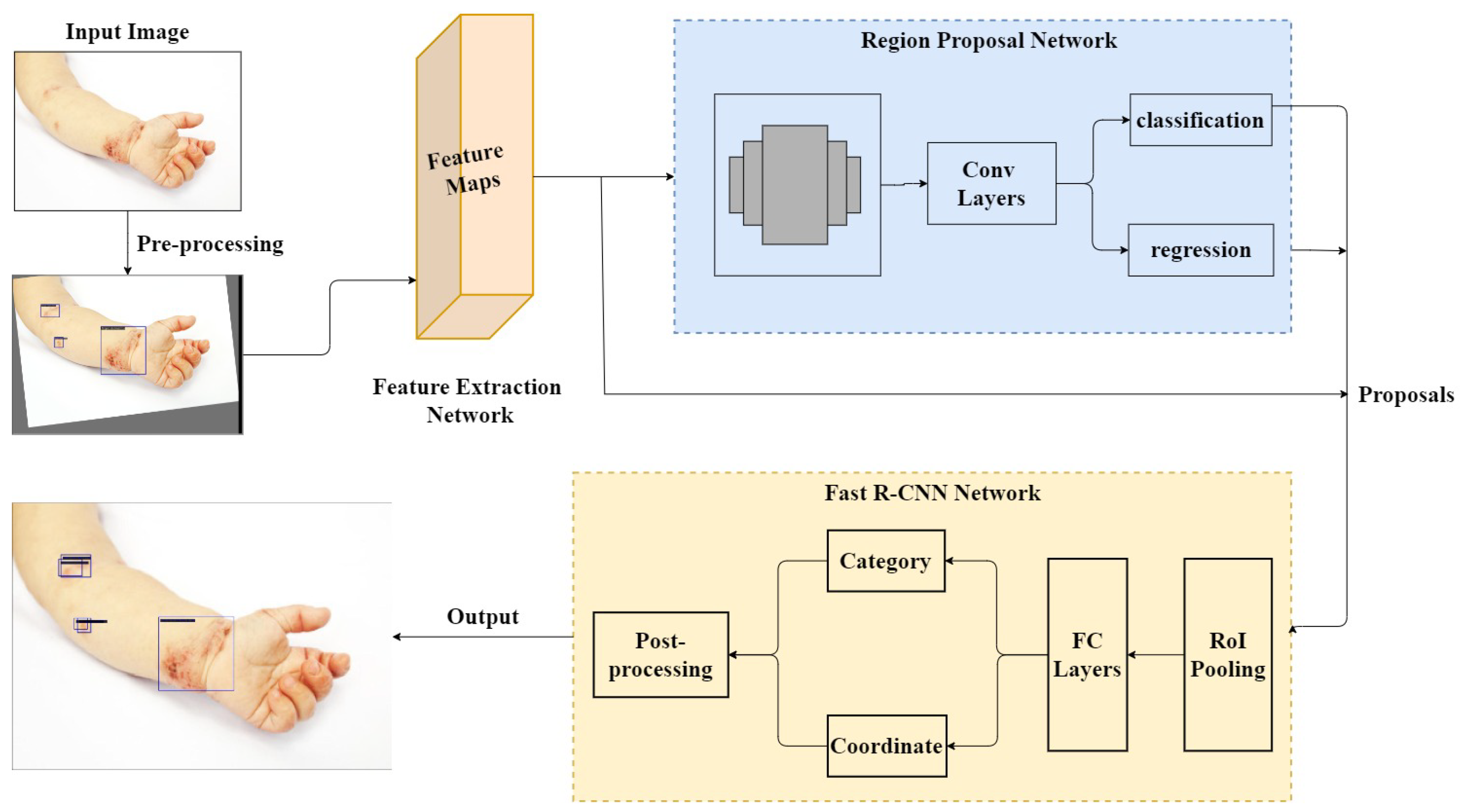
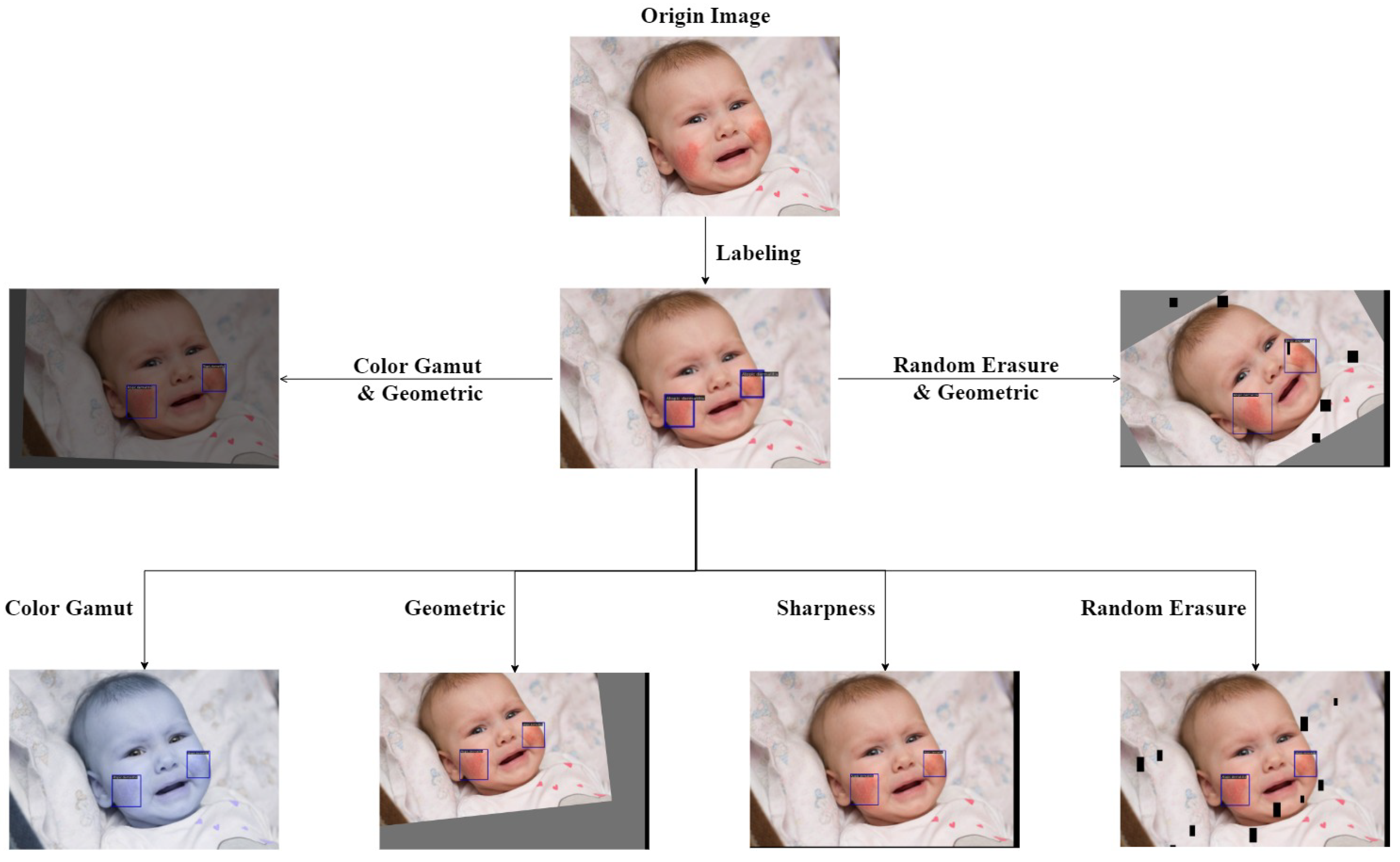
In this experiment, we use ResNet-50, ConvNeXt-T, Swin-T, Res2Net-101, ResNeXt-101, and PVTv2-B2, as the feature extraction networks, based on the Faster R-CNN algorithm. In training on the CPD-10 dataset, we observe varying degrees of overfitting and inadequate generalization ability. This is primarily due to the tiny data size. In this paper, we employ the Random Online Data Augmentation preprocessing method.

Table 6. Comparison of mAP for Random Online Data Augmentation, where $A{P}^S$ represents the AP for small objects with area $<{32}^2$, $A{P}^M$ represents the AP for medium objects with ${32}^2<$ area $<{96}^2$, and $A{P}^L$ represents the AP for large objects with area $>{96}^2$. All the results are the best of 5 runs.

Method	Backbone	mAP	${\mathit{AP}}^{\mathit{S}}$	${\mathit{AP}}^{\mathit{M}}$	${\mathit{AP}}^{\mathit{L}}$
Faster R-CNN	ResNet-50	0.485	0.458	0.439	0.499
	ResNet-50	0.522	0.413	0.499	0.529
	(RDA)	(+0.037)	(−0.045)	(+0.060)	(+0.030)
	ConvNeXt-T	0.521	0.414	0.475	0.526
	ConvNeXt-T	0.542	0.501	0.494	0.589
	(RDA)	(+0.021)	(+0.087)	(+0.019)	(+0.063)
	Swin-T	0.542	0.533	0.463	0.533
	Swin-T	0.566	0.488	0.490	0.534
	(RDA)	(+0.024)	(−0.045)	(+0.027)	(+0.001)
	Res2Net-101	0.465	0.441	0.406	0.457
	Res2Net-101	0.509	0.430	0.464	0.477
	(RDA)	(+0.044)	(−0.011)	(+0.058)	(+0.020)
	ResNeXt-101	0.497	0.345	0.428	0.520
	ResNeXt-101	0.534	0.428	0.494	0.540
	(RDA)	(+0.031)	(+0.083)	(+0.066)	(+0.020)
	PVTv2-B2	0.549	0.537	0.527	0.537
	PVTv2-B2	0.583	0.566	0.548	0.592
	(RDA)	(+0.034)	(+0.029)	(+0.021)	(+0.055)

displays a comparison of model mAP values, with RDA denoting the Random Online Data Augmentation method.

It is apparent that, in the classification and identification of natural images of common pediatric dermatoses, PVTv2-B2 has a superior feature extraction ability for disease representation in comparison to the convolutional networks ResNet-50, Res2Net-101, ResNeXt-101, and ConvNeXt-T, which possess local feature extraction ability, and the Swin-T network, which disregards the local feature continuity of the image. This is primarily due to the fact that the PVTv2-B2 backbone network is not only capable of extracting global information, but also contains more local continuity of the image, allowing it to effectively extract the overall characteristics of the disease representation. No matter which backbone network is used, however, there is overfitting in training due to the small scope of the dataset and the data’s homogeneity.

To address this issue, we employ the combined Random Online Augmentation method, which can improve the model’s mAP by more than $2\%$, with the AP of small, medium, and large objects all being improved to varying degrees. This is primarily because stochastic data augmentation can increase the diversity of training data, thereby alleviating the overfitting problem during training, making the model more robust and generalizable, and decreasing the leakage detection rate. However, the randomness of the data augmentation strategy causes instability in training. As shown in Table 6, although the overall performance of the model was improved after using the Random Online Data Augmentation method, the accuracy for small objects decreased instead with the ResNet-50, Swin-T, and Res2Net-101 networks, which may be because some small lesion representations are impacted by the stochastic augmentation strategy, e.g., chickenpox discrimination may be weakened under increasing illumination. To prove it, using ResNet-50 as the backbone network, we conducted repeated experiments with the Random Online Data Augmentation method, with RDA denoting the Random Online Data Augmentation method, the results of which are shown in

Table 7. Comparison of the accuracy of small objects with RDA. where $A{P}^S$ represents the AP for small objects with area $<{32}^2$, $A{P}^M$ represents the AP for medium objects with ${32}^2<$ area $<{96}^2$, and $A{P}^L$ represents the AP for large objects with area $>{96}^2$.

Method	Backbone	mAP	${\mathit{AP}}^{\mathit{S}}$	${\mathit{AP}}^{\mathit{M}}$	${\mathit{AP}}^{\mathit{L}}$
Faster R-CNN	ResNet-50	0.485	0.458	0.439	0.499
	ResNet-50 (RDA)	0.522	0.413	0.499	0.529
		0.527	0.434	0.508	0.535
		0.516	0.481	0.509	0.524

.

It can be seen from Table 7 that, while the overall performance of the model was improved in repeated experiments, small target detection accuracy enhancement was not stable, which is inextricably related to the randomness augmentation strategy, as well as the sensitivity of the network on small objects. In addition, although random online data enhancement improves the detection accuracy, the model’s precision is relatively low. This is due, in part, to the low resolution and subpar quality of the majority of the original images, which makes training difficult.

5.4.2. Selective Super-Resolution Reconstruction

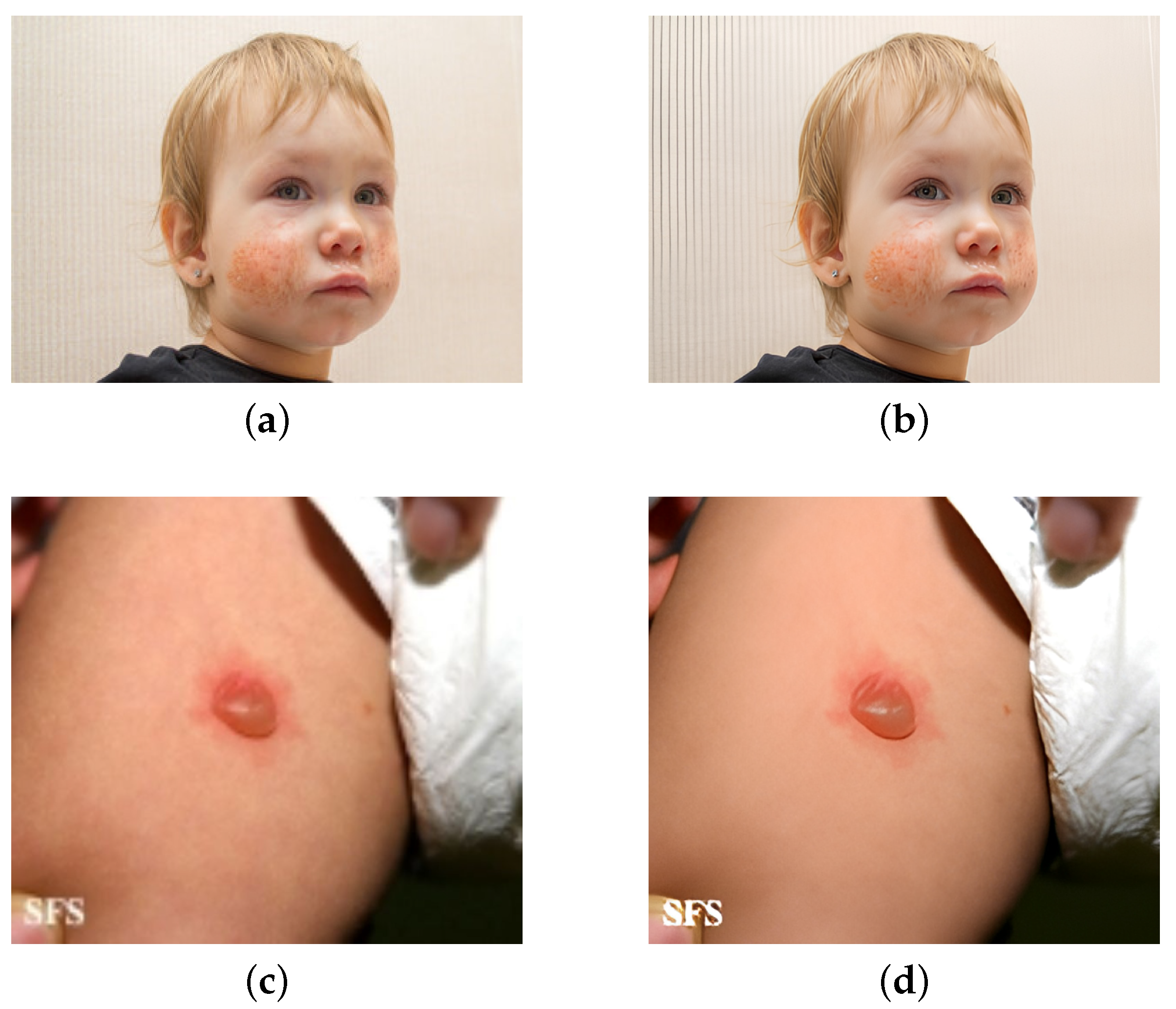
In order to increase the Precision of disease symptom recognition, it is important to address the hardware equipment limitations and other issues that result in fuzziness, poor quality, and insignificant interest regions. SwinIR was used to conduct super-resolution reconstruction on some low-quality original images that had been filtered-out based on the findings of Random Online Data Augmentation. The experimental results are shown in

Table 8. Comparison of experimental results with Selective Super-Resolution Reconstruction, RDA in the table represents Random Online Data Augmentation, and SSR represents Selective Super-Resolution Reconstruction. All the results are the best of 5 runs.

Method	Backbone	Pre-Processing	mAP
Faster R-CNN	ResNet-50	RDA	0.522
		RDA-SSR	0.535
			(+0.013)
	ConvNeXt-T	RDA	0.542
		RDA-SSR	0.558
			(+0.016)
	Swin-T	RDA	0.566
		RDA-SSR	0.580
			(+0.014)
	Res2Net-101	RDA	0.509
		RDA-SSR	0.536
			(+0.027)
	ResNeXt-101	RDA	0.534
		RDA-SSR	0.545
			(+0.011)
	PVTv2-B2	RDA	0.583
		RDA-SSR	0.602
			(+0.019)

.

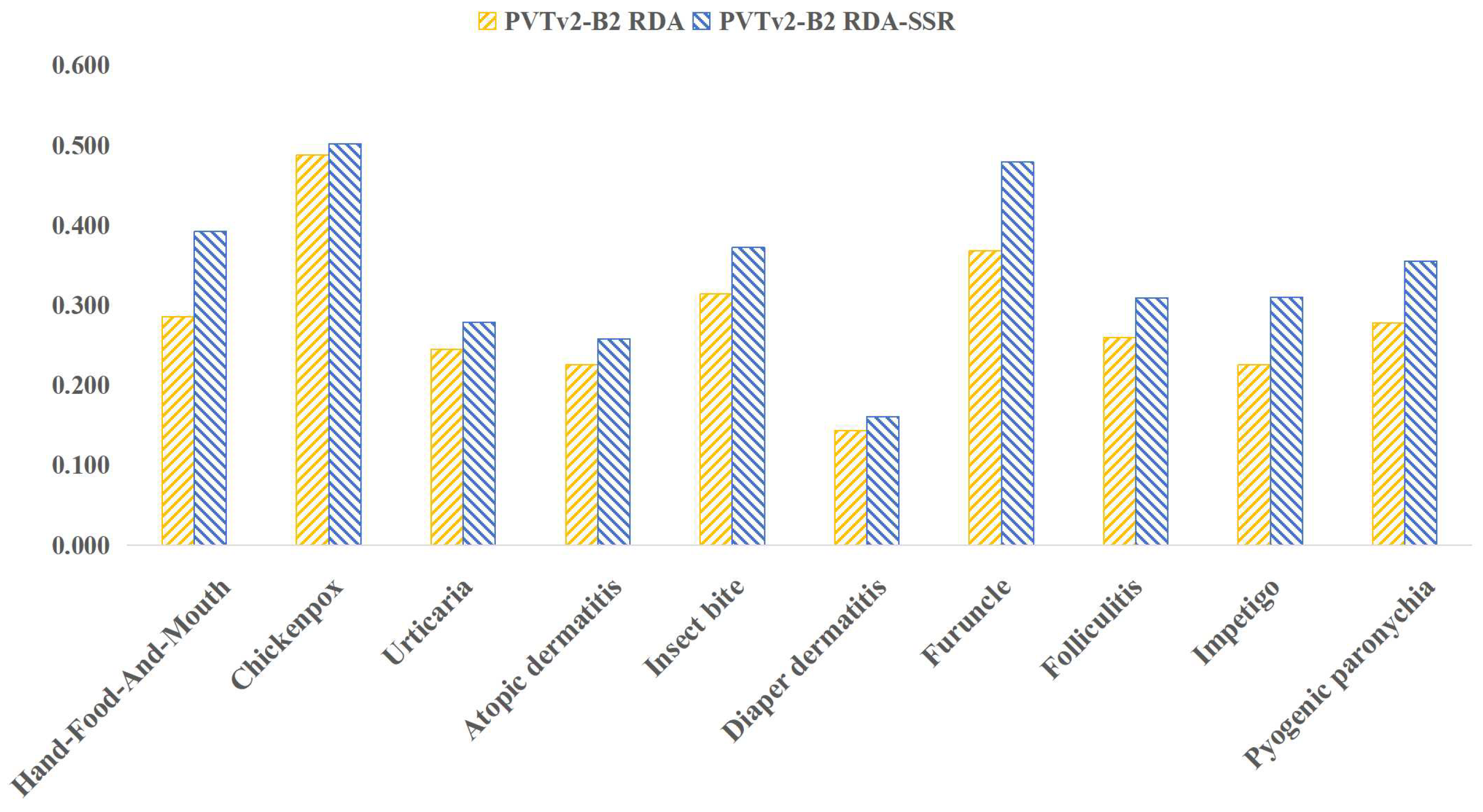
The experimental results demonstrate that using Super Resolution Reconstruction not only improves image quality, but also increases the accuracy of model detection and the mAP. The PVTv2-B2 feature extraction network, which achieves the greatest detection effect at present, was chosen to compare the precision of detecting 10 types of diseases. Figure 9 depicts the estimation of the effect of Selective Super Resolution Reconstruction.

It is evident that, after selective picture super-resolution reconstruction, the model’s disease detection accuracy increased. This is primarily due to the fact that, following image Super-Resolution Reconstruction, can more effectively enhance the clarity of the lesion area, sharpen the edge features, and reduce the impact of image noise, improving the accuracy of model detection.

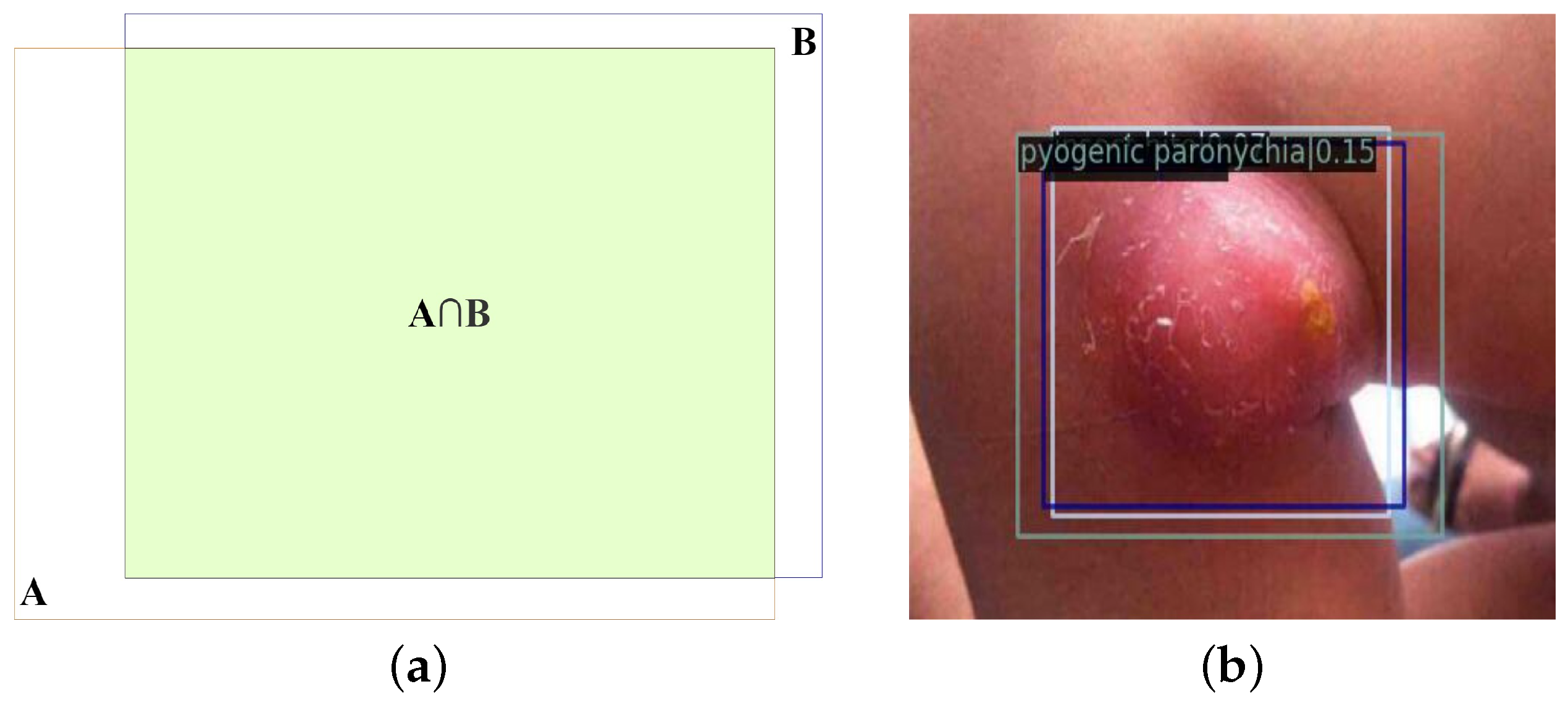
5.4.3. DK_Loss

There are 10 diseases involved in the CPD-10 dataset, and it has similarities and variations within each class that affect how challenging it is to diagnose different diseases. We developed the DK_Loss loss function to address this issue and enable the two-stage object recognition algorithm to concentrate more on the difficult-to-classify samples. We compare DK_Loss with the frequently used cross-entropy loss function in the two-stage object identification algorithm. The evaluation is conducted over the CPD-10 original dataset and the CPD-10 augmented dataset, which was created through online data augmentation and Selective Super-Resolution Reconstruction, respectively. When $k_{max}=1$, only the impact of the coefficients $1-q\left(x_t\right)$ is verified. Various values for $k_{max}$ are established and compared, and the optimal parameter values for $k_{max}$ are then determined. In

Table 9. Performance comparison over CPD-10 original dataset and augmented dataset based on different loss functions, where CPD-10 (RDA-SSR) represents the augmented dataset of CPD-10. All the results are the best of 5 runs.

Method	Loss Function	Backbone	Parameter	mAP
				CPD-10	CPD-10 (RDA-SSR)
Faster R-CNN	Cross-Entropy	ResNeXt-101	—	0.497	0.545
		Swin-T	—	0.542	0.580
		PVTv2-B2	—	0.549	0.602
	DK_Loss	ResNeXt-101	$k_{max}=1$	0.510 (+0.013)	0.551 (+0.006)
			$k_{max}=2$	0.512 (+0.015)	0.552 (+0.007)
			$k_{max}=3$	0.517 (+0.020)	0.554 (+0.009)
			$k_{max}=4$	0.521 (+0.024)	0.556 (+0.011)
		Swin-T	$k_{max}=1$	0.550 (+0.008)	0.585 (+0.005)
			$k_{max}=2$	0.553 (+0.011)	0.591 (+0.011)
			$k_{max}=3$	0.562 (+0.020)	0.590 (+0.010)
			$k_{max}=4$	0.560 (+0.018)	0.588 (+0.008)
		PVTv2-B2	$k_{max}=1$	0.562 (+0.013)	0.613 (+0.011)
			$k_{max}=2$	0.570 (+0.021)	0.619 (+0.017)
			$k_{max}=3$	0.576 (+0.027)	0.622 (+0.020)
			$k_{max}=4$	0.572 (+0.023)	0.617 (+0.015)
Cascade R-CNN	Cross-Entropy	Swin-T	—	0.538	0.577
		PVTv2-B2	—	0.549	0.590
	DK_Loss	Swin-T	$k_{max}=1$	0.545 (+0.007)	0.582 (+0.005)
			$k_{max}=2$	0.549 (+0.011)	0.583 (+0.006)
			$k_{max}=3$	0.551 (+0.013)	0.589 (+0.012)
			$k_{max}=4$	0.548 (+0.010)	0.581 (+0.004)
		PVTv2-B2	$k_{max}=1$	0.565 (+0.016)	0.599 (+0.009)
			$k_{max}=2$	0.568 (+0.019)	0.610 (+0.020)
			$k_{max}=3$	0.570 (+0.021)	0.605 (+0.015)
			$k_{max}=4$	0.557 (+0.008)	0.597 (+0.007)
Dynamic R-CNN	Cross-Entropy	ResNet-50	—	0.465	0.528
		PVTv2-B2	—	0.536	0.582
	DK_Loss	ResNet-50	$k_{max}=1$	0.471 (+0.006)	0.539 (+0.011)
			$k_{max}=2$	0.483 (+0.018)	0.540 (+0.012)
			$k_{max}=3$	0.485 (+0.020)	0.544 (+0.016)
			$k_{max}=4$	0.472 (+0.007)	0.531 (+0.003)
		PVTv2-B2	$k_{max}=1$	0.556 (+0.020)	0.594 (+0.012)
			$k_{max}=2$	0.563 (+0.027)	0.599 (+0.017)
			$k_{max}=3$	0.567 (+0.031)	0.604 (+0.022)
			$k_{max}=4$	0.558 (+0.022)	0.595 (+0.013)

, the testing findings are displayed.

Combining the experimental results of DK Loss on the original CPD-10 dataset and the augmented dataset in Table 9, we can observe that when $k_{max}=1$, i.e., only increasing the coefficient $1-q\left(x_t\right)$, the mAP of the model can be improved, which has a positive influence on training. This is because the corresponding score $q\left(x_t\right)$ of a sample’s true category can, to some extent, reflect the classification difficulty of a sample. The closer $q\left(x_t\right)$ is to 1, the more easily the sample can be considered a simple sample, and the closer the coefficient $1-q\left(x_t\right)$ is to 0, the easier the sample is. In contrast, the coefficient $q\left(x_t\right)$ is closer to 1 than to 0. By adding coefficients $1-q\left(x_t\right)$, the loss contribution of the samples that are simple to classify can be reduced, allowing the model to focus on the learning of samples that are difficult to classify.

Meanwhile, by varying $k_{max}$, we can also determine, for multiple detection boxes that can be identified as detecting the same lesion region, the predicted number of distinct categories $d{k}_t$, which play a complementary role to the coefficient $1-q\left(x_t\right)$. On the original CPD-10 dataset, the model mAP can be enhanced by more than 2%. When $k_{max}=2$ or $k_{max}=3$, i.e., $d{k}_t\in \{1,2,3\}$, it not only reduces the influence of anomalous samples within a certain range, but also improves the model’s mAP. By increasing the contribution of loss to hard samples, the model focuses on learning the majority of normal hard samples. In contrast, model training is degraded when $k_{max}=4$, i.e., $d{k}_t>3$, is influenced by the anomalous samples.

In addition, there is a significant disparity between the effect of model enhancement on the original CPD-10 dataset and the augmented dataset. When training on the CPD-10 original dataset, the PVTv2-B2 backbone network has the highest degree of overfitting and the most apparent improvement. This is primarily due to overfitting of varying degrees. It can be seen that the DK_Loss loss function not only addresses the problem of unbalanced hard and easy samples from the dataset, but also reduces overfitting during training, which is more pertinent to object detection on small datasets, for which data collection is more challenging.

Random Online Data Augmentation has a destabilizing effect on the experimental outcomes of the CPD-10 augmented dataset. To more accurately determine the value of $k_{max}$, we conduct experiments on the PASCAL VOC dataset, utilizing the VOC2007 training set, and evaluate the results on the VOC2007 test set. Additionally, we demonstrate the efficacy of the DK_Loss loss function.

As shown in

Table 10. Experimental results using ResNet-50-FPN backbone on PASCAL VOC2007 test set. All the results are the best of 5 runs.

Method	Cross-Entropy	DK_Loss
		${\mathit{k}}_{\mathit{max}}=\mathbf{1}$	${\mathit{k}}_{\mathit{max}}=\mathbf{2}$	${\mathit{k}}_{\mathit{max}}=\mathbf{3}$	${\mathit{k}}_{\mathit{max}}=\mathbf{4}$
Faster	0.775	0.783	0.787	0.789	0.787
R-CNN		(+0.008)	(+0.012)	(+0.014)	(+0.012)
Cascade	0.763	0.778	0.780	0.782	0.780
R-CNN		(+0.015)	(+0.017)	(+0.019)	(+0.017)
Dynamic	0.774	0.785	0.788	0.790	0.787
R-CNN		(+0.011)	(+0.014)	(+0.016)	(+0.013)

, when the parameter $k_{max}=3$ is set in the DK_Loss loss function, the mAP improves by $1.4\%$ for the Faster R-CNN, $1.9\%$ for the Cascade R-CNN, and $1.6\%$ for the Dynamic R-CNN, which is the current optimal, but taken as 4, the performance decreases instead, primarily because the DK_Loss loss function makes the model focus more on learning difficult samples, by increasing the loss contribution of difficult samples. If the value of $d{k}_t$ is not restricted with $k_{max}$, the focus of the model will always be on the abnormal hard-to-classify samples, which may not be correctly identified for other reasons, and mislead the subsequent optimization direction of the model. 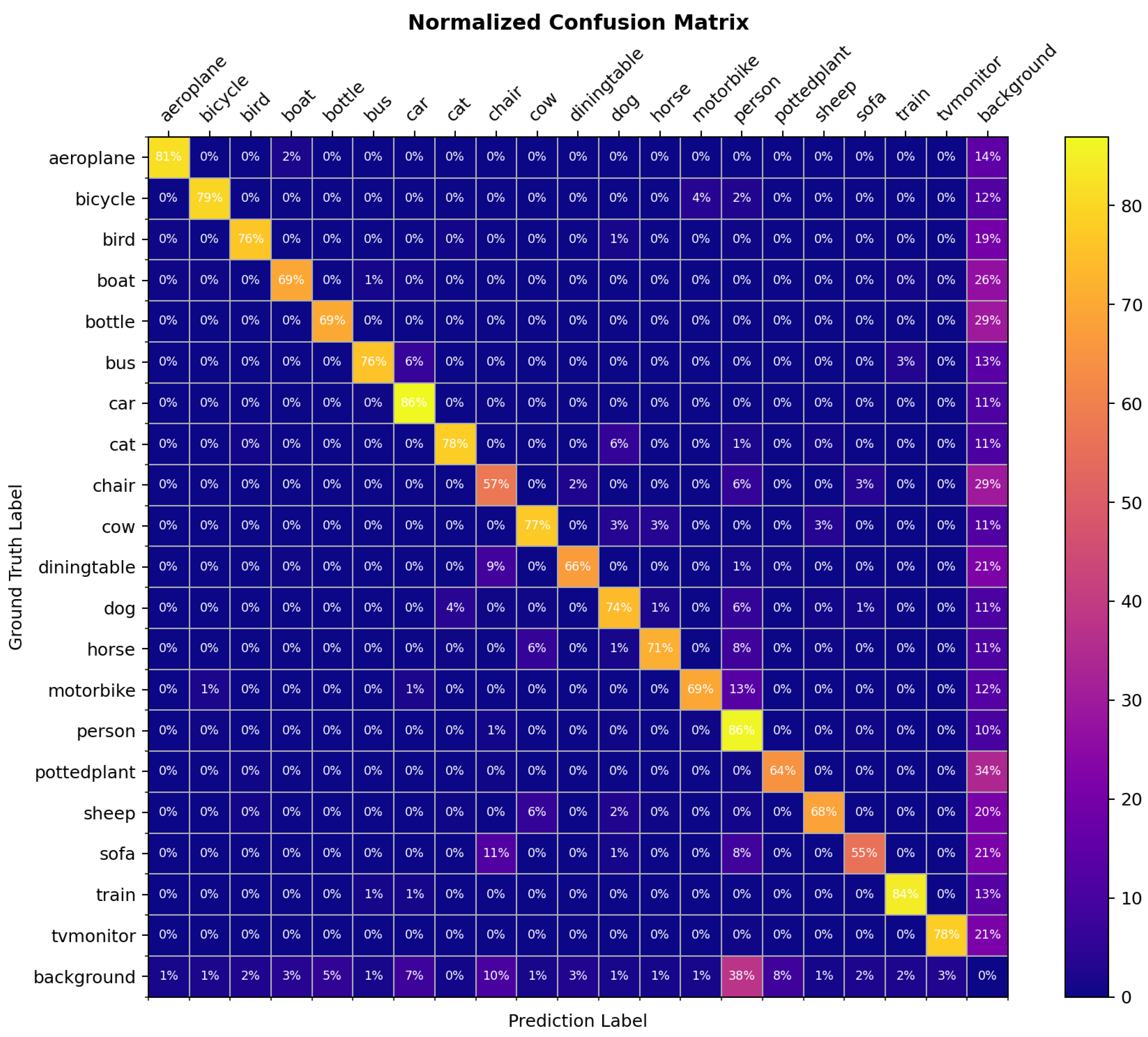Therefore, $k_{max}$ is not as large as possible, but depends on the number of misclassification categories of most normal samples in the dataset, making the model focus on the global situation of the distribution of normal difficult samples rather than extreme data. Additionally, the $k_{max}$’s value mainly depends on the likelihood of the misclassification category number for most samples. For example, for the PASCAL VOC2007 dataset, the confusion matrix of the model trained using the Cascade R-CNN is shown in Figure 10. It can be seen that most of the category confusion category numbers are less than or equal to 3, Consistent with the experimental results, so the proposed value of $k_{max}$ is set to 3.

The similarity between the conclusion and the CPD-10 dataset results validates the validity and generalizability of the DK_Loss loss function. Noting that the specific value of $k_{max}$ may vary across datasets, when $k_{max}$ is not applicable, you can observe the rough interval of $k_{max}$ value through the confusion matrix, based on the likelihood of the misclassification category number for most samples, and then experimentally set the optimal value.

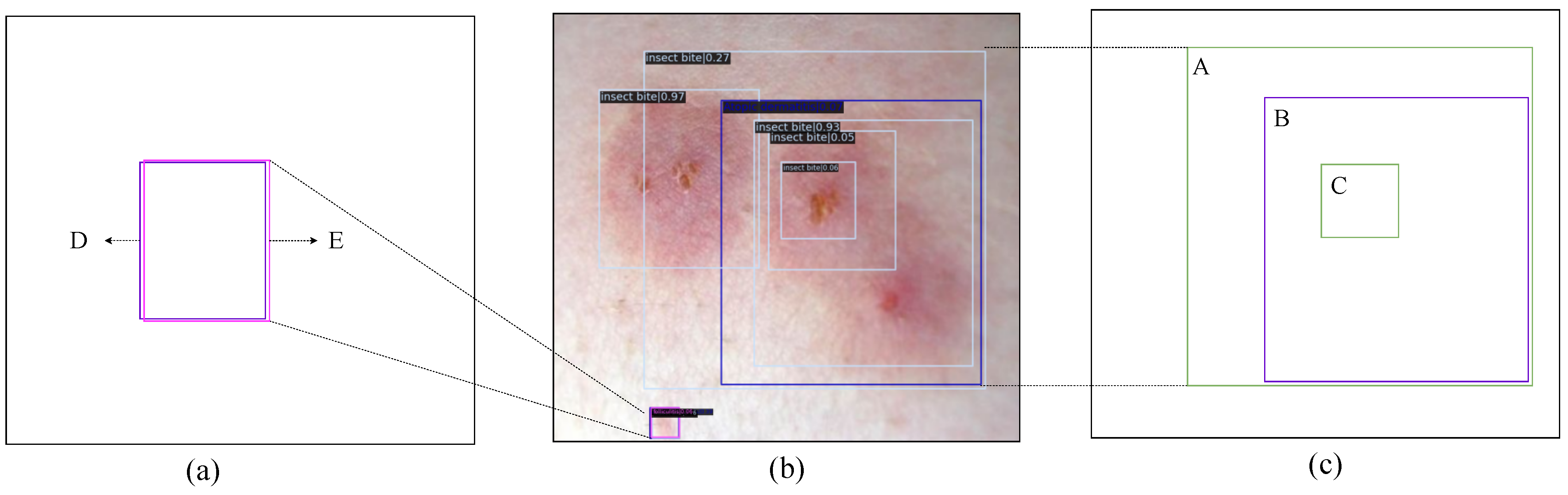
5.4.4. Fliter_nms

The experiments in this section are based on the outcomes of the DK_Loss experiments conducted in the previous section. The evaluation employs the PVTv2-B2 backbone network with different con_thr and cro_thr threshold parameters. First, eliminate the detection boxes for inclusion and contained relationships, and have distinct prediction categories and greater than con_thr confidence score differences. Then, the detection boxes that can be identified as detecting the same lesion region, have distinct prediction categories, and where the difference in confidence scores is greater than the set value cro_thr are deleted. The results of the experiments are presented in

Table 11. Comparison of adjustment results of different post-processing methods.

Method	Post-Processing	con_thr	cro_thr	mAP
Faster R-CNN	NMS	—	—	0.622
	Fliter_nms	0.70	—	0.620
		0.800	—	0.622
		0.90	—	0.622
		0.80	0.10	0.621
		0.80	0.20	0.621

.

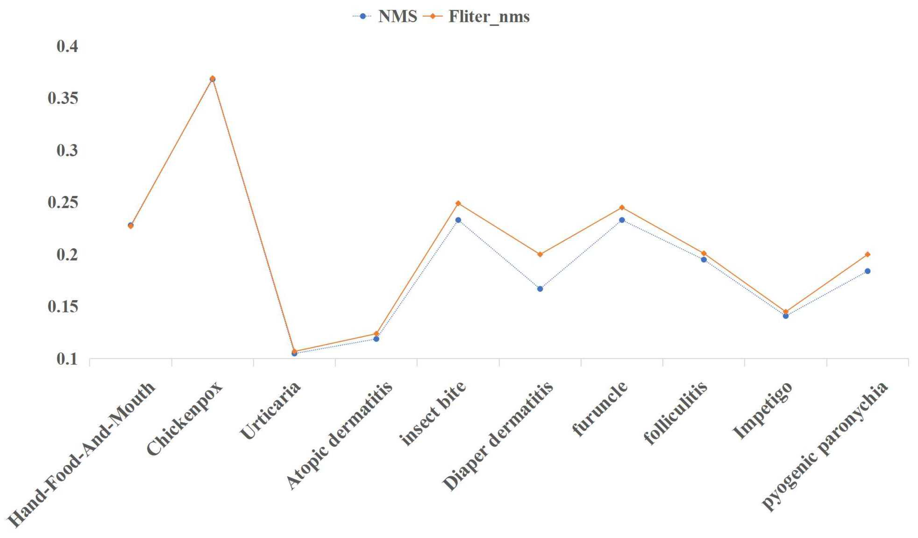
According to the experiment results, the mAP of the model with various con_thr and cro_thr threshold settings is relatively smooth. In addition, when $con\_thr=0.8$ and $cro\_thr=0.1$ are set, the best filtering effect is achieved for the misclassified boxes. Setting $con\_thr=0.8$ and $cro\_thr=0.1$ and utilizing various post-processing algorithms, Figure 11 compares the detection precision of 10 disease representations with $con\_thr=0.8$ and $cro\_thr=0.1$.

In Figure 11, it is clear that the Fliter_nms post-processing algorithm can increase accuracy while largely maintaining mAP. The Fliter_nms algorithm can reduce the interference caused by the messy detection boxes and satisfy the requirement of natural image object detection of common pediatric dermatoses, which takes precision as the first criterion, by filtering parts of the detection boxes that are obviously incorrect in prediction categories.

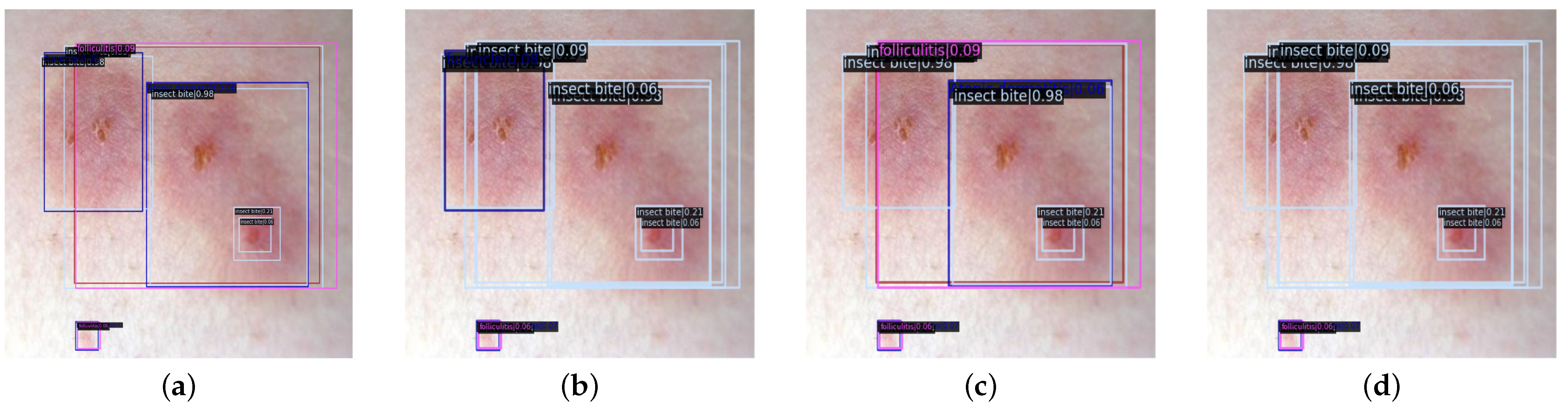
Simultaneously, we can observe an improvement in the precision of disease detection; however, compared to four diseases, namely insect bite, diaper dermatitis, furuncle, and pyogenic paronychia, there is no significant improvement. This is because of the fact that, for the screened detection boxes with evident prediction errors, the disease features in the prediction region cannot share a high degree of similarity with other disease features. Otherwise, it is highly probable that multiple prediction categories and their corresponding probabilities do not differ significantly, thereby failing to meet the threshold requirement. There are similarities between hand-foot-and-mouth disease, varicella, and folliculitis, as well as urticaria, atopic dermatitis, and impetigo, among the 10 diseases in the CPD-10 dataset. Consequently, the detection precision of these six diseases has not substantially improved. Real scenarios of natural images of common pediatric dermatoses after different post-processing methods are evaluated in Figure 12.

6. Conclusions

In this study, we create the clinical image dataset CPD-10 for common pediatric dermatologic diseases, which addresses the issues of a lack of image data, low resolution, unbalanced difficult and easy samples resulting from intra-class variability and inter-class similarity of disease representations, as well as the mixing of detection results, faced by the detection of common pediatric dermatologic diseases in natural scenes. In order to improve the expressiveness of the model, which focuses more on the learning of hard samples by increasing the loss contribution of hard samples within a certain range, we propose the DK_Loss loss function for the two-stage object detection algorithm. This algorithm is based on the two-stage object detection algorithm Faster R-CNN. To reduce the impact of false positive detection boxes and increase the accuracy of symptom representation detection, the Filter_nms post-processing method is proposed based on the NMS algorithm.

According to our extensive experiment results, we can draw the conclusion that object recognition can be significantly improved by using image pre-processing techniques such as Random Online Data Augmentation and Selective Image Super-resolution Reconstruction methods. Our loss function DK_Loss not only improves the model’s ability to learn from difficult samples, but it can also alleviate the overfitting issue, making it suitable for object detection on small datasets and significantly raising the mAP of detection. We also verified that the proposed Fliter_nms post-processing technique can reduce overlapping in the detection results and, additionally, increase precision.

References

1. Cartron, A.M.; Aldana, P.C.; Khachemoune, A. Pediatric teledermatology: A review of the literature. Pediatr. Dermatol. 2020, 38, 39–44. [Google Scholar] [CrossRef]
2. Ahmad, H.M.; Khan, M.J.; Yousaf, A.; Ghuffar, S.; Khurshid, K. Deep Learning: A Breakthrough in Medical Imaging. Curr. Med. Imaging 2020, 16, 946–956. [Google Scholar] [CrossRef]
3. Singh, C. Medical Imaging using Deep Learning Models. Eur. J. Eng. Technol. Res. 2021, 6, 156–167. [Google Scholar] [CrossRef]
4. Puttagunta, M.K.; Ravi, S. Medical image analysis based on deep learning approach. Multimed. Tools Appl. 2021, 80, 24365–24398. [Google Scholar] [CrossRef]
5. Rana, M.; Bhushan, M. Machine learning and deep learning approach for medical image analysis: Diagnosis to detection. Multimed. Tools Appl. 2022, 81, 1–39. [Google Scholar] [CrossRef] [PubMed]
6. Bhatt, C.; Kumar, I.; Vijayakumar, V.; Singh, K.U.; Kumar, A. The state of the art of deep learning models in medical science and their challenges. Multimed. Syst. 2021, 27, 599–613. [Google Scholar] [CrossRef]
7. Esteva, A.; Kuprel, B.; Novoa, R.A.; Ko, J.M.; Swetter, S.M.; Blau, H.M.; Thrun, S. Dermatologist-level classification of skin cancer with deep neural networks. Nature 2017, 542, 115–118. [Google Scholar] [CrossRef]
8. Li, H.; Pan, Y.; Zhao, J.; Zhang, L. Skin disease diagnosis with deep learning: A review. Neurocomputing 2021, 464, 364–393. [Google Scholar] [CrossRef]
9. Gessert, N.; Sentker, T.; Madesta, F.; Schmitz, R.; Kniep, H.C.; Baltruschat, I.M.; Werner, R.; Schlaefer, A. Skin Lesion Diagnosis using Ensembles, Unscaled Multi-Crop Evaluation and Loss Weighting. arXiv 2018, arXiv:1808.01694. [Google Scholar]
10. Zhang, J.; Xie, Y.; Xia, Y.; Shen, C. Attention Residual Learning for Skin Lesion Classification. IEEE Trans. Med. Imaging 2019, 38, 2092–2103. [Google Scholar] [CrossRef]
11. He, X.; He, X.; Wang, S.; Shi, S.; Tang, Z.; Wang, Y.; Zhao, Z.; Dai, J.; Ni, R.; Zhang, X.; et al. Computer-Aided Clinical Skin Disease Diagnosis Using CNN and Object Detection Models. In Proceedings of the 2019 IEEE International Conference on Big Data (Big Data), Los Angeles, CA, USA, 9–12 December 2019; pp. 4839–4844. [Google Scholar]
12. Xie, B.; He, X.; Zhao, S.; Li, Y.; Su, J.; Zhao, X.; Kuang, Y.; Wang, Y.; Chen, X. XiangyaDerm: A Clinical Image Dataset of Asian Race for Skin Disease Aided Diagnosis. In Proceedings of the LABELS/HAL-MICCAI/CuRIOUS@MICCAI, Shenzhen, China, 13–17 October 2019. [Google Scholar]
13. Udriștoiu, A.L.; Stanca, A.E.; Ghenea, A.E.; Vasile, C.M.; Popescu, M.; Udristoiu, S.; Iacob, A.V.; Castravete, Ș.C.; Gruionu, L.G.; Gruionu, G. Skin Diseases Classification Using Deep Leaning Methods. Curr. Health Sci. J. 2020, 46, 136–140. [Google Scholar] [PubMed]
14. He, K.; Zhang, X.; Ren, S.; Sun, J. Deep Residual Learning for Image Recognition. In Proceedings of the 2016 IEEE Conference on Computer Vision and Pattern Recognition (CVPR), Las Vegas, NV, USA, 27–30 June 2016; pp. 770–778. [Google Scholar]
15. Xie, S.; Girshick, R.B.; Dollár, P.; Tu, Z.; He, K. Aggregated Residual Transformations for Deep Neural Networks. In Proceedings of the 2017 IEEE Conference on Computer Vision and Pattern Recognition (CVPR), Honolulu, HI, USA, 21–26 July 2017; pp. 5987–5995. [Google Scholar]
16. Gao, S.; Cheng, M.M.; Zhao, K.; Zhang, X.; Yang, M.H.; Torr, P.H.S. Res2Net: A New Multi-Scale Backbone Architecture. IEEE Trans. Pattern Anal. Mach. Intell. 2019, 43, 652–662. [Google Scholar] [CrossRef]
17. Liu, Z.; Mao, H.; Wu, C.; Feichtenhofer, C.; Darrell, T.; Xie, S. A ConvNet for the 2020s. In Proceedings of the 2022 IEEE/CVF Conference on Computer Vision and Pattern Recognition (CVPR), New Orleans, LA, USA, 18–24 June 2022; pp. 11966–11976. [Google Scholar]
18. Liu, Z.; Lin, Y.; Cao, Y.; Hu, H.; Wei, Y.; Zhang, Z.; Lin, S.; Guo, B. Swin Transformer: Hierarchical Vision Transformer using Shifted Windows. In Proceedings of the 2021 IEEE/CVF International Conference on Computer Vision (ICCV), Montreal, QC, Canada, 10–17 October 2021; pp. 9992–10002. [Google Scholar]
19. Wang, W.; Xie, E.; Li, X.; Fan, D.P.; Song, K.; Liang, D.; Lu, T.; Luo, P.; Shao, L. PVTv2: Improved Baselines with Pyramid Vision Transformer. Comput. Vis. Media 2022, 8, 415–424. [Google Scholar] [CrossRef]
20. Hosang, J.H.; Benenson, R.; Schiele, B. Learning Non-maximum Suppression. In Proceedings of the 2017 IEEE Conference on Computer Vision and Pattern Recognition (CVPR), Honolulu, HI, USA, 21–26 July 2017; pp. 6469–6477. [Google Scholar]
21. Everingham, M.; Gool, L.V.; Williams, C.K.I.; Winn, J.M.; Zisserman, A. The Pascal Visual Object Classes (VOC) Challenge. Int. J. Comput. Vis. 2010, 88, 303–338. [Google Scholar] [CrossRef]
22. Cao, Y.; Wang, H. Object Detection: Algorithms and Prospects. In Proceedings of the 2022 International Conference on Data Analytics, Computing and Artificial Intelligence (ICDACAI), Zakopane, Poland, 15–16 August 2022; pp. 1–4. [Google Scholar]
23. Du, L.; Zhang, R.; Wang, X. Overview of two-stage object detection algorithms. J. Phys. Conf. Ser. 2020, 1544, 012033. [Google Scholar] [CrossRef]
24. Ge, Z.; Liu, S.; Wang, F.; Li, Z.; Sun, J. YOLOX: Exceeding YOLO Series in 2021. arXiv 2021, arXiv:2107.08430. [Google Scholar]
25. Law, H.; Deng, J. CornerNet: Detecting Objects as Paired Keypoints. Int. J. Comput. Vis. 2018, 128, 642–656. [Google Scholar] [CrossRef]
26. Girshick, R.B. Fast R-CNN. In Proceedings of the 2015 IEEE International Conference on Computer Vision (ICCV), Santiago, Chile, 7–13 December 2015; pp. 1440–1448. [Google Scholar]
27. Ren, S.; He, K.; Girshick, R.B.; Sun, J. Faster R-CNN: Towards Real-Time Object Detection with Region Proposal Networks. IEEE Trans. Pattern Anal. Mach. Intell. 2015, 39, 1137–1149. [Google Scholar] [CrossRef] [PubMed]
28. Cai, Z.; Vasconcelos, N. Cascade R-CNN: Delving Into High Quality Object Detection. In Proceedings of the 2018 IEEE/CVF Conference on Computer Vision and Pattern Recognition, Salt Lake City, UT, USA, 18–22 June 2018; pp. 6154–6162. [Google Scholar]
29. Zhang, H.; Chang, H.; Ma, B.; Wang, N.; Chen, X. Dynamic R-CNN: Towards High Quality Object Detection via Dynamic Training. In Computer Vision—ECCV 2020, Proceedings of the 16th European Conference, Glasgow, UK, 23–28 August 2020; Springer: Cham, Switzerland, 2020. [Google Scholar]
30. Shi, Z. Object Detection Algorithms: A Comparison. In Proceedings of the 2022 IEEE 4th International Conference on Civil Aviation Safety and Information Technology (ICCASIT), Dali, China, 12–14 October 2022; pp. 861–865. [Google Scholar]
31. Alomar, K.; Aysel, H.I.; Cai, X. Data Augmentation in Classification and Segmentation: A Survey and New Strategies. J. Imaging 2023, 9, 46. [Google Scholar] [CrossRef]
32. Yang, S.; Xiao, W.T.; Zhang, M.; Guo, S.; Zhao, J.; Furao, S. Image Data Augmentation for Deep Learning: A Survey. arXiv 2022, arXiv:2204.08610. [Google Scholar]
33. Raghavan, J.; Ahmadi, M. Data Augmentation Methods for Low Resolution Facial Images. In Proceedings of the TENCON 2022—2022 IEEE Region 10 Conference (TENCON), Hong Kong, China, 1–4 November 2022; pp. 1–6. [Google Scholar]
34. Lewy, D.; Ma’ndziuk, J. An overview of mixing augmentation methods and augmentation strategies. Artif. Intell. Rev. 2021, 56, 2111–2169. [Google Scholar] [CrossRef]
35. Dai, X.; Zhao, X.; Cen, F.; Zhu, F. Data Augmentation Using Mixup and Random Erasing. In Proceedings of the 2022 IEEE International Conference on Networking, Sensing and Control (ICNSC), Shanghai, China, 15–18 December 2022; pp. 1–6. [Google Scholar]
36. Devries, T.; Taylor, G.W. Improved Regularization of Convolutional Neural Networks with Cutout. arXiv 2017, arXiv:1708.04552. [Google Scholar]
37. Chen, P.; Liu, S.; Zhao, H.; Jia, J. GridMask Data Augmentation. arXiv 2020, arXiv:2001.04086. [Google Scholar]
38. Walawalkar, D.; Shen, Z.; Liu, Z.; Savvides, M. Attentive Cutmix: An Enhanced Data Augmentation Approach for Deep Learning Based Image Classification. In Proceedings of the ICASSP 2020—2020 IEEE International Conference on Acoustics, Speech and Signal Processing (ICASSP), Barcelona, Spain, 4–8 May 2020; pp. 3642–3646. [Google Scholar]
39. Hendrycks, D.; Mu, N.; Cubuk, E.D.; Zoph, B.; Gilmer, J.; Lakshminarayanan, B. AugMix: A Simple Data Processing Method to Improve Robustness and Uncertainty. arXiv 2019, arXiv:1912.02781. [Google Scholar]
40. Su, D.; Kong, H.; Qiao, Y.; Sukkarieh, S. Data augmentation for deep learning based semantic segmentation and crop-weed classification in agricultural robotics. Comput. Electron. Agric. 2021, 190, 106418. [Google Scholar] [CrossRef]
41. Goodfellow, I.; Pouget-Abadie, J.; Mirza, M.; Xu, B.; Warde-Farley, D.; Ozair, S.; Courville, A.; Bengio, Y. Generative Adversarial Networks. Commun. ACM 2020, 63, 139–144. [Google Scholar] [CrossRef]
42. Hiasa, Y.; Otake, Y.; Takao, M.; Matsuoka, T.; Takashima, K.; Prince, J.L.; Sugano, N.; Sato, Y. Cross-modality image synthesis from unpaired data using CycleGAN: Effects of gradient consistency loss and training data size. In Simulation and Synthesis in Medical Imaging, Proceedings of the Third International Workshop, SASHIMI 2018, Held in Conjunction with MICCAI 2018, Granada, Spain, 16 September 2018; Springer: Cham, Switzerland, 2018. [Google Scholar]
43. Cheng, M.; Wang, H.; Long, Y. Meta-Learning-Based Incremental Few-Shot Object Detection. IEEE Trans. Circuits Syst. Video Technol. 2022, 32, 2158–2169. [Google Scholar] [CrossRef]
44. Ganesh, A.H.; Xu, B. A review of reinforcement learning based energy management systems for electrified powertrains: Progress, challenge, and potential solution. Renew. Sustain. Energy Rev. 2022, 154, 111833. [Google Scholar] [CrossRef]
45. Bashir, S.M.A.; Wang, Y.; Khan, M.A. A comprehensive review of deep learning-based single image super-resolution. PeerJ Comput. Sci. 2021, 7, e621. [Google Scholar] [CrossRef]
46. Shukla, A.; Merugu, S.; Jain, K. A Technical Review on Image Super-Resolution Techniques. In Advances in Cybernetics, Cognition, and Machine Learning for Communication Technologies; Springer: Singapore, 2020. [Google Scholar]
47. Chen, H.; He, X.; Qing, L.; Wu, Y.; Ren, C.; Zhu, C. Real-World Single Image Super-Resolution: A Brief Review. Inf. Fusion 2021, 79, 124–145. [Google Scholar] [CrossRef]
48. Wang, X.; Yu, K.; Wu, S.; Gu, J.; Liu, Y.; Dong, C.; Loy, C.C.; Qiao, Y.; Tang, X. ESRGAN: Enhanced Super-Resolution Generative Adversarial Networks. In Proceedings of the ECCV Workshops, Munich, Germany, 8–14 September 2018. [Google Scholar]
49. Ji, X.; Cao, Y.; Tai, Y.; Wang, C.; Li, J.; Huang, F. Real-World Super-Resolution via Kernel Estimation and Noise Injection. In Proceedings of the 2020 IEEE/CVF Conference on Computer Vision and Pattern Recognition Workshops (CVPRW), Seattle, WA, USA, 14–19 June 2020; pp. 1914–1923. [Google Scholar]
50. Zhang, K.; Liang, J.; Gool, L.V.; Timofte, R. Designing a Practical Degradation Model for Deep Blind Image Super-Resolution. In Proceedings of the 2021 IEEE/CVF International Conference on Computer Vision (ICCV), Montreal, QC, Canada, 10–17 October 2021; pp. 4771–4780. [Google Scholar]
51. Wang, X.; Xie, L.; Dong, C.; Shan, Y. Real-ESRGAN: Training Real-World Blind Super-Resolution with Pure Synthetic Data. In Proceedings of the 2021 IEEE/CVF International Conference on Computer Vision Workshops (ICCVW), Montreal, BC, Canada, 11–17 October 2021; pp. 1905–1914. [Google Scholar]
52. Liang, J.; Cao, J.; Sun, G.; Zhang, K.; Gool, L.V.; Timofte, R. SwinIR: Image Restoration Using Swin Transformer. In Proceedings of the 2021 IEEE/CVF International Conference on Computer Vision Workshops (ICCVW), Montreal, BC, Canada, 11–17 October 2021; pp. 1833–1844. [Google Scholar]
53. Yeung, M.; Sala, E.; Schönlieb, C.B.; Rundo, L. Unified Focal loss: Generalising Dice and cross entropy-based losses to handle class imbalanced medical image segmentation. Comput. Med. Imaging Graph. 2021, 95, 102026. [Google Scholar] [CrossRef] [PubMed]
54. Jadon, S. A survey of loss functions for semantic segmentation. In Proceedings of the 2020 IEEE Conference on Computational Intelligence in Bioinformatics and Computational Biology (CIBCB), Viña del Mar, Chile, 27–29 October 2020; pp. 1–7. [Google Scholar]
55. Xie, S.; Tu, Z. Holistically-Nested Edge Detection. Int. J. Comput. Vis. 2015, 125, 3–18. [Google Scholar] [CrossRef]
56. Kim, I. Online Hard Example Mining for Training One-Stage Object Detectors. KIPS Trans. Softw. Data Eng. 2018, 7, 195–204. [Google Scholar]
57. Lin, T.Y.; Goyal, P.; Girshick, R.B.; He, K.; Dollár, P. Focal Loss for Dense Object Detection. IEEE Trans. Pattern Anal. Mach. Intell. 2017, 42, 318–327. [Google Scholar] [CrossRef] [PubMed]
Figure 1. Structure of the fundamental Faster R-CNN.
Applsci 13 05958 g001
Figure 2. Example of the result after data augmentation.
Applsci 13 05958 g002
Figure 3. Example of comparison with k times super-resolution and k times magnified. (a,c) are the original images after k-fold magnification. (b,d) are the reconstructed images of the original images after k-fold super-resolution.
Applsci 13 05958 g003
Figure 4. The overlap of the detection box A and B.
Applsci 13 05958 g004
Figure 5. In (a), if the ratio of the area of A B to the area of detection box B is more than 95 % , then detection box B is considered to detect the same object region as detection box A. (b) is an example of diversity detection results generated by multiple detection boxes that can be identified as detecting the same lesion region.
Applsci 13 05958 g005
Figure 6. Framework of DKFD algorithm.
Applsci 13 05958 g006
Figure 7. Flow of d k t calculation.
Applsci 13 05958 g007
Figure 8. The intermingling of detection results. (a,c) correspond to a part of the detection results in the realistic scenario (b), respectively. According to the determination criteria, detection box D and detection box E in (a) can be identified as detecting the same lesion region with different prediction results, while detection box B in (c) is contained by detection box A and also contains detection box C.
Applsci 13 05958 g008
Figure 9. Comparison of model detection precision.
Applsci 13 05958 g009
Figure 10. Confusion matrix using the Cascade R-CNN trained on PASCAL VOC2007.
Applsci 13 05958 g010
Figure 11. Compare the effect of different post-processing methods.
Applsci 13 05958 g011
Figure 12. Comparison of NMS and Fliter_nms post-processing methods. (a) is the effect of the NMS post-processing method; (b) is the effect of removing the detection box with the contained relationship; (c) is the effect of removing the detection box deemed to detect the same symptomatic region; (d) is the effect of the Fliter_nms post-processing method that combines the (b,c).
Applsci 13 05958 g012