Analysis of Numerical Micromodulus Coupled with Influence Function for Brittle Materials via Bond-Based Peridynamics

Abstract

In this paper, the numerical micromodulus is derived for the plane stress problem to develop a new insight into the application of bond-based peridynamics. Considering the nonlocal property of peridynamics, the numerical micromodulus coupled with influence function provides a reasonable description of the long-range force effect. Through several numerical applications, the effectiveness of the numerical modulus coupled with various influence functions to simulate deformation and failure is analyzed. In addition, a load increment algorithm based on fictitious density is developed specifically for quasi-static problems. It is indicated that the introduction of the influence function can enhance the accuracy in deformation and failure simulation, which is valuable for the advancement and application of numerical micromoduli. Through a comprehensive trade-off between simulation accuracy and stability, the numerical micromodulus coupled with the exponential influence function proves to be the more effective option for brittle material.

1. Introduction

Peridynamics (PD) is a nonlocal theory originally developed to address discontinuity issues [1], which discretizes an object into a number of material points connected by bonds. Different from conventional continuum mechanics (CCM), PD theory adopts the integral form of a governing equation without any spatial derivative [2]. The macroscopic cracking is strongly associated with spontaneously progressive breaking of bonds within the model [3]. Therefore, PD can predict damage development without additional assumptions as in the CCM, for example, crack extension criteria and node enrichment functions. PD provides a powerful tool to analyze material and structural failure processes [4,5], and has already been successfully applied to various problems, such as deformation and fracture simulation for brittle materials [6,7,8,9,10,11], asphalt [12], ferrite and pearlite wheel materials [13] and composite beams [14], etc.

Currently, generic variations of PD fall into two branches: bond-based peridynamics (BBPD) and state-based peridynamics (SBPD) [15]. The SBPD is a reformulation of the BBPD relations, which is divided into ordinary state-based PD and nonordinary state-based PD. The SBPD introduces the force vector state T, which maps the deformation state M to the force state T at all points within the affect region, and the bond force depends on the deformation of all bonds in the affected region. Nevertheless, the BBPD model is more simple to comprehend and carry out, which is well suited in multiscale analyses of composite materials, involving deformation and brittle fracture analysis [16,17,18,19,20,21,22]. The prototype microelastic brittle (PMB) model [23] is the most widely employed bond force constitutive model in BBPD, which is a linear microelastic model firstly proposed to simulate brittle failure process [24] in materials such as concrete [21,25,26,27,28,29] and cement [30,31]. The bond force in PMB can be regarded as the spring force, and the micromodulus represents the bond stiffness.

A micromodulus can be calculated based on both the energy equivalence principle and force intensity. For instance, Liu [32] developed the expression of the one-dimensional (1D) numerical micromodulus by introducing the concept of PD stress for linear elastic solids, which provides a new inspiration for the implementation of PD. However, there is a lack of research on the numerical micromodulus for the two-dimensional (2D) model. Some practical engineering problems (e.g., thin plate tension and compression) can be simplified into plane problems with the purpose of low computational expense and high precision. Therefore, it is necessary to address this knowledge gap. In this work, the numerical micromodulus for the 2D plane stress problem is explored first.

It is important to note that any numerical method will have errors. Technical aspects such as the loading algorithm and long-range force effect must be considered to achieve higher computational accuracy while minimizing expenses in BBPD. In practical application, the micromodulus is typically a constant when the interaction range is determined, that is, the bond force does not vary with the distance between two points [16]. As a matter of fact, it does not conform to the laws of physics due to the nonlocal feature in PD. Essentially, bond force owns the long-range force effect, which is similar to the atomic potential, that is, the bond force between two points decreases as their distance increases. The previous studies have revealed that long-range force effects can be represented by the influence function [33,34]. Therefore, in order to improve the applicability of the numerical micromodulus, it is necessary to introduce the influence function into the numerical micromodulus and explore the effect of the influence function types on the simulation precision.

To bridge the knowledge gaps mentioned above, the numerical micromodulus for the plane stress problem is derived first in the frame of BBPD. Subsequently, various types of influence functions are introduced into the numerical micromodulus. Additionally, to better solve the quasi-static problem, a load increment algorithm based on fictitious density is advanced. Several typical applications are investigated to explore the effect of different influence functions on the simulation accuracy. Through a comprehensive trade-off between simulation accuracy and stability, the more effective influence function is selected.

The flowchart for this paper is shown in Figure 1. Section 2 briefly reviews the theoretical foundation. Section 3 derives the numerical micromodulus and illustrates the influence function category. Numerical implementation and a novel loading algorithm are presented in Section 4. Numerical applications and discussion are claimed in Section 5. In the end, Section 6 sums up the conclusions obtained from this paper.

2. Theoretical Foundation

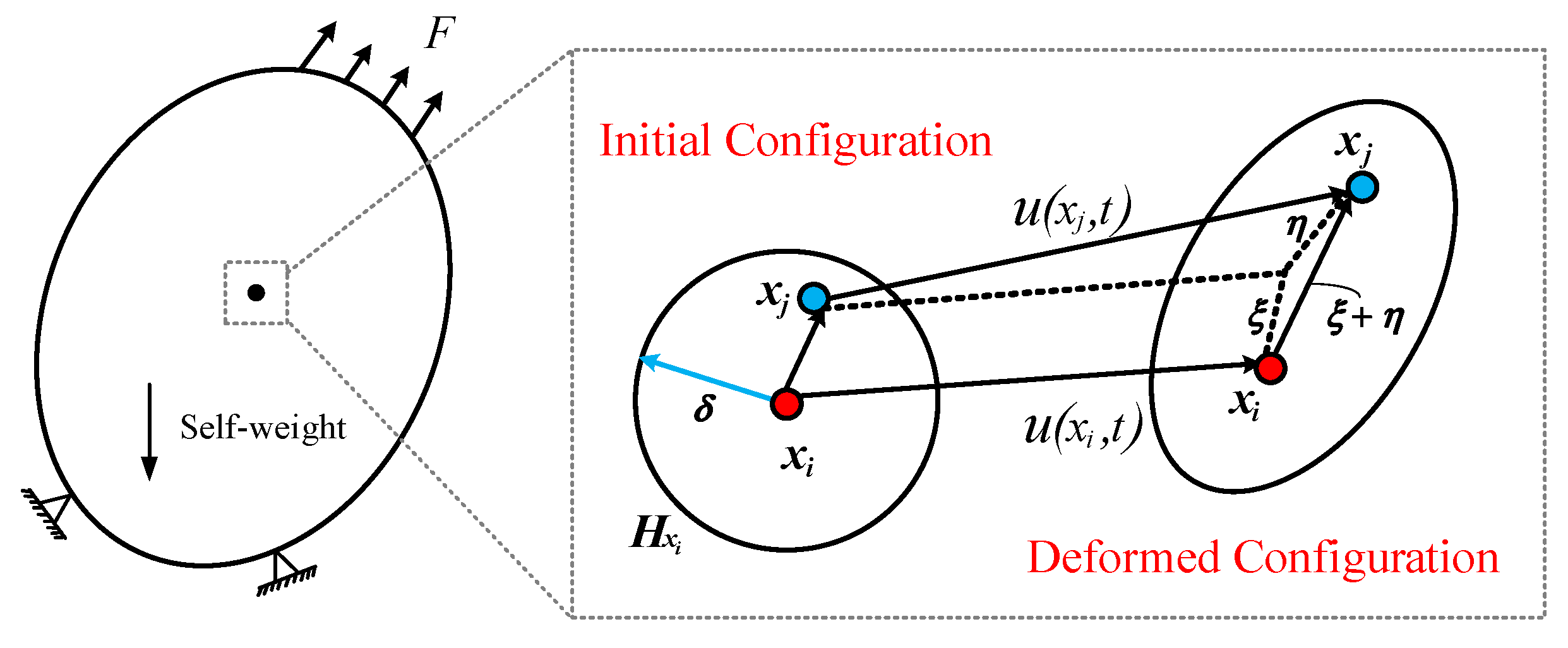
The PD governing formulation [1] is an integral form, which is effective at the discontinuity without facing any difficulties. In the BBPD frame, a material point $x_i$ interacts with other points $x_j$ in the horizon $H_{x_i}$ by bonds. The $\delta$ denotes the nonlocal range of point $x_i$, as depicted in Figure 2. The PD governing formulation of point $x_i$ at time t is written as illustrated,

$$\rho (x_i)\ddot{u}(x_i,t)={\displaystyle {\int }_{H_{x_i}}\mathbf{f}(x_i,x_j,u(x_i,t), }u(x_j,t),t)dV+b(x_i,t)$$

(1)

where $\ddot{u}$ is the acceleration and $\mathbf{f}$ designates the bond force constitutive function to describe the interaction on the point $x_i$ exerted by point $x_j$ in horizon $H_{x_i}$ at time t. $u$ and $dV$ represent the displacement and the volume of point $x_i$, respectively. b is the external loading density.

The relative position between the point $x_i$ and $x_j$ in $H_{x_i}$ is revealed as $\xi =x_j-x_i$. $\eta =u(x_j,t)-u(x_i,t)$ denotes the relative displacement at time t.

The bond force $\mathbf{f}$ remains zero beyond $H_{x_i}$, which is expressed as

$$\mathbf{f}(\eta ,\xi )=0 \forall \eta , if ‖ \xi ‖>\delta$$

(2)

The bond force function $\mathbf{f}$ has the following properties:

The bond force function $\mathbf{f}$ is derived from a potential $\omega$ for the microelastic material [1]

$$\mathbf{f}(\eta ,\xi )=\frac{\partial \omega }{\partial \eta }(\eta ,\xi )=\mathrm{f}(\eta ,\xi )\frac{\eta +\xi }{‖\eta +\xi ‖} \forall \eta ,\xi$$

(3)

in which $\mathrm{f}(\eta ,\xi )$ is a scalar-valued function and $\frac{\eta +\xi }{‖\eta +\xi ‖}$ denotes the direction vector of the bond after the movement of the points.

It satisfies the balance of linear momentum, as

$$-\mathbf{f}(\eta ,\xi )=\mathbf{f}(-\eta ,-\xi ) \forall \eta ,\xi$$

(4)

It satisfies the balance of angular momentum, as

$$(\eta +\xi )\times \mathbf{f}(\eta ,\xi )=0$$

(5)

The PMB model describes the microelastic material [24] in which the bond force function is obtained from a microelastic potential, expressed as

$$f(\eta ,\xi )=\frac{\partial \omega }{\partial \eta }(\eta ,\xi )=\frac{\partial (\frac{1}{2}c{s}^2\xi )}{\partial \eta }=cs\frac{\eta +\xi }{‖\eta +\xi ‖} \forall \eta ,\xi$$

(6)

where c denotes the micromodulus function representing the bond stiffness and the numerical micromodulus solved in this paper will be used here. $s=(\left|\eta +\xi \right|-\left|\xi \right|)/\left|\xi \right|$ reveals the elongation of a bond.

The damage at point $x_i$ is expressed in Equation (7)

$$D(x_i,t)=1-\frac{{\displaystyle {\int }_{H_{x_i}}\mu (x_i,t)dV}}{{\displaystyle {\int }_{H_{x_i}}dV}}$$

(7)

in which $\mu (x_i,t)$ represents the damage function of a bond,

$$\mu (x_i,t)=\left\{\begin{array}{l}1 s<s_0\\ 0 else\end{array}\right.$$

(8)

where $s_0$ denotes the critical elongation, which will be obtained according to fracture energy [24] or fracture strength [35,36].

3. Numerical Micromodulus

According to the 1D numerical micromodulus proposed in the literature [32], the numerical micromodulus for the plane stress problem is derived in this section. Firstly, the 1D numerical micromodulus is briefly reviewed [32]. Then, the 2D numerical micromodulus is developed by considering the PD stress and Hooke’s law of linear elasticity. Finally, the influence functions which denote the spatial intensity distribution of the long-range force are introduced into the numerical micromodulus.

3.1. One-Dimensional Numerical Micromodulus

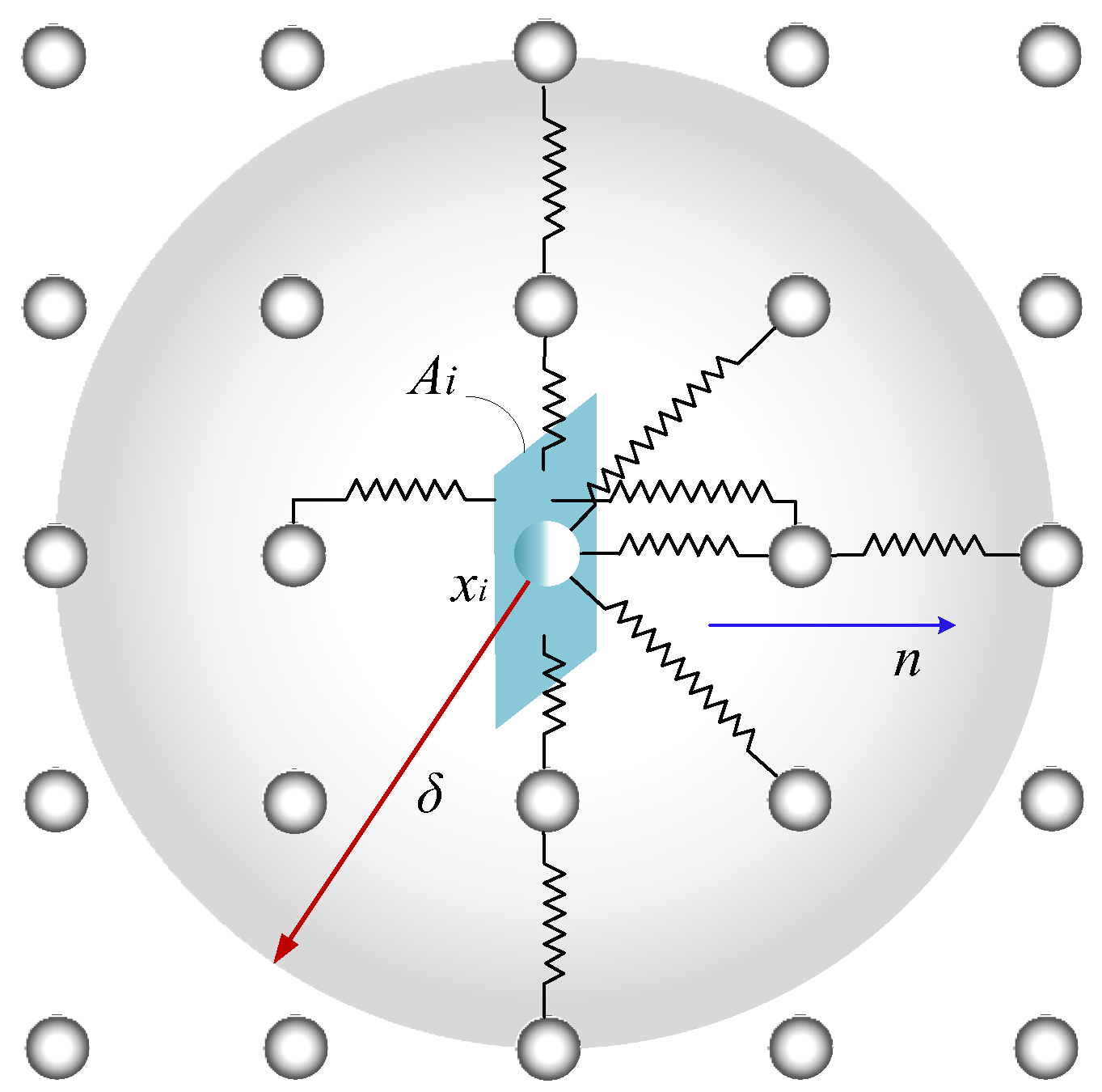
Consider a bar subjected to tension load, the spacing between material points is $\Delta x$. The volume of the material point is ${(\Delta x)}^3$. In the PMB model, bond force is considered as spring force. When $\delta =2\Delta x$, a set of bonds can pass through or end in the cross-section $A_i$ of point $X_i$ from a positive direction, as illustrated in Figure 3. The total bond force per unit volume acting through $A_i$ is written as Equation (9),

$$f_V^L={\displaystyle \sum _{j=1}^{k}f(\eta ,\xi )V_j}=2f{V}_j=2c_{1}s{V}_j$$

(9)

in which k is the number of bonds and $c_1$ is the numerical micromodulus of the 1D model.

Thus, the resultant force is

$$F=2c_{1}s{V}_j{V}_i$$

(10)

Then, the PD stress ${\sigma }_x$ at $X_i$ is

$${\sigma }_x=F/A_i=2c_{1}s\Delta x^4$$

(11)

According to Hooke’s law, the peridynamic elasticity modulus $E_{PD}$ can be given as

$$E_{PD}=\frac{{\sigma }_x}{s}=2c_1\Delta x^4$$

(12)

Since the elastic modulus is an inherent property of the material, $E_{PD}$ equals to the elasticity modulus $E$ in isotropic material; the $c_1$ in $\delta =2\Delta x$ is obtained as

$$c_1=\frac{E}{2\Delta x^4}$$

(13)

Similarly, $c_1$ for different horizons are listed in

Table 1. Numerical micromodulus $c_1$.

$\mathbf{Horizon} \mathit{\delta }$	$\mathbf{Numerical} \mathbf{Micromodulus} {\mathit{c}}_1$
2Δx	$\frac{E}{2\Delta x^4}$
3Δx	$\frac{2E}{9\Delta x^4}$
4Δx	$\frac{E}{8\Delta x^4}$
5Δx	$\frac{2E}{25\Delta x^4}$

.

3.2. Two-Dimensional Numerical Micromodulus

Assume a 2D isotropic plate with unit thickness, the bond elongation is a constant s under uniform deformation. E is the elastic modulus. The plate is discretized into N material points spaced $\Delta x$ apart and the horizon’s radius is $\delta =m\Delta x, (m=2,3,4,5)$. As demonstrated in Figure 4 for $\delta =2\Delta x$, the cross-section $A_i$ of point $x_i$ has several bonds in the positive direction passing through or ending at it. The numerical micromodulus denotes $c_2$.

The projection of a single bond force in the x-direction can be expressed in Equation (14)

$$f_x=f\frac{\left|x_j-x_i\right|}{‖\xi ‖}$$

(14)

in which $\left|x_j-x_i\right|$ is the x-distance for point $x_i$, $x_j$ and $f=c_{2}s$. It is a remarkable fact that f is reduced to 1/2 when the horizon $H_{x_i}$ contains half the $d{V}_j$, and f is reduced to 4/5 if the horizon $H_{x_i}$ contains four fifths $d{V}_j$. The PD stress ${\sigma }_x$ for the point $x_i$ can be expressed as

$${\sigma }_x=\frac{1}{A_i}{\displaystyle \sum _{j=1}^{N_M}(f_x{V}_j)V_i}$$

(15)

where $N_M$ is the number of bonds.

The definition of bond elongation is similar to the concept of strain ${\epsilon }_k { }_{(k=x,y)}$ in CCM. Thus, $s={\epsilon }_k { }_{(k=x,y)}$ and the PD stress ${\sigma }_x={\sigma }_y$ due to the isotropic expansion. The relationship between the PD stress and the bond elongation, s, can be rewritten as Equation (16) by using Hooke’s law of linear elasticity.

$$E=\frac{{\sigma }_x}{s}-\frac{\nu {\sigma }_y}{s}$$

(16)

It is worth noting that the BBPD restricted to a material with a fixed Poisson’s ratio ($\mathit{v}=1/3$ for the plane stress problem). Thus, the numerical micromodulus $c_2$ can be calculated by substituting $\mathit{v}=1/3$, Equations (14)–(16), which are illustrated in

Table 2. Numerical micromodulus $c_2$.

$\mathbf{Horizon} \mathit{\delta }$	$\mathbf{Numerical} \mathbf{Micromodulus} {\mathit{c}}_2$
2Δx	$0.405186768\frac{E}{\Delta x^4}$
3Δx	$0.108285522\frac{E}{\Delta x^4}$
4Δx	$0.047962844\frac{E}{\Delta x^4}$
5Δx	$0.025026356\frac{E}{\Delta x^4}$

for different horizon radii.

In summary, a preliminary exploration of numerical micromoduli $c_2$ is carried out based on the isotropic deformation. The great significance lies in addressing the existing research gap and providing a new insight for the numerical method application of PD. Further research, such as in the nonuniform deformation condition, will be needed in future.

3.3. Influence Function

The long-range force effect can be characterized by the influence function [16]. In order to improve the applicability of numerical micromodulus $c_2$, the influence function introduced into $c_2$ can be expressed in Equation (17).

$$c=c_{2}g(\xi ,\delta )$$

(17)

where $g(\xi ,\delta )$ is the influence function, which should hold the following requirements [22]:

$$\left\{\begin{array}{l}g(\xi ,\delta )\ge 0\\ \underset{\xi \to 0}{\lim }g(\xi ,\delta )=\max g\\ \underset{\xi \to \delta }{\lim }g(\xi ,\delta )=0\\ g(\xi ,\delta )=g(-\xi ,\delta )\\ {\displaystyle {\int }_{-\infty }^{\infty }\underset{\delta \to 0}{\lim }} g(\xi ,\delta )={\displaystyle {\int }_{-\infty }^{\infty }\Delta (\xi )dx=1}\end{array}\right.$$

(18)

in which $\Delta (\xi )$ is the Dirac delta function. $g(\xi ,\delta )=1$ means that the bond force is constant and will not change with the bond length. Eight types of influence functions published in previous studies are listed in

Table 3. Eight types of influence functions.

Type	$\mathit{g}(\mathit{\xi },\mathit{\delta })$	Symbol
Constant [24,37]	1	$g_1$
Exponential [38]	$e^{-\frac{\xi }{\delta }}$	$g_2$
Gaussian [39]	$e^{-(\frac{\xi }{\delta }{)}^2}$	$g_3$
Semi-elliptical [38]	$1-(\frac{\xi }{\delta }{)}^2$	$g_4$
Quartic polynomial [33]	$1-(\frac{\xi }{\delta }{)}^4$	$g_5$
Parabolic [16]	${(1-(\frac{\xi }{\delta }{)}^2)}^2$	$g_6$
Sixth-order polynomial [26]	${(1-(\frac{\xi }{\delta }{)}^2)}^3$	$g_7$
Cosine [26]	$\cos (\frac{\pi \xi }{2\delta })$	$g_8$

. For convenience, each influence function has a symbol, $g_i , i=1,2,3\dots 8$, which will be used in the follow-up paper.

As can be depicted from Table 3, these influence functions are based on physical parameters ($\delta$ and $\xi$), effectively expressing the physical properties of long-range force. Moreover, the spatial strength for the long-range force depends on the bond length. Except for $g_1$, the rest reflect the gradual weakening of the long-range force spatial strength distribution as the bond length increases.

4. Numerical Implementation

4.1. Discretization and Computation Processes

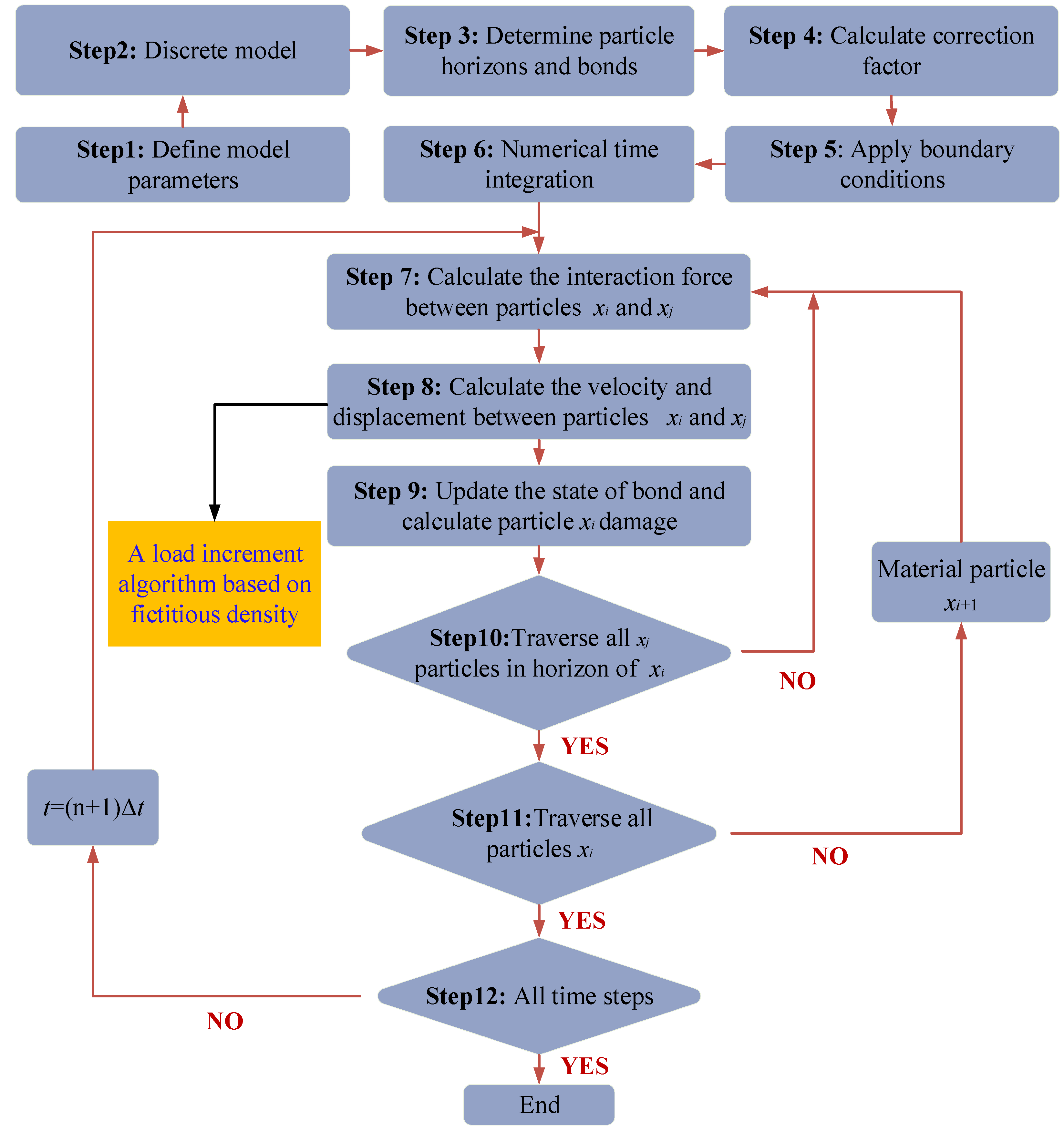
In this work, numerical implementation is realized in Matlab using self-compiled PD code, which can be simply described in the flow chart (seen Figure 5). The processes can be mainly divided into two parts: discretization and computation.

The discretization process starts with discretizing the object into material points with the uniform spacing, $\Delta x$, and the governing equation in integral form (Equation (1)) can be converted into a finite sum form, as re-expressed as

$$\begin{array}{ll}{\rho }_i{\ddot{u}}_i{}^n& ={\displaystyle \sum _{j=1}^{p}f(u_j{}^n-u_i{}^n,x_i-x_j)\Delta \overline{v}{V}_{ij}+b_i{}^n(x_i,t) }\\ & ={\displaystyle \sum _{j=1}^{p}f({\eta }_{ij}{}^n,{\xi }_{ij})\Delta \overline{v}{V}_{ij}+b_i{}^n(x_i,t) \forall x_j\in H_{x_i}}\end{array}$$

(19)

in which n represents the n-th time step, $p$ denotes the amount of points in $H_{x_i}$, $u_i{}^n=u(x_i,t=n\Delta t)$ and $b_i{}^n(x_i,t)$ stands for volume force density due to external load. $\Delta \overline{v}{V}_{ij}$ designates the effective computational volume of $x_j$ in $H_{x_i}$ and $\Delta \overline{v}$ is the volume correction factor as expressed in Equation (20).

$$\Delta \overline{v}=\left\{\begin{array}{l} 1 ‖\xi +\eta ‖\le \delta -\frac{\Delta x}{2}\\ (\frac{\delta -‖\xi +\eta ‖}{\Delta x}+\frac{1}{2}) \delta -\frac{\Delta x}{2}<‖\xi +\eta ‖\le \delta \\ 0 else\end{array}\right.$$

(20)

The computation process is the core part, which is accomplished by time step integration. The bond force and elongation are gained from calculating the displacement and velocity of points, so as to analyze the state of bonds and the point damage in each time step. For quasi-static problems, a load increment algorithm based on fictitious density is proposed (seen Step 8), which will be described in detail in Section 4.2.

4.2. A Load Increment Algorithm Based on Fictitious Density

The governing equation in motion form cannot be directly applied to quasi-static problems. Rather, substitute the artificial damping coefficient into Equation (1), which can be expressed as Equation (21).

$$\rho \ddot{u}+C\dot{u}=L+b$$

(21)

where C represents the artificial damping coefficient.

Previous studies often report that boundary particles may break prematurely when the model boundary is subjected to external load. Hence, the boundary region is usually designated as a nonfailure region to prevent the boundary material points from tearing apart from the model [16]. However, this is obviously not in accordance with the laws of physics, which limits the application of PD in quasi-static analysis to some extent.

Based on the concept of load increment proposed by Huang [16], a load increment algorithm based on fictitious density is proposed to solve this problem. The fictitious density, M, in the adaptive dynamic relaxation (ADR) scheme [40] has the ability to improve convergence and maintain the calculation stability. The purpose of setting the fictitious density is to accelerate the convergence by setting different virtual densities for each material point so that they have the same convergence time step. The algorithm is divided into the following steps:

(i)

The external load is gradually applied to the object in increments. The load increment is calculated in Equation (22).

$$\Delta \lambda =0.8\times \frac{2Ms\Delta x}{\Delta t^2\mathit{b}}, M=\frac{1}{4}\Delta t^2{\displaystyle \sum _{j=1}^p\left|K_{ij}\right|}$$

(22)

in which 0.8 is a safety factor. M is fictitious density [40], $K_{ij}$ is the stiffness matrix and $p$ is the amount of points in $H_{x_i}$.$\Delta t$ is the time step, which must satisfy the stability condition [24].

(ii)

The time step integral describes how points move in space and interact with their horizon points. The velocity and displacement of points are obtained by employing the central difference formula combined with the damping relaxation method, seen in Equation (23).

$$\left\{\begin{array}{l}\ddot{\mathit{u}}=(\frac{{\dot{\mathit{u}}}^{n+1/2}-{\dot{\mathit{u}}}^n}{1/2\Delta t}+\frac{{\dot{\mathit{u}}}^n-{\dot{\mathit{u}}}^{n-1/2}}{1/2\Delta t})/2=\frac{{\dot{\mathit{u}}}^{n+1/2}-{\dot{\mathit{u}}}^{n-1/2}}{\Delta t}\\ {\dot{\mathit{u}}}^{n+1/2}=\frac{{\dot{\mathit{u}}}^{n-1/2}}{1+C\Delta t/M}+\frac{(\mathit{L}+\mathit{b})}{C+M/\Delta t}\end{array}\right.$$

(23)

(iii)

After numerical iteration, the model would come to equilibrium when the convergence criterion is reached, which indicates that the next time step and load increment can be practiced in simulation. The convergence criterion is

$$\frac{{\displaystyle \sum _{i=1}^{N}R{E}_x}+{\displaystyle \sum _{i=1}^{N}R{E}_y}}{N}\le \gamma$$

(24)

where N stands for total number of material points. $R{E}_{x/y}$ represents relative error of displacement between the current iteration and the last iteration. $\gamma$ is a given convergence index.

5. Numerical Applications and Discussion

To validate the unique abilities of the proposed method in addressing deformation and failure, several numerical applications are conducted in this section. The time step $\Delta t={10}^{-6}\mathrm{s}$ satisfies the stability requirement. $C=5\times {10}^5 \mathrm{k}\mathrm{g}/{\mathrm{m}}^3\mathrm{s}$, $\gamma =0.005$ for quasi-static problems based on the convergence analysis.

5.1. Benchmark

In this subsection, the rationality of the self-compiled PD codes is verified through a benchmark without considering the influence function. The model results will be in contrast with the finite element (FEM) results.

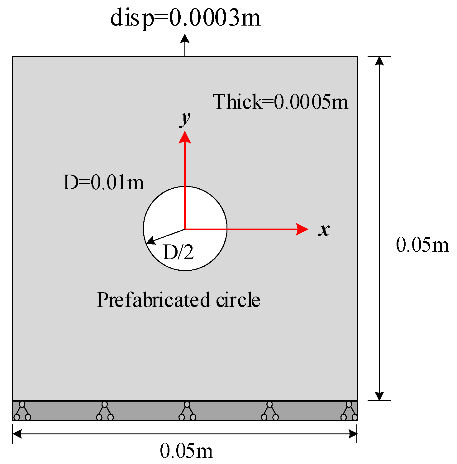
As displayed in Figure 6, there is a prefabricated circular hole with diameter of 0.01 m in the center of an isotropic plate. The bottom of the plate is fixed, and the top is subjected to 0.0003 m displacement load along the y direction. Material properties and PD model parameters are listed in

Table 4. Material properties and PD model parameters.

E(GPa)	v	$\mathit{\rho }$ (kg/m3)	$\mathsf{\Delta }\mathit{x}$ (m)	$\mathit{\delta }$ (m)	Influence Function
192	1/3	8000	0.0005	$2\Delta x,3\Delta x,4\Delta x,5\Delta x$	$g_1$

.

To explore the effect of horizon radius ($\delta$) on calculation accuracy, two column points along the x-axis and y-axis are selected, as depicted in Figure 7. The horizon radius has a certain impact on the computational precision of the PD model, and the calculation cost increases with the increase in horizon radius. The reason is that the horizon needs to contain a certain number of material points due to nonlocal characteristics. Moreover, the result is also related to the convergence of the PD model. In this model, the PD solutions are in good agreement with the FEM solutions when the horizon radius is equal to or greater than $3\Delta x$.

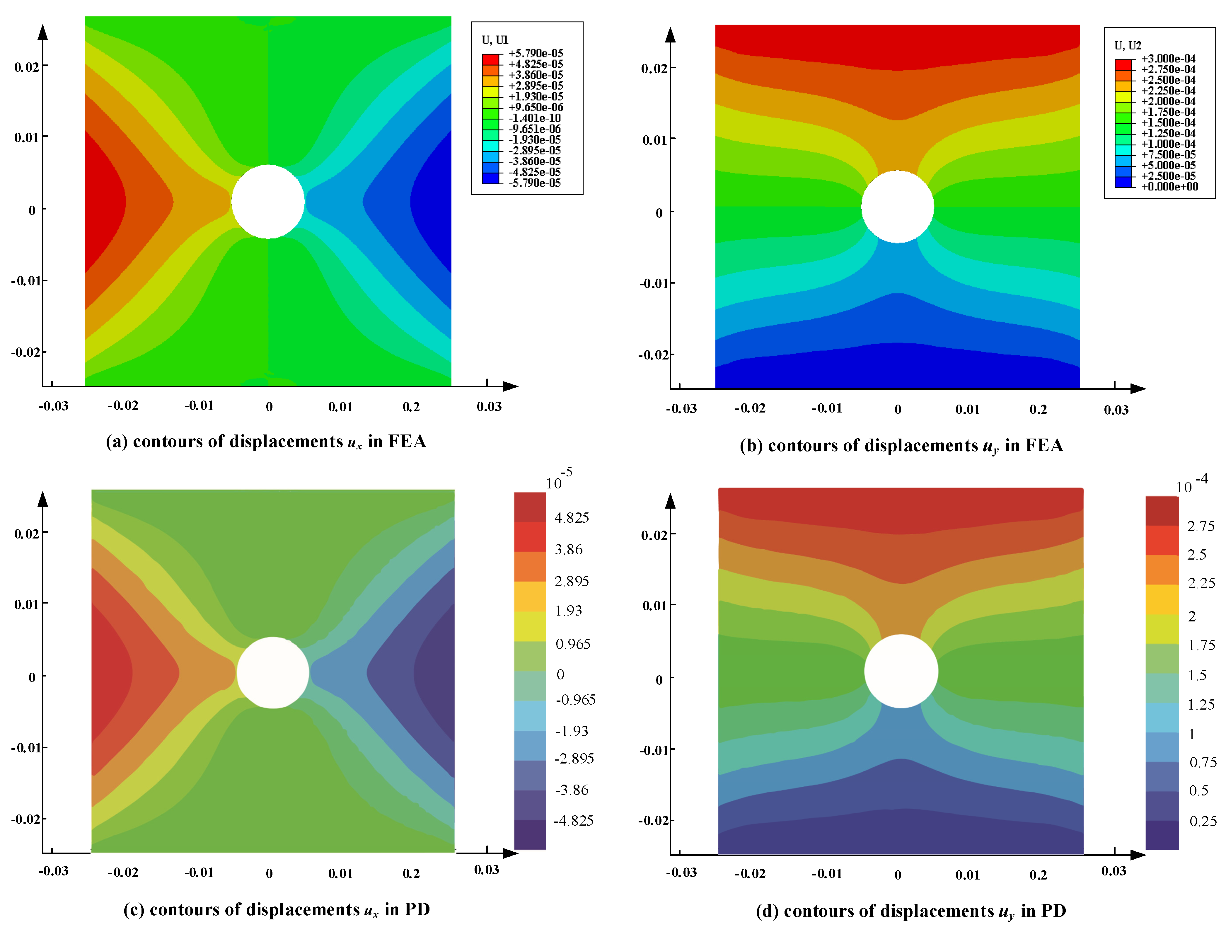
Except for the above local verification, the displacement cloud maps of $u_x$ and $u_y$, which can better reflect the overall deformation, are also compared, as shown in Figure 8 (e.g., $\delta =3\Delta x$). It is evident that the deformation distribution obtained by the PD model is well in line with the FEM results. There is little difference in displacement, $u_y$, between results from the two methods (as depicted in Figure 8b,d). Moreover, the maximum relative error of displacement, $u_x$, is no more than 0.8% (as revealed in Figure 8a,c). It indicates that the PD model established has the characteristics of rationality and accuracy.

5.2. Analysis of Quantitative Accuracy

The effect of numerical modulus coupling with different influence functions on deformation analysis is explored in this subsection. A cantilever beam with dimensions of 0.8 m × 0.2 m is shown in Figure 9. A concentrated force of F = 10 kN is applied at the midpoint of the right end. Material properties and the PD model parameters are illustrated in

Table 5. Material properties and PD model parameters.

E (GPa)	G (GPa)	v	$\mathit{\rho }$ (kg/m3)	$\mathsf{\Delta }\mathit{x}$ (m)	Influence Function
24.8	9.2	1/3	2400	0.02	$g_1-g_8$

. On the basis of the elasticity theory, the theoretical solution for the deflection curve in the central axis is given by Equation (25).

$$u_y=-\frac{F{(L-x)}^3}{6EI}+\frac{F{L}^2(L-x)}{2EI}-\frac{F{L}^3}{3EI}-\frac{3Fx}{2GA}$$

(25)

where L and I are the length and the inertia moment of the beam, respectively.

Regarding the selection of horizon radius, a series of numerical experiments are conducted. The computer configuration used in this work is Inter(R) Core(TM) i7-7700 CPU @ 3.60 GHz. Figure 10 illustrates the computing time for each influence function under different horizon radii. The computation cost increases with the increase in the horizon radius, which is the same as the conclusion in Section 5.1. As for accuracy, under different horizon radii, the relative error between the PD model using different influence functions and the theoretical results is less than 10%, which is within the acceptable range. Overall, the relative error is minimal when $\delta =3\Delta x$. Thus, $\delta =3\Delta x$ is adopted in the subsequent content.

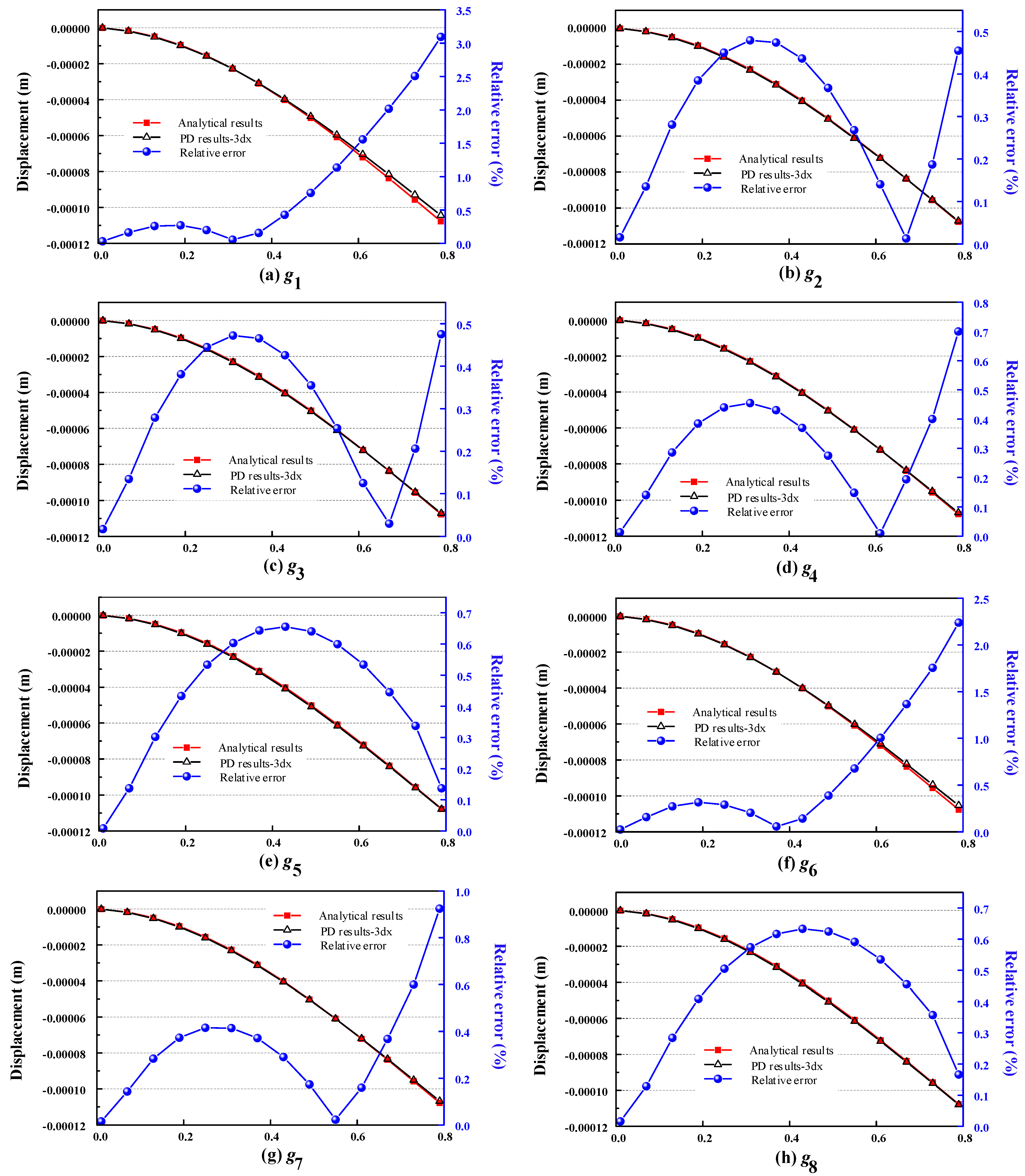
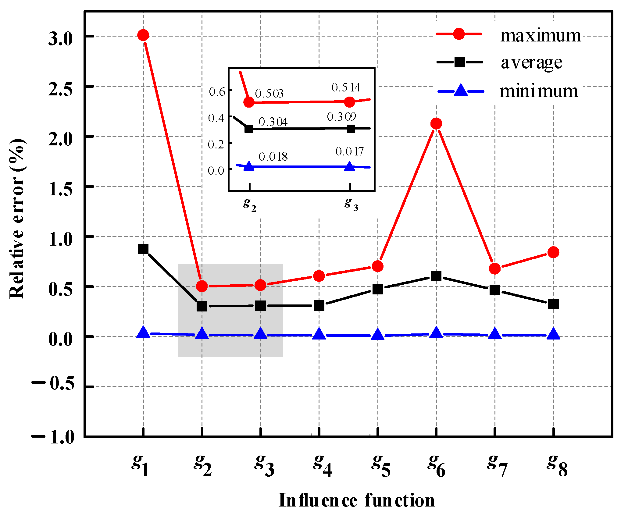
Figure 11 depicts a comparison between numerical solutions and analytical solutions for different influence functions. Moreover, the eigenvalues of relative error are listed in Figure 12.

The influence functions can ensure the model with good precision. Regardless of the type of influence function used, the relative error can be reduced to varying degrees compared with the traditional model (PD-g₁). Nevertheless, all relative error eigenvalues are within acceptable limits and the maximum relative errors are all less than 3.5% under different influence functions. In particular, the influence functions $g_2$ and $g_3$ make the greatest contribution to improving calculation accuracy.

On the whole, the exponential function $g_2=e^{-\xi /\delta }$ has the best computational accuracy, which can be seen from the local magnification in Figure 12.

5.3. Qualitative Failure Analysis

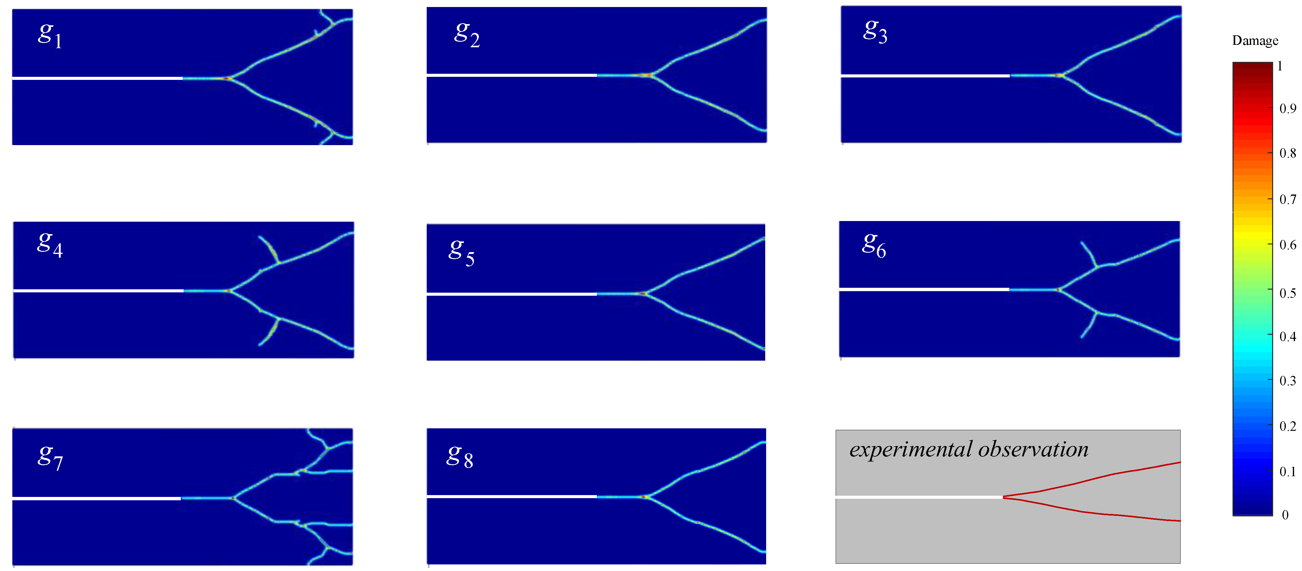
PD theory can correctly analyze the crack propagation in quasi-brittle materials [37,41], and the crack initiation and propagation are sensitive to the influence function [33]. In this section, a simulation on a typical mode-I fracture is carried out to investigate the impact of different influence functions on the crack extension morphology. The results are compared with experimental observation [42]. Then, the more effective influence function is selected by considering the simulation accuracy and stability.

The geometrical condition of a precast notched brittle plate is revealed in Figure 13. The purpose of the precast notch is to clearly track the crack path. The upper and lower edges of the plate are subjected to a tensile stress load of 12 MPa. Material properties and PD model parameters are illustrated in

Table 6. Material properties and PD model parameters.

E (GPa)	v	$\mathit{\rho }$ (kg/m3)	$\mathsf{\Delta }\mathit{x}$ (m)	$\mathit{\delta }$ (m)	$\mathsf{\Delta }\mathit{t}$ (m)	${\mathit{s}}_0$	Influence Function
65	1/3	2235	$0.25\times {10}^{-3}$	$3\Delta x$	$25ns$	$2.0934\times {10}^{-3}$	$g_1-g_8$

.

To assess the stability of crack growth, it is essential to determine if the crack growth velocity is within the theoretical limit of steady-state type-I fracture. The theoretical limit value is the Rayleigh wave speed, as calculated in Equation (26) [43]. The crack-tip is confirmed by tracing the rightmost point of $D(x,t)=0.35$. The crack propagation velocity is determined in Equation (27).

$$V_R=\frac{0.862+1.14v}{1+v}{V}_s$$

(26)

where $V_s$ is the transverse wave velocity, denoted as $V_s=\sqrt{\frac{u}{\rho }}=\sqrt{\frac{E}{2\rho (1+v)}}$

$$v_{crack}=‖\frac{x_c-x_{c-1}}{t_c-t_{c-1}}‖$$

(27)

in which $x_c$ and $x_{c-1}$ denote the crack-tip positions at time $t_c$ and $t_{c-1}$.

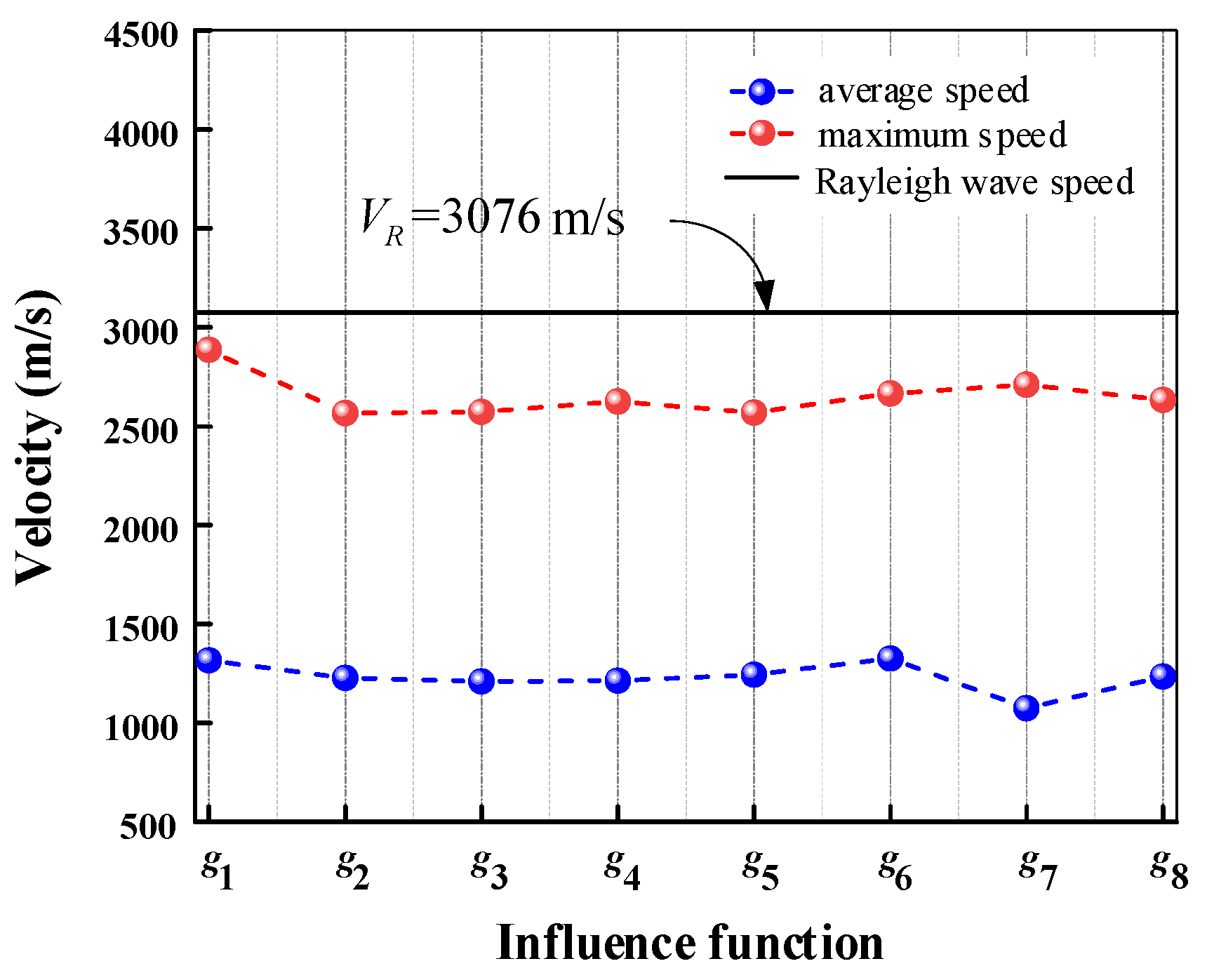
Figure 14 presents the average and maximum crack propagation velocities under various influence functions. These eigenvalues are all less than $V_R=3076 \mathrm{m}/\mathrm{s}$, which satisfies the stable propagation condition. This indicates that the cracks exhibit steady-state expansion under different influence functions.

It is predictable that the damage will initially appear at the precast notch, where the maximum stress is located. As seen in Figure 15, the crack morphology is affected by the type of influence function, which is consistent with the findings of previous study [38]. However, the initial damage position and the main crack propagation paths observed in the simulation are similar to these discovered in experiment, that is, linear propagation first, followed by branching propagation, which has proved the ability to simulate material failure. In particular, the crack growth patterns obtained by influence functions $g_2$, $g_3$, $g_5$ and $g_8$ appear remarkably well in line with the experimental phenomenon.

Combined with the research results in Section 5.2, the influence function $g_2$ is the more effective influence function by a comprehensive trade-off between simulation accuracy and stability. To further illustrate the rationality of $g_2$, Figure 16 depicts the change of PD force density and the crack evolution process.

The PD force density is mainly concentrated at the pre-notch tip, where the damage initially occurs. As the PD force density increases near the tip, the accumulated wave promotes horizontal crack propagation, similar to the typical mode-I crack. At 850 steps, the horizontal propagation distance is 0.017 m. Subsequently, the main crack branches spontaneously and symmetrically, and the maximum PD force density appeared at the branches. Moreover, the greater PD force density could also be observed between the branching cracks. At 1350 steps, the horizontal propagation distance of the crack is 0.031 m. At 2000 steps, the crack reaches the free boundary with the horizontal crack propagation distance of 0.05 m, just as observed in the experimental studies, and a part of PD force density has a wavelet diffusion. The correspondence between the PD force density and crack propagation is in accordance with the physical law.

6. Conclusions

In this work, the numerical micromodulus is derived for the plane stress problem within the frame of BBPD. Then, several influence functions representing the spatial intensity distribution of nonlocal force are introduced into the numerical micromodulus. Furthermore, a load increment algorithm based on fictitious density is developed for quasi-static analysis and the iteration algorithm is discussed. Several typical applications are investigated to determine the more effective influence function according to accuracy of deformation and fracture morphology for brittle materials. The main conclusions can be drawn as follows:

According to the concept of peridynamic stress, numerical micromoduli under commonly used horizon radii are derived for the plane stress problem, which provides a valuable insight for the application of bond-based peridynamics. Nevertheless, further research, such as in the nonuniform deformation condition, is required in future.

The introduction of the influence function can enhance the analysis precision on deformation and failure, which is beneficial to the generalization and application of numerical micromoduli. Through a comprehensive trade-off between simulation accuracy and stability, the numerical micromodulus coupled with the exponential influence function proves to be a more effective option for brittle materials.

The load increment algorithm based on fictitious density proposed in this work is effective in analyzing quasi-static problems. Since the fictitious density and safety factor are included in the load increment qualification, the premature failure due to excessive load increments can be avoided.

References

1. Silling, S.A. Reformulation of Elasticity Theory for Discontinuities and Long-Range Forces. J. Mech. Phys. Solids 2000, 48, 175–209. [Google Scholar] [CrossRef]
2. Chen, Z.; Chu, X.; Duan, Q. A Micromorphic Peridynamic Model and the Fracture Simulations of Quasi-Brittle Material. Eng. Fract. Mech. 2022, 271, 108631. [Google Scholar] [CrossRef]
3. Silling, S.A.; Weckner, O.; Askari, E.; Bobaru, F. Crack Nucleation in a Peridynamic Solid. Int. J. Fract. 2010, 162, 219–227. [Google Scholar] [CrossRef]
4. Basoglu, M.F.; Zerin, Z.; Kefal, A.; Oterkus, E. A Computational Model of Peridynamic Theory for Deflecting Behavior of Crack Propagation with Micro-Cracks. Comput. Mater. Sci. 2019, 162, 33–46. [Google Scholar] [CrossRef]
5. Deng, X.; Wang, B. Peridynamic Modeling of Dynamic Damage of Polymer Bonded Explosive. Comput. Mater. Sci. 2020, 173, 109405. [Google Scholar] [CrossRef]
6. Breitenfeld, M.S.; Geubelle, P.H.; Weckner, O.; Silling, S.A. Non-Ordinary State-Based Peridynamic Analysis of Stationary Crack Problems. Comput. Methods Appl. Mech. Eng. 2014, 272, 233–250. [Google Scholar] [CrossRef]
7. Silling, S.A. Dynamic Fracture Modeling with a Meshfree Peridynamic Code. In Computational Fluid and Solid Mechanics 2003, Proceedings of the Second MIT Conference on Compurational Fluid and Solid Mechanics, Cambridge, MA, USA, 17–20 June 2003; Bathe, K.J., Ed.; Elsevier Science Ltd.: Oxford, UK, 2003; pp. 641–644. ISBN 978-0-08-044046-0. [Google Scholar]
8. Weckner, O.; Abeyaratne, R. The Effect of Long-Range Forces on the Dynamics of a Bar. J. Mech. Phys. Solids 2005, 53, 705–728. [Google Scholar] [CrossRef]
9. Zhang, Y.; Deng, H.; Deng, J.; Liu, C.; Yu, S. Peridynamic Simulation of Crack Propagation of Non-Homogeneous Brittle Rock-like Materials. Theor. Appl. Fract. Mech. 2020, 106, 102438. [Google Scholar] [CrossRef]
10. Zhou, L.M.; Zhu, S.; Zhu, Z.D.; Xie, X.H. Simulations of Fractures of Heterogeneous Orthotropic Fiber-Reinforced Concrete with Pre-Existing Flaws Using an Improved Peridynamic Model. Materials 2022, 15, 3977. [Google Scholar] [CrossRef]
11. Rivera, J.; Berjikian, J.; Ravinder, R.; Kodamana, H.; Das, S.; Bhatnagar, N.; Bauchy, M.; Krishnan, N.M.A. Glass Fracture Upon Ballistic Impact: New Insights from Peridynamics Simulations. Front. Mater. 2019, 6, 239. [Google Scholar] [CrossRef]
12. Shi, Z.; Yue, J.; Xu, L.; Wang, X. Peridynamics for Fracture Analysis of Reflective Cracks in Semi-Rigid Base Asphalt Pavement. Appl. Sci. 2022, 12, 3486. [Google Scholar] [CrossRef]
13. Han, J.; Chen, W. An Ordinary State-Based Peridynamic Model for Fatigue Cracking of Ferrite and Pearlite Wheel Material. Appl. Sci. 2020, 10, 4325. [Google Scholar] [CrossRef]
14. Jiang, X.-W.; Guo, S.; Li, H.; Wang, H. Peridynamic Modeling of Mode-I Delamination Growth in Double Cantilever Composite Beam Test: A Two-Dimensional Modeling Using Revised Energy-Based Failure Criteria. Appl. Sci. 2019, 9, 656. [Google Scholar] [CrossRef]
15. Guan, J.; Yan, X.; Guo, L. An Improved Bond-Based Peridynamic Model with Shear Bonds for Eliminating Rigid Body Rotation. Theor. Appl. Fract. Mech. 2022, 119, 103369. [Google Scholar] [CrossRef]
16. Huang, D.; Lu, G.; Wang, C.; Qiao, P. An Extended Peridynamic Approach for Deformation and Fracture Analysis. Eng. Fract. Mech. 2015, 141, 196–211. [Google Scholar] [CrossRef]
17. Ha, Y.D. An Extended Ghost Interlayer Model in Peridynamic Theory for High-Velocity Impact Fracture of Laminated Glass Structures. Comput. Math. Appl. 2020, 80, 744–761. [Google Scholar] [CrossRef]
18. Silling, S.A.; Bobaru, F. Peridynamic Modeling of Membranes and Fibers. Int. J. Non. Linear. Mech. 2005, 40, 395–409. [Google Scholar] [CrossRef]
19. Postek, E.; Sadowski, T.; Boniecki, M. Impact of Brittle Composites: Peridynamics Modelling. Mater. Today Proc. 2021, 45, 4268–4274. [Google Scholar] [CrossRef]
20. Jenabidehkordi, A.; Abadi, R.; Rabczuk, T. Computational Modeling of Meso-Scale Fracture in Polymer Matrix Composites Employing Peridynamics. Compos. Struct. 2020, 253, 112740. [Google Scholar] [CrossRef]
21. Shi, C.; Shi, Q.; Tong, Q.; Li, S. Peridynamics Modeling and Simulation of Meso-Scale Fracture in Recycled Coarse Aggregate (RCA) Concretes. Theor. Appl. Fract. Mech. 2021, 114, 102949. [Google Scholar] [CrossRef]
22. Huang, D.; Lu, G.; Qiao, P. An Improved Peridynamic Approach for Quasi-Static Elastic Deformation and Brittle Fracture Analysis. Int. J. Mech. Sci. 2015, 94–95, 111–122. [Google Scholar] [CrossRef]
23. Jo, G.; Ha, Y.D. Two-Grid Based Sequential Peridynamic Analysis Method for Quasi-Static Crack Propagation. Eng. Fract. Mech. 2022, 269, 108549. [Google Scholar] [CrossRef]
24. Silling, S.A.; Askari, E. A Meshfree Method Based on the Peridynamic Model of Solid Mechanics. Comput. Struct. 2005, 83, 1526–1535. [Google Scholar] [CrossRef]
25. Gu, X.; Zhang, Q.; Huang, D.; Yv, Y. Wave Dispersion Analysis and Simulation Method for Concrete SHPB Test in Peridynamics. Eng. Fract. Mech. 2016, 160, 124–137. [Google Scholar] [CrossRef]
26. Qin, H.-Y.; Huang, D.; Liu, Y.-M.; Zhang, Q. An Extended Peridynamic Approach for Analysis of Multiple Crack Growth. Gongcheng Lixue Eng. Mech. 2017, 34, 31–38. [Google Scholar] [CrossRef]
27. Das, S.; Hoffarth, C.; Ren, B.; Spencer, B.; Sant, G.; Rajan, S.D.; Neithalath, N. Simulating the Fracture of Notched Mortar Beams through Extended Finite-Element Method and Peridynamics. J. Eng. Mech. 2019, 145, 04019049. [Google Scholar] [CrossRef]
28. Torrence, C.E.; Trageser, J.E.; Jones, R.E.; Rimsza, J.M. Sensitivity of the Strength and Toughness of Concrete to the Properties of the Interfacial Transition Zone. Constr. Build. Mater. 2022, 336, 126875. [Google Scholar] [CrossRef]
29. Li, W.; Guo, L. A Mechanical-Diffusive Peridynamics Coupling Model for Meso-Scale Simulation of Chloride Penetration in Concrete under Loadings. Constr. Build. Mater. 2020, 241, 118021. [Google Scholar] [CrossRef]
30. Rao, F.; Zhang, Z.; Ye, G. Three-Dimensional Mesoscale Modeling of Foamed Cement Paste Using Peridynamics. Constr. Build. Mater. 2021, 310, 125230. [Google Scholar] [CrossRef]
31. Hou, D.; Zhang, W.; Ge, Z.; Wang, P.; Wang, X.; Zhang, H. Experimentally Validated Peridynamic Fracture Modelling of Mortar at the Meso-Scale. Constr. Build. Mater. 2021, 267, 120939. [Google Scholar] [CrossRef]
32. Liu, W.; Hong, J.-W. Discretized Peridynamics for Linear Elastic Solids. Comput. Mech. 2012, 50, 579–590. [Google Scholar] [CrossRef]
33. Li, S.; Jin, Y.; Lu, H.; Sun, P.; Huang, X.; Chen, Z. Wave Dispersion and Quantitative Accuracy Analysis of Bond-Based Peridynamic Models with Different Attenuation Functions. Comput. Mater. Sci. 2021, 197, 110667. [Google Scholar] [CrossRef]
34. Li, X.; Gu, X.; Xia, X.; Madenci, E.; Chen, X.; Zhang, Q. Effect of Water-Cement Ratio and Size on Tensile Damage in Hardened Cement Paste: Insight from Peridynamic Simulations. Constr. Build. Mater. 2022, 356, 129256. [Google Scholar] [CrossRef]
35. Gerstle, W.; Sau, N.; Aguilera, E. Micropolar Peridynamic Modeling of Concrete Structures BT. In Proceedings of the 6th International Conference on Fracture Mechanics of Concrete and Concrete Structures, Catania, Italy, 17–22 June 2007; Taylor and Francis: Balkema, Slovakia, 2007; Volume 1. [Google Scholar]
36. Gerstle, W.H.; Sau, N.; Sakhavand, N. On Peridynamic Computational Simulation of Concrete Structures BT. In Proceedings of the ACI Fall 2009 Convention, New Orleans, LA, USA, 8–12 November 2009; American Concrete Institute: Farmington Hills, MI, USA, 2009; pp. 245–264. [Google Scholar]
37. Ha, Y.D.; Bobaru, F. Studies of Dynamic Crack Propagation and Crack Branching with Peridynamics. Int. J. Fract. 2010, 162, 229–244. [Google Scholar] [CrossRef]
38. Chen, Z.; Woody Ju, J.; Su, G.; Huang, X.; Li, S.; Zhai, L. Influence of Micro-Modulus Functions on Peridynamics Simulation of Crack Propagation and Branching in Brittle Materials. Eng. Fract. Mech. 2019, 216, 106498. [Google Scholar] [CrossRef]
39. Kilic, B.; Madenci, E. Structural Stability and Failure Analysis Using Peridynamic Theory. Int. J. Non. Linear. Mech. 2009, 44, 845–854. [Google Scholar] [CrossRef]
40. Kilic, B.; Madenci, E. An Adaptive Dynamic Relaxation Method for Quasi-Static Simulations Using the Peridynamic Theory. Theor. Appl. Fract. Mech. 2010, 53, 194–204. [Google Scholar] [CrossRef]
41. Ha, Y.D.; Bobaru, F. Characteristics of Dynamic Brittle Fracture Captured with Peridynamics. Eng. Fract. Mech. 2011, 78, 1156–1168. [Google Scholar] [CrossRef]
42. Ramulu, M.; Kobayashi, A.S. Mechanics of Crack Curving and Branching—A Dynamic Fracture Analysis. Int. J. Fract. 1985, 27, 187–201. [Google Scholar] [CrossRef]
43. Zhou, X.; Wang, Y.; Qian, Q. Numerical Simulation of Crack Curving and Branching in Brittle Materials under Dynamic Loads Using the Extended Non-Ordinary State-Based Peridynamics. Eur. J. Mech. A Solids 2016, 60, 277–299. [Google Scholar] [CrossRef]
Figure 1. Flowchart for this paper.
Applsci 13 05959 g001
Figure 2. Diagram of the BBPD.
Applsci 13 05959 g002
Figure 3. Bonds acting at the cross-section A i of point X i (δ = 2Δx).
Applsci 13 05959 g003
Figure 4. Bonds acting on the cross-section Ai ( δ = 2 Δ x ).
Applsci 13 05959 g004
Figure 5. Flowchart of the numerical implementation procedure.
Applsci 13 05959 g005
Figure 6. Scheme of the plate.
Applsci 13 05959 g006
Figure 7. Results along the x-axis and y-axis.
Applsci 13 05959 g007
Figure 8. Displacement contours (unit: m).
Applsci 13 05959 g008
Figure 9. Diagram of cantilever beam.
Applsci 13 05959 g009
Figure 10. Computation time of influence functions at different horizon radii.
Applsci 13 05959 g010
Figure 11. Displacements (red line and black line) and relative error (blue line) of the central axis for different influence functions ( δ = 3 Δ x , influence function symbol g i ,   i = 1 , 2 , 3 8  ).
Applsci 13 05959 g011
Figure 12. Eigenvalues of relative error.
Applsci 13 05959 g012
Figure 13. Schematic diagram of the plate.
Applsci 13 05959 g013
Figure 14. Crack propagation velocity eigenvalues under various influence functions.
Applsci 13 05959 g014
Figure 15. Crack propagation path under different influence functions and the redrawn experimental observation from [42].
Applsci 13 05959 g015
Figure 16. PD force density and crack evolution process using PD model g 2 .
Applsci 13 05959 g016